Advanced Model Predictive Control Part 10 doc

Predictive Control for Active Model and its Applications on Unmanned Helicopters

259
To verify the accuracy of the estimate of the model error, described in Fig.3, the following
experiment is designed:
1.
Actuate the longitudinal control loop to keep the speed more than 5 meter per second;
2.
Get the lateral model error value and boundaries through ASMF, and add them to the
hovering model we built above;
3.
Compare the model output before and after compensation for model error.
This process of experiment can be described by Fig.4, and the results are shown in Fig.5.
Fig.5a shows that model output (red line) cannot describe the cruising dynamics due to the
model error when ‘mode-change’, similar with Fig.3b; however, after compensation, shown
in Fig.5b, the model output (red line) is very close with real cruising dynamics (blue line),
and the uncertain boundaries can include the changing lateral speed, which mean that the
proposed estimation method can obtain the model error and range accurately by ASMF
when mode-change.


Fig. 4. The experiment process for model-error estimate

0 1000 2000 3000 4000 5000 6000 7000
-2
0
2
4
6
8

10
Sampling Time
(a)
Velocity/m/s
Model Accuracy before Compensation
Real Data
Model Output
0 1000 2000 3000 4000 5000 6000 7000
-2
-1
0
1
2
3
4
5
6
Sampling Point
(b)
Velocty/m/s
Lateral Velocty after Compensation
Real Velocity
Model Output
Up-boundary
Down-boundary

Fig. 5. Model output before/after compensation: (a) before compensation; (b) after
compensation

Advanced Model Predictive Control

260
5.3 Flight experiment for the comparison of GPC SIPC and AMSIPC when sudden
mode-change
In Section 5.2, the model-error occurrence and the accuracy of the proposed method for
estimation are verified. So, the next is the performance of the proposed controller in real
flight. In this section, the performance of the modified GPC (Generalized Predictive Control,
designed in Section 4.1), SIPC (Stationary Increment Predictive Control, designed in Section
4.2) and AMSIPC (Active Modeling Based Stationary Increment Predictive Control,
designed in Section 4.3), are tested in sudden mode-change, and are compared with each
other on the ServoHeli-40 test-bed. To complete this mission, the following experimental
process is designed:
1.
Using large and step-like reference velocity, red line in Fig.6-8, input it to longitudinal
loop, lateral loop and vertical loop;
2.
Based on the same inputted reference velocity, using the 3 types of control method,
GPC, SIPC and AMSIPC to actuate the helicopter to change flight mode quickly;
3.
Record the data of position, velocity and reference speed for the 3 control loops, and
obtain reference position by integrating the reference speed;
4.
Compare errors of velocity and position tracking of GPC, SIPC and AMSIPC,
executively, in this sudden mode-change flight.
GPC, SIPC and AMSIPC are all tested in the same flight conditions, and the comparison
results are shown in Figs. 6-8. We use the identified parameters in Section 5.2 to build the
nominal model, based on the model structure in Appendix A, and parameters’ selection in
Appendix C for controllers
It can be seen that, when the helicopter increases its longitudinal velocity and changes flight
mode from hovering to cruising, GPC (brown line) has a steady velocity error and increasing

position error because of the model errors. SIPC (blue line) has a smaller velocity error because
it uses increment model to reject the influence of the changing operation point and dynamics’
slow change during the flight. The prediction is unbiased and obtains better tracking
performance, which is verified by Theorem. However, the increment model may enlarge the
model errors due to the uncertain parameters and sensor/process noises, resulting in the
oscillations in the constant velocity period (clearly seen in Fig.6&7) because the error of its
prediction is only unbiased, but not minimum variance. While for AMSIPC (green line),
because the model error, which makes the predictive process non-minimum variance, has


Fig. 6. Longitudinal tracking results: (a) velocity; (b) position error (<50s hovering, >50s
cruising)

Predictive Control for Active Model and its Applications on Unmanned Helicopters

261

Fig. 7. Lateral tracking results: (a) velocity; (b) position error (25s~80s cruising, others
hovering)

Fig. 8. Vertical tracking results: (a) velocity; (b) position error (<5s hovering; >5s cruising)
been online estimated by the ASMF and compensated by the strategy in section 4.3, the
proposed AMSIPC successfully reduces velocity oscillations and tracking errors together.
6. Conclusion
An active model based predictive control scheme was proposed in this paper to compensate
model error due to flight mode change and model uncertainties, and realize full flight
envelope control without multi-mode models and mode-dependent controls.
The ASMF was adopted as an active modeling technique to online estimate the error
between reference model and real dynamics. Experimental results have demonstrated that
the ASMF successfully estimated the model error even though it is both helicopter dynamics

and flight-state dependent.In order to overcome the aerodynamics time-delay, also with the
active estimation for optimal compensation, an active modeling based stationary increment
predictive controller was designed and analyzed.
The proposed control scheme was implemented on our developed ServoHeli-40 unmanned
helicopter. Experimental results have demonstrated clear improvements over the normal
GPC without active modeling enhancement when sudden mode-change happens.
It should be noted that, at present, we have only tested the control scheme with respect to
the flight mode change from hovering to cruising, and vice versa. Further mode change
conditions will be flight-tested in near future.

Advanced Model Predictive Control

262
7. Appendix
A. Helicopter dynamics
A helicopter in flight is free to simultaneously rotate and translate in six degrees of freedom.
Fig. A-1 shows the helicopter variables in a body-fixed frame with origin at the vehicle’s
center of gravity.


Fig. A-1. Helicopter with its body-fixed reference frame
Ref.[18] developed a semi-decoupled model for small-size helicopter, i.e.,
00
00 0
010 0 0
00
0101/ /
010 0 1/
ua
lon lat

ua
lon lat
lon
lat
fcf
lon lat
flonlat
XgX
uuXX
MM
qqMM
A
aaAA
ccCC



 





  

  

  



  



  



  

  


  






, i.e.,


33 32
0
lon lon lon lon lon
lon lon lon lon
XAXBu
yI XCX












(A-1)
00
00 0
010 0 0
00
0101/ /
010 0 1/
ua
lon lat
ua
lon lat
lon
lat
lat
fdf
lon lat
flonlat
vYgY
vYY
pL L

pLL
X
B
bbBB
dDD
d











  
 
  
 
  
 

  
 
 

  
 



  
 
  
 
  

 
  






, i.e.,


33 32
0
lat lat lat lat lat
lat lat lat lat
XAXBu
y
IXCX












(A-2)
0
000
ped col
wr
p
ed
yaw heave w r ped ped col
col
fb fb
rrfb
ZZ
wZZw
rX NNN rNN
rr
KK


 





  


  
  


  



  


  





, i.e.

Predictive Control for Active Model and its Applications on Unmanned Helicopters

263


22 21
0
yaw heave yaw heave yaw heave yaw heave yaw heave

y
aw heave
y
aw heave
y
aw heave
y
aw heave
XAXBu
yI XCX



  








(A-3)
where δu, δv, δw are longitudinal, lateral and vertical velocity, δp, δq, δr are roll, pitch and
yaw angle rates, δφ and δθ are the angles of roll and pitch, respectively, a and b are the first
harmonic flapping angle of main rotor, c and d are the first harmonic flapping angle of
stabilizer bar,
f
b
r


is the feedback control value of the angular rate gyro,
lat

is the lateral
control input,
lon

is the longitudinal control input,
p
ed

is the yawing control input, and
col

is the vertical control input. All the symbols except gravity acceleration g in
lon
A
,
lat
A
,
y
aw heave
A

,
lon
B ,
lat

B and
y
aw heave
B

are unknown parameters to be identified. Thus, all of the
states and control inputs in (A-1), (A-2) and (A-3) are physically meaningful and defined in
body-axis.
B. Proof for the predictive theorem
Proof:
Assume the real dynamics is described as:

1tdrtdrtkt
XAXBUW


 (B-1)
which is different from the reference model of Eq. (11). In Eq. (B-1),
t
X is system state,
dr
A
is
the system matrix,
dr
B is the control matrix,
t
U is control input,
t
W is process noise. The

one-step prediction, according to Eq. (B-1), can be obtained by Eq. (13-14),

|1
111
ˆ
tt t d t d t k
dr t dr t k t
dt dtk
XXAXBU
AX BU W
AX BU


 


 

(B-2)
And



11|
111
ˆ
{
()}
{( ) ( ) }
ttt

dr t dr t k t
dr t dr t k t d t d t k
dr d t dr d t k t
EX X
EA X BU W
AX BU W A X B U
EA A X B B U W


 



 

(B-3)
According to condition 1) and 2), prediction is bounded, then,
11|
ˆ
ttt
XX



and, when the system of Eq. (B-1) works around a working point in steady state, the mean
value of control inputs and states should be constant, so we can obtain:



11|

ˆ
(){}(){}{}
()0()000
ttt
dr d t dr d t k t
dr d dr d
EX X
A AEX B BEU EW
AA BB



   

(B-4)

Advanced Model Predictive Control

264
Eq. (B-4) indicates that the one step prediction of Eq. (B-2) is unbiased.
Assuming that prediction at time i-1 is unbiased, i.e

11|
ˆ
{}0
ti ti t
EX X
 

 (B-5)

for the prediction at time i, there is

|
111
1| 1| 1
1111
11| 2
1| 1
11|
ˆ
{}
{
ˆ
ˆ
()}
{
ˆ
()
ˆ
}
ˆ
{
ti tit
dr t i dr t i k t i
ti t d ti t d ti k
dr t i dr t i k t i t i
ti ti t ti
dtit dtik
dr t i d t i t
EX X

EA X B U W
XAXBU
EA X B U W X
XX W
AX BU
EA X A X

   
   

    
  
 
 




 
 

11
1
11
() }
(){}
(){ }{}
()0()000
dr d t i k t i
dr d t i

dr d t i k t i
dr d dr d
BBU W
AAEX
BBEU EW
AA BB
  

  

 
  
 

(B-6)
Therefore, the prediction at time i is also unbiased.
C. Parameters’ selection for estimate and control in flight experiment
1. For Modeling
The identification results for hovering dynamics are listed in Tab.D-1.

Longitudinal Loop Lateral Loop Vertical Loop
Para. Val. Para. Val. Para. Val.
Xu 0.2446 Yv -0.0577 Zw 1.666
Xa -4.962 Yb 9.812 Zr -3.784
Xlat -0.0686 Ylat -1.823 Zped 2.304
Xlon 0.0896 Ylon 2.191 Zcol -11.11
Mu -1.258 Lv 15.84 Yaw Loop
Ma 46.06 Lb 126.6 Para. Val.
Mlat -0.6269 Llat -4.875 Nw -0.027
Mlon 3.394 Llon 28.64 Nr -1.087

Ac 0.1628 Bd -1.654 Nrfb -1.845
Alat -0.0178 Blat 0.04732 Nped 1.845
Alon -0.2585 Blon -9.288 Ncol -0.972
Clat 2.238 Dlat -0.7798 Kr -0.040
Clon -4.144 Dlon -5.726 Krfb -2.174
tf 0.5026 ts 0.5054
Table D-1. The parameters of hovering model

Predictive Control for Active Model and its Applications on Unmanned Helicopters

265
2. For ASMF
13 13 13 13
13 13 13 13
0.01 0
00.1
I
Q
I






,
88
0.01RI



where
mm
I

is the m×m unit matrix and
0
mn

is the m×n zero matrix.
3.
For GPC
10p

,
40 40
2.32I



, 10k


4.
For SIPC
10p

,
44
2.32I




,
88
0.99I




80 80
WI

 , 10k

,
44
0.8I



5.
For AMSIPC
10p 
,
44
2.32I




,
88
0.99I




80 80
WI


, 10k

,
44
0.8I


 ,
13 13
HI



8. References
Tischler M.B., “Frequency-domain Identification of XV-15 Tilt-rotor Aircraft Dynamics in
Hovering Flight,” Journal of the American Helicopter Society, Vol. 30 (2), pp.38-48,
1985.
Tischler M. B. and Cauffman M. G., “Frequency-Response Method for Rotorcraft System
Identification: Flight Application to BO-I05 Coupled Rotor/Fuselage Dynamics,”

Journal of the American Helicopter Society, Vol. 37 (3), pp.3-17, 1992.
Fletcher J. W., “Identification of UH-60 Stability Derivative Models in Hover from Flight
Test Data,” Journal of the American Helicopter Society, Vol. 40 (1), pp.8-20, 1995.
Mettler B., Tischler M. B. and Kanade T., “System Identification of Small-Size Unmanned
Helicopter Dynamics,” American Helicopter Society 55th Annual Forum
Proceedings, Vol. 2, pp.1706-1717, Montreal, Quebec, Canada, May 25-27, 1999.
Gavrilets V., Metlter B. and Feron E., “Nonlinear Model for a Small-scale Acrobatic
Helicopter,” Proceedings of the American Institute of Aeronautics Guidance,
Navigation, and Control Conference, pp.8, Montreal, Quebec, Canada, August 6-9,
2001.
Massimiliano M. and Valerio S., “A Full Envelope Small Commercial Aircraft Flight Control
Design Using Multivariable Proportional-Integral Control,” IEEE Transactions on
Control Systems Technology, Vol. 16 (1), pp.169-176, January, 2008.
Voorsluijs M. and Mulder A., "Parameter-dependent robust control for a rotorcraft UAV,"
AIAA Guidance, Navigation, and Control Conference and Exhibit, pp.1-11, San
Francisco, California, USA, August 15-18, 2005.
Bijnens B., Chu Q.P. and Voorsluijs M., "Adaptive feedback linearization flight control for a
helicopter UAV," AIAA Guidance, Navigation, and Control Conference and
Exhibit, pp.1-10, San Francisco, California, USA, August 15-18, 2005.
Kahveci N.E., Ioannou P.A., Mirmirani M.D., “Adaptive LQ Control With Anti-Windup
Augmentation to Optimize UAV Performance in Autonomous Soaring

Advanced Model Predictive Control

266
Applications,” IEEE Transactions on Control Systems Technology, Vol. 16(4):
pp.691 – 707, 2008
MacKunis W., Wilcox Z.D., Kaiser M.K., Dixon W.E., “Global Adaptive Output Feedback
Tracking Control of an Unmanned Aerial Vehicle,” IEEE Transactions on Control
Systems Technology, Vol. 18(6): pp.1390-1397, 2010.

Cummings M.L., Mitchell P.J., “Predicting Controller Capacity in Supervisory Control of
Multiple UAVs Systems,” IEEE Transactions on Man and Cybernetics, Part A:
Systems and Humans, Vol. 38(2): pp.451-460, 2008.
Jiang X., Han Q.L., “On guaranteed cost fuzzy control for nonlinear systems with interval
time-varying delay,” Control Theory & Applications, IET, Vol. 1(6): pp.1700-1710,
2007.
Natori K., Oboe R., Ohnishi, K., “Stability Analysis and Practical Design Procedure of Time
Delayed Control Systems With Communication Disturbance Observer,” IEEE
Transactions on Industrial Informatics, Vol. 4(3): pp.185-197, 2008.
Haykin S. and De Freitas N., “Special Issue on Sequential State Estimation,” Proceedings of
the IEEE, Vol. 92(3), pp.423-574, 2004.
Lerro D. and Bar-Shalom Y. K., ” Tracking with Debiased Consistent Converted
Measurements vs. EKF,” IEEE Transactions on Aerosp. Electron.System, AES-29,
pp.1015-1022, 1993
．
Julier S. and Uhlmann J., “Unscented filtering and nonlinear estimation,” Proceedings of the
IEEE, Vol. 92(3), pp. 401-422, 2004.
Song Q., Jiang Z., and Han J. D., “UKF-Based Active Model and Adaptive Inverse Dynamics
Control for Mobile Robot,” IEEE International Conference on Robotics and
Automation, 2007.
Shamma J. S. and Tu K. Y., “Approximate set-valued observers for nonlinear systems,” IEEE
Transactions on Automatic Control, Vol. 42(5), pp.648–658, 1997.
Zhou B., Han J.D. and Liu G., “A UD factorization-based nonlinear adaptive set-
membership filter for ellipsoidal estimation,” International Journal of Robust and
Nonlinear Control, Vol 18 (16), pp.1513-1531, November 10, 2007.
Scholte E., Campbell M.E., “Robust Nonlinear Model Predictive Control With Partial State
Information,” Control Systems Technology, IEEE Transactions on, Vol. 16(4):
pp.636-651, 2008.
Ding B. C., Xi Y. G., “A Synthesis Approach of On-line Constrained Robust Model
Predictive Control.” Automatica. Vol. 40(1): pp. 163-167, 2004.

Crassidis J. L., “Robust Control of Nonlinear Systems Using Model-Error Control
Synthesis,” Journal of guidance, control and dynamics, Vol. 22 (4), pp.595-601, 1999.
Gregor K. and Igor S., “Tracking-error Model-based Predictive Control for Mobile Robots in
real time.” Robotics and Autonomous Systems. Vol. 55, No. 7, pp. 460 - 469, 2007.
Qi J.T., Song D.L., Dai. L., Han J.D., “The ServoHeli-20 Rotorcraft UAV Project,”
International Conference on Mechatronics and Machine Vision in Practice,
Auckland, New Zealand, pp.92-96, 2008.
Song D.L., Qi J.T., Dai. L., Han J.D. and Liu G., “Modeling a Small-size Unmanned
Helicopter Using Optimal Estimation in The Frequency Domain,” International
Conference on Mechatronics and Machine Vision in Practice, Auckland, New
Zealand, December 2-4, pp.97-102, 2008.
Song D.L., Qi J.T. and Han J.D., “Model Identification and Active Modeling Control for
Small-Size Unmanned Helicopters: Theory and Experiment,” AIAA Guidance
Navigation and Control, Toronto, Canada, AIAA-2010-7858, 2010.
13
Nonlinear Autoregressive with Exogenous
Inputs Based Model Predictive Control for Batch
Citronellyl Laurate Esterification Reactor
Siti Asyura Zulkeflee, Suhairi Abdul Sata and Norashid Aziz
School of Chemical Engineering, Engineering Campus,
Universiti Sains Malaysia, Seri Ampangan,
14300 Nibong Tebal, Seberang Perai Selatan, Penang,
Malaysia
1. Introduction
Esterification is a widely employed reaction in organic process industry. Organic esters are
most frequently used as plasticizers, solvents, perfumery, as flavor chemicals and also as
precursors in pharmaceutical products. One of the important ester is Citronellyl laurate, a
versatile component in flavors and fragrances, which are widely used in the food, beverage,
cosmetic and pharmaceutical industries. In industry, the most common ester productions are
carried out in batch reactors because this type of reactor is quite flexible and can be adapted to

accommodate small production volumes (Barbosa-Póvoa, 2007). The mode of operation for a
batch esterification reactor is similar to other batch reactor processes where there is no inflow
or outflow of reactants or products while the reaction is being carried out. In the batch
esterification system, there are various parameters affecting the ester rate of reaction such as
different catalysts, solvents, speed of agitation, catalyst loading, temperature, mole ratio,
molecular sieve and water activity (Yadav and Lathi, 2005). Control of this reactor is very
important in achieving high yields, rates and to reduce side products. Due to its simple
structure and easy implementation, 95% of control loops in chemical industries are still using
linear controllers such as the conventional Proportional, Integral & Derivative (PID)
controllers. However, linear controllers yield satisfactory performance only if the process is
operated close to a nominal steady-state or if the process is fairly linear (Liu & Macchietto,
1995). Conversely, batch processes are characterized by limited reaction duration and by non-
stationary operating conditions, then nonlinearities may have an important impact on the
control problem (Hua et al., 2004). Moreover, the control system must cope with the process
variables, as well as facing changing operation conditions, in the presence of unmeasured
disturbances. Due to these difficulties, studies of advanced control strategy have received great
interests during the past decade. Among the advanced control strategies available, the Model
Predictive Control (MPC) has proved to be a good control for batch reactor processes (Foss et
al., 1995; Dowd et al., 2001; Costa et al., 2002; Bouhenchir et al., 2006). MPC has influenced
process control practices since late 1970s. Eaton and Rawlings (1992) defined MPC as a control
scheme in which the control algorithm optimizes the manipulated variable profile over a finite
future time horizon in order to maximize an objective function subjected to plant models and

Advanced Model Predictive Control
268
constraints. Due to these features, these model based control algorithms can be extended to
include multivariable systems and can be formulated to handle process constraints explicitly.
Most of the improvements on MPC algorithms are based on the developmental reconstruction
of the MPC basic elements which include prediction model, objective function and
optimization algorithm. There are several comprehensive technical surveys of theories and

future exploration direction of MPC by Henson, 1998, Morari & Lee, 1999, Mayne et al., 2000
and Bequette, 2007. Early development of this kind of control strategy, the Linear Model
Predictive Control (LMPC) techniques such as Dynamic Matrix Control (DMC) (Gattu and
Zafiriou, 1992) have been successfully implemented on a large number of processes. One
limitation to the LMPC methods is that they are based on linear system theory and may not
perform well on highly nonlinear system. Because of this, a Nonlinear Model Predictive
Control (NMPC) which is an extension of the LMPC is very much needed.
NMPC is conceptually similar to its linear counterpart, except that nonlinear dynamic
models are used for process prediction and optimization. Even though NMPC has been
successfully implemented in a number of applications (Braun et al., 2002; M’sahli et al., 2002;
Ozkan et al., 2006; Nagy et al., 2007; Shafiee et al., 2008; Deshpande et al., 2009), there is no
common or standard controller for all processes. In other words, NMPC is a unique
controller which is meant only for the particular process under consideration. Among the
major issues in NMPC development are firstly, the development of a suitable model that can
represent the real process and secondly, the choice of the best optimization technique.
Recently a number of modeling techniques have gained prominence. In most systems, linear
models such as partial least squares (PLS), Auto Regressive with Exogenous inputs (ARX)
and Auto Regressive Moving Average with Exogenous inputs (ARMAX) only perform well
over a small region of operations. For these reasons, a lot of attention has been directed at
identifying nonlinear models such as neural networks, Volterra, Hammerstein, Wiener and
NARX model. Among of these models, the NARX model can be considered as an
outstanding choice to represent the batch esterification process since it is easier to check the
model parameters using the rank of information matrix, covariance matrices or evaluating
the model prediction error using a given final prediction error criterion. The NARX model
provides a powerful representation for time series analysis, modeling and prediction due to
its strength in accommodating the dynamic, complex and nonlinear nature of real time
series applications (Harris & Yu, 2007; Mu et al., 2005). Therefore, in this work, a NARX
model has been developed and embedded in the NMPC with suitable and efficient
optimization algorithm and thus currently, this model is known as NARX-MPC.
Citronellyl laurate is synthesized from DL-citronellol and Lauric acid using immobilized

Candida Rugosa lipase (Serri et. al., 2006). This process has been chosen mainly because it is a
very common and important process in the industry but it has yet to embrace the advanced
control system such as the MPC in their plant operation. According to Petersson et al. (2005),
temperature has a strong influence on the enzymatic esterification process. The temperature
should preferably be above the melting points of the substrates and the product, but not too
high, as the enzyme’s activity and stability decreases at elevated temperatures. Therefore,
temperature control is important in the esterification process in order to achieve maximum
ester production. In this work, the reactor’s temperature is controlled by manipulating the
flowrate of cooling water into the reactor jacket. The performances of the NARX-MPC were
evaluated based on its set-point tracking, set-point change and load change. Furthermore,
the robustness of the NARX-MPC is studied by using four tests i.e. increasing heat transfer
coefficient, increasing heat of reaction, decreasing inhibition activation energy and a
Nonlinear Autoregressive with Exogenous Inputs
Based ModelPredictive Control for Batch Citronellyl Laurate Esterification Reactor
269
simultaneous change of all the mentioned parameters. Finally, the performance of NARX-
MPC is compared with a PID controller that is tuned using internal model control technique
(IMC-PID).
2. Batch esterification reactor
The synthesis of Citronellyl laurate involved an exothermic process where Citronellol
reacted with Lauric acid to produce Citronellyl Laurate and water.


Fig. 1. Schematic represent esterification of Citronellyl laurate
The esterification process took place in a batch reactor where the immobilized lipase catalyst
was mixed freely in the reactor. A layout of the batch esterification reactor with associated
heating and cooling configurations is shown in Fig.2.


Fig. 2. Schematic diagram of the batch esterification reactor.

Typical operating conditions were 310K and 1 bar. The reactor temperature was controlled
by manipulating the water flowrate within the jacket. The reactor’s temperature should not
exceed the maximal temperature of 320K, due to the temperature sensitivity of the catalysts
(Yadav & Lathi, 2004; Serri et. al., 2006; Zulkeflee & Aziz, 2007). The reactor’s temperature
control can be achieved by treating the limitation of the jacket’s flowrate, Fj, which can be
viewed as a state of the process and as the constraint control problem. The control strategy
proposed in this paper was designed to meet the specifications of the laboratory scale batch
CH
2
OH
+ C
12
H
24
O
2
Catalyst
CH2OOC
12
H
23
+ H
2
O
LAURIC ACID
CITRONELLYL
WATER
CITRONELLOL
PI
F

j
, T
jin
C
i
, T
r
T
jout
T
hot
T
cold


Advanced Model Predictive Control
270
reactor at the Control Laboratory of School of Chemical Engineering, University Sains
Malaysia, which has a maximum of 0.2 L/min limitation on the jacket’s flowrate. Therefore,
the constraint of the jacket’s flowrate will be denoted as F
jmax
= 0.2 L/min.
The fundamental equations of the mass and energy balances of the process are needed to
generate data for empirical model identification. The equations are valid for all ∈
[
0,∞
]
.
The reaction rate and kinetics are given by (Yadav & Lathi, 2004; Serri et. al., 2006; Zulkeflee
& Aziz, 2007):




=
[


]





























+
[


]
1+


[


]
 (1)




=
[


]














+
[


]
1+


[


]
+







[


]
+


[


]


[


]
(2)




=−
[


]





























+
[

]

1+


[


]
 (3)




=−
[


]














+
[


]
1+


[


]
+






[


]
+


[


]



[


]
(4)


=




/

(5)


=




/

(6)


=





/

(7)
where 

,

,

and 

are concentrations (mol/L) of Lauric acid, Citronellol, Citronellyl
laurate and water respectively; r
max
(mol l
-1
min
-1
g
-1
of enzyme) is the maximum rate of
reaction,

K
Ac
(mol l

-1
g
-1
of enzyme), K
Al
(mol l
-1
g
-1
of enzyme) and K
i
(mol l
-1
g
-1
of enzyme)
are the Michealis constant for Lauric acid, Citronellol and inhibition respectively; 

,


and 

are the pre-exponential factors (L mol/s) for inhibition, Lauric acid and Citronellol
respectively; 

,

and 


are the activation energy (J mol/K) for inhibition, acid lauric
and Citronellol respectively; R is the gas constant (J/mol K).
The reactor can be described by the following thermal balances (Aziz et al., 2000):




=∆



+


[

(

















)]
(8)




=
(













)







(9)


=

−

 (10)
where T
r
(K) , T
j
(K) and T
jin
is reactor, jacket and inlet jacket temperature respectively; ∆


(kJ/mol) is heat of reaction; V(l) and V
j
(l) is the volume of the reactor and jacket
respectively;

,

,

and 

are specific heats (J/mol K) of Lauric acid, Citronellol,

Citronellyl laurate and water respectively; 

is the water density (g/L) in the jacket;

is
Nonlinear Autoregressive with Exogenous Inputs
Based ModelPredictive Control for Batch Citronellyl Laurate Esterification Reactor
271
the flowrate of the jacket (L/min); 

(kW) is the heat transfer through the jacket wall; A and
U are the heat exchange area (m
2
) and the heat exchange coefficient (W/m
2
/K) respectively.
Eq. 1 - Eq. 10 were simulated using a 4
th
/5
th
order of the Runge Kutta method in MATLAB®
environment. The model of the batch esterification process was derived under the
assumption that the process is perfectly mixed where the concentrations of [], [], [],
[] and temperature of the fluid in the tank is uniform. Table 1 shows all the value of the
parameters for the batch esterification process under consideration. The validations of
corresponding dynamic models have been reported in Zulkeflee & Aziz (2007).

Parameters Units Values Parameters Units Values
A
Ac

A
Al
A
i
E
Ac
E
Al
E
i
T
ji

Cp
Ac
Cp
Al
Cp
Es
L mol/s
L mol/s
L mol/s
J mol/K
J mol/K
J mol/K
K
J/mol K
J/mol K
J/mol K
18.20871

24.04675
0.319947
-105.405
-66.093
-249.944
294
420.53
235.27
617.79
Cp
w
V
V
j



ΔH
rxn
α
β
U
A
R
J/mol K
L

L
J/m
3

kJ
-
-
J/s m
2
K
m
2

J/mol K
75.40
1.5
0.8
11.648
16.73
1
1
2.857
0.077
8.314
Table 1. Operating Conditions and Calculated Parameters
3. NARX model
The Nonlinear Autoregressive with Exogenous inputs (NARX) model is characterized by
the non-linear relations between the past inputs, past outputs and the predicted process
output and can be delineated by the high order difference equation, as follows:

(

)
=

(
−1
)
,…−

,
(
−1
)
…
(
−

)
+() (11)
where 
(

)
and () represents the input and output of the model at time  in which the
current output ()∈ℜ depends entirely on the current input 
(

)
∈ℜ. Here 

and 

are
the input and output orders of the dynamical model which are 


≥0, 

≥1. The function
 is a nonlinear function. 

=[
(
−1
)
…−


(
−1
)
…(−
)
]

denotes the system
input vector with a known dimension =

+

. Since the function  is unknown, it is
approximated by the regression model of the form:


(


)
=
(

)
.(−



)+
(

)
.(−



)+
(
,
)
.
(
−
)







.
(
−
)
+
(
,
)
.
(
−
)






.
(
−
)
+
(
,
)
.
(

−
)






.
(
−
)
+()
(12)

Advanced Model Predictive Control
272
where 
(

)
and 
(
,
)
are the coefficients of linear and nonlinear for originating exogenous
terms; 
(

)


(
,
)
are the coefficients of the linear and nonlinear autoregressive
terms; (,) are the coefficients of the nonlinear cross terms. Eq. 12 can be written in matrix
form:


()

(
+1
)
⋮
(+

)
=.

+.

+.[]

+.[]

+.[]

(13)
where

=[
(
0
)

(
1
)
…
(


)
]

(14)

=[
(
1
)

(
2
)
…

]

(15)

=[
(
0,0
)

(
0,1
)
…
(
0,

)

(
1,1
)
…
(


,

)
]

(16)

=[

(
1,1
)

(
1,2
)
…1,


(
2,2
)
…

,

]

(17)

=[
(
0,1
)

(
0,2
)
…0,



(
1,1
)
…

,

]

(18)

=[
(

)

(
−1
)
…
(


)
] (19)

=[
(

−1
)

(
−2
)
…

] (20)

=[
(

)
.
(

)

(

)
.
(
−1
)
…
(

)

.
(
−

)

(
−1
)
.
(
−1
)
…
(
−

)
.
(
−

)
] (21)

=
(
−1
)
.

(
−1
)

(
−1
)
.
(
−2
)
…
(
−1
)
.−


(
−2
)
.
(
−2
)
…−


.−


 (22)

=
(

)
.
(
−1
)
.
(
−2
)

(

)
.−


(
−1
)
.
(
−1
)

(

−

)
.−

 (23)
The Eq. 13 can alternatively be expressed as:

(

)
=[









]














(24)
Nonlinear Autoregressive with Exogenous Inputs
Based ModelPredictive Control for Batch Citronellyl Laurate Esterification Reactor
273
and can be simplified as:


=

.
̅
(25)
where


=() (26)



=[










] (27)


̅
=[]

(28)

Finally, the solution of the above identification problem is represented by

̅
=

\

(29)
The procedures for a NARX model identification is shown in Fig. 3. This model
identification process includes:





Fig. 3. NARX model identification procedure
Identification Pretesting
• Nonlinear study

• Interaction stud
y
Selection of input si
g
nals
Selection of model order for NARX model
Model validatio
n
Done
Is the model
ade
q
uate?
Design new test
data
Yes
No

Advanced Model Predictive Control
274
• Identification pre-testing: This study is very important in order to choose the important
controlled, manipulated and disturbance variables. A preliminary study of the response
plots can also gives an idea of the response time and the process gain.
• Selection of input signal: The study of input range has to be done, to calculate the
maximal possible values of all the input signals so that both inputs and outputs will be
within the desired operating conditions range. The selection of input signal would
allow the incorporation of additional objectives and constraints, i.e. minimum or
maximum input event separations which are desirable for the input signals and the
resulting process behavior.
• Selection of model order: The important step in estimating NARX models is to choose

the model order. The model performance was evaluated by the Means Squared Error
(MSE) and Sum Squared Error (SSE).
• Model validation: Finally, the model was validated with two sets of validation data
which were unseen independent data sets that are not used in NARX model parameter
estimation.
The details of the identification of NARX model for the batch esterification can be found at
Zulkeflee & Aziz (2008).
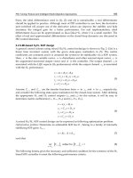
4. MPC algorithm
The conceptual structure of MPC is depicted in Fig. 4. The conception of MPC is to obtain the
current control action by solving, at each sampling instant, a finite horizon open-loop optimal
control problem, using the current state of the plant as the initial state. The desired objective
function is minimized within the optimization method and related to an error function based
on the differences between the desired and actual output responses. The first optimal input
was actually applied to the plant at time t and the remaining optimal inputs were discarded.
Meanwhile, at time t+1, a new measurement of optimal control problem was resolved and the
receding horizon mechanism provided the controller with the desired feedback mechanism
(Morari & Lee, 1999; Qin & Badgwell, 2003; Allgower, Findeisen & Nagy, 2004).






Fig. 4. Basic structure of Model Predictive Control
A formulation of the MPC on-line optimization can be as follows:

min

[


|

]
,…[|]

(
(

)
,
(

)
) (30)
OPTIMIZER PLANT
Output
setpoint
y
sp
(t)
Input u(t)
Output y(t)
Measurements
Nonlinear Autoregressive with Exogenous Inputs
Based ModelPredictive Control for Batch Citronellyl Laurate Esterification Reactor
275
min

[


|

]
,…[|]

∑


(
[
+
|

]
−

)

+
∑


∆[+|]





(31)

Where P and M is the length of the process output prediction and manipulated process
input horizons respectively with P ≤ M. [+|]
,…
is the set of future process input
values. The vector 

is the weight vector .
The above on-line optimization problem could also include certain constraints. There can be
bounds on the input and output variables:


≥[+|]≥

(32)

∆

≥∆[+|]≥−∆

(33)



≥[+|]≥

(34)

It is clear that the above problem formulation necessitates the prediction of future outputs

[+|]

In this NARX model, for k step ahead:
The error e(t):


[

|

]
=
(

)
−
(

)
.(−



)−
(

)
.(−




)−
(
,
)
.
(
−
)






.
(
−
)
−
(
,
)
.
(
−
)







.
(
−
)
−
(
,
)
.
(
−
)






.
(
−
)

(35)

The prediction of future outputs:



(
+
)
=
(

)
.(−



+)+
(

)
.(−



+)
+
(
,
)
.
(
−+
)







.
(
−+
)
+
(
,
)
.
(
−+
)






.
(
−+
)
+
(
,
)

.
(
−+
)






.
(
−+
)
+
(
+
)

(36)

Substitution of Eq. 35 and Eq. 36 into Eq 31 yields:

Advanced Model Predictive Control
276
min

[

|


]
,…[|]




(

)
.(−



++
(

)
.(−



+


+
(
,
)
.

(
−+
)






.
(
−+
)
+
(
,
)
.
(
−+
)






.
(
−+

)
+
(
,
)
.
(
−+
)






.
(
−+
)
+
(

)
−
(

)
.(−




)
−
(

)
.(−



)−
(
,
)
.
(
−
)






.
(
−
)
−
(

,
)
.
(
−
)






.
(
−
)
−
(
,
)
.
(
−
)







.
(
−
)
)
−

)

+

∆[+|]




(37)

Where



(

)
=[

(
+1
)



(
+2
)
….

(
+
)
]

(38)

∆
(

)
=[∆
[

|

]
∆
[
+1
|

]

…∆
[
+−1
|

]
]

(39)

The above optimization problem is a nonlinear programming (NLP) which can be solved at
each time t. Even though the input trajectory was calculated until M-1 sampling times into
the future, only the first computed move was implemented for one sampling interval and
the above optimization was repeated at the next sampling time. The structure of the
proposed NARX-MPC is shown in Fig. 5.
In this work, the optimization problem was solved using constrained nonlinear optimization
programming (fmincon) function in the MATLAB. A lower flowrate limit of 0 L/min and an
upper limit of 0.2 L/min and a lower temperature limit of 300K and upper limit of 320K
were chosen for the input and output variables respectively. In order to evaluate the
performance of NARX-MPC controller, the NARX-MPC has been used to track the
temperature set-point at 310K. For the set-point change, a step change from 310K to 315K
was introduced to the process at t=25 min. For load change, a disturbance was implemented
with a step change (+10%) for the jacket temperature from 294K to 309K. Finally, the
performance of NARX-MPC is compared with the performance of PID controller. The
parameters of PID controller have been estimated using the internal model based controller.
The details of the implementation of IMC-PID controller can be found in Zulkeflee & Aziz
(2009).
Nonlinear Autoregressive with Exogenous Inputs
Based ModelPredictive Control for Batch Citronellyl Laurate Esterification Reactor
277

Fig. 5. The structure of the NARX-MPC
5. Results
5.1 NARX model identification
The input and output data for the identification of a NARX model have been generated from
the validated first principle model. The input and output data used for nonlinear
identification are shown in Fig. 6. The minimum-maximum range input (0 to 0.2 L/min)
under the amplitude constraint was selected in order to achieve the most accurate
parameter to determine the ratio of the output parameter. For training data, the inputs
signal for jacket flowrate was chosen as multilevel signal. Different orders of NARX models
which was a mapping of past inputs (n
u
) and output (n
y
) terms to future outputs were tested
and the best one was selected according to the MSE and SSE criterion. Results have been
summarized in Table 2. From the results, the MSE and SSE value decreased by increasing
the model order until the NARX model with n
u
=1 and n
y
= 2. Therefore, the NARX model
with n
u
=1 and n
y
= 2 was selected as the optimum model with MSE and SSE equal to 0.0025
and 0.7152 respectively. The respective graphical error of identification for training and
validation of estimated NARX model is depicted in Fig. 7.
5.2 NARX-MPC

The identified NARX model of the process has been implemented in the MPC algorithm.
Agachi et al., (2007) proposed some criteria to select the significant tuning parameters
(prediction horizon, P; control horizon, M; penalty weight matrices w
k
and r
k
) for the MPC
controller. In many cases, the prediction (P) and control horizons (M) are introduced as P>M>1
due to the fact that it allows consequent control over the variables for the next future cycles.
The value of weighting (w
k
and r
k
) of the controlled variables must be large enough to
minimize the constraint violations in objective function. Tuning parameters and SSE values of
the NARX-MPC controller are shown in Table 3. Based on these results, the effect of changing
the control horizon, M for M: 2, 3, 4 and 5 indicated that M=2 gave the smallest error of output
response with SSE value=424.04. From the influence of prediction horizon, P results, the SSE
value was found to decrease by increasing the number of prediction horizon until P=11 with
the smallest SSE value = 404.94. SSE values shown in Table 3 demonstrate that adjusting the
elements of the w
k
and r
k
weighting matrix can improve the control performance. The value of
w
k
= 0.1 and r
k
= 1 had resulted in the smallest error with SSE=386.45. Therefore, the best tuning

parameters for the NARX-MPC controller were P=11; M=2; w
k
= 0.1 and r
k
= 1.

OPTIMIZER
PLANT
y
sp
(t)
y(t)
z
-1

NARX
model
z
-1

y(t-1)
constraints
a
i
, b
i,

a
i,j,
b

i,j

f(t-1)
y(t-1)
u(t-1)
u(t-1)
cost functio
n

Advanced Model Predictive Control
278

Fig. 6. Input output data for NARX model identification

Model Training Validation1 Validation2
(n
u
,n
y
) mse sse mse sse mse sse
0,1
1,1
2,1
1,2
2,2
3,2
2,3
0.0205
0.0202
0.0194

0.0025
0.0026
0.0024
0.0024
6.1654
6.0663
5.8419
0.7512
0.7759
0.7289
0.7143
0.0285
0.0307
0.0392
0.0034
0.0029
0.0035
0.0033
8.5909
9.2556
11.8036
1.0114
0.8639
1.0625
0.9930
0.0254
0.0251
0.0266
0.0059
0.0038

0.0097
0.0064
7.6357
7.5405
8.0157
1.7780
1.1566
2.9141
1.9212
Table 2. MSE and SSE values of NARX model for different number of n
u
and n
y
0 50 100 150 200 250 300
300
305
310
315
320
325
Reactor Temperature (K)


0 50 100 150 200 250 300
0
0.05
0.1
0.15
Jacket Flowrate (L/min)
0 50 100 150 200 250 300

0
0.05
0.1
0.15
0.2
Tim e (m in)
Jacket Flowrate (L/min)
0 50 100 150 200 250 300
0
0.05
0.1
0.15
0.2
Jacket Flowrate (L/min)
Training
Validation 1
Validation 2
Nonlinear Autoregressive with Exogenous Inputs
Based ModelPredictive Control for Batch Citronellyl Laurate Esterification Reactor
279

Fig. 7. Graphical error of identification for the training and validation of estimated NARX
model

Tuning Parameter SSE Tuning Parameter SSE
M=2
M=3
M =4
M=5

with P= 7; w
k
= 1; r
k
= 1
424.04
511.35
505.26
509.95
w
k
= 10
w
k
= 1
w
k
= 0.1
w
k
= 0.01

with P= 11; M= 2; r
k
= 1
410.13
404.94
386.45
439.37
P =7

P =10
P =11
P =12

with M= 2; w
k
= 1; r
k
= 1
424.04
405.31
404.94
406.06

r
k
= 10
r
k
= 1
r
k
= 0.1
r
k
= 0.01

with P =11; M=2; w
k
=0.1

439.23
386.45
407.18
410.02
Table 3. Tuning parameters and SSE criteria for applied controllers in set-point tracking
0 50 100 150 200 250 30
0
-1
-0.5
0
0.5
Error (y
actual
-y
mod e l
)


0 50 100 150 200 250 30
0
-2
-1.5
-1
-0.5
0
0.5
Error (y
actual
-y
mod e l

)


0 50 100 150 200 250 30
0
-3
-2
-1
0
1
Time (m in)
Error (y
actual
-y
mod el
)


Estimation
Validation 1
Validation 2

Advanced Model Predictive Control
280
The responses obtained from the NARX-MPC and the IMC-PID controllers with parameter
tuning, K
c
=8.3; T
I
=10.2; T

D
=2.55 (Zulkeflee & Aziz, 2009) during the set-point tracking are
shown in Fig. 8. The results show that the NARX-MPC controller had driven the process
output to the desired set-point with a fast response time (10 minutes) and no overshoot or
oscillatory response with SSE value = 386.45. In comparison, the output response for the
unconstrained IMC-PID controller only reached the set-point after 25 minutes and had
shown smooth and no overshoot response with SSE value = 402.24. However, in terms of
input variable, the output response for the IMC-PID controller has shown large deviations
as compared to the NARX-MPC. Normally, actuator saturation is among the most conventional
and notable problem in control system designs and the IMC-PID controller did not take this into
consideration. Concerning to this matter, an alternative to set a constraint value for the IMC-
PID manipulated variable has been developed. As a result, the new IMC-PID control
variable with constraint had resulted in higher overshoot with a settling time of about 18
minutes with SSE=457.12.


Fig. 8. Control response of NARX-MPC and IMC-PID controllers for set-point tracking with
their respective manipulated variable action.
0 20 40 60
300
302
304
306
308
310
312
Reactor Temperature (K)


0 20 40 60

0
0.1
0.2
0.3
Time (min)
Jacket Flowrate (L/min)


NARX-MPC
IMC-PID-Unconstraint
IMC-PID
NARX-MPC
IMC-PID-Unconstraint
IMC-PID
Nonlinear Autoregressive with Exogenous Inputs
Based ModelPredictive Control for Batch Citronellyl Laurate Esterification Reactor
281
With respect to the conversion of ester, the implementation of the NARX-MPC controller led
to a higher conversion of Citronellyl laurate (95% conversion) as compared to the IMC-PID,
with 90% at time=150min (see Fig. 9). Hence, it has been proven that the NARX-MPC is far
better than the IMC-PID control scheme.

Fig. 9. Profile of ester conversion for NARX-MPC, IMC-PID-Unconstraint and IMC-PIC
controllers.
With a view to set-point changing (see Fig. 10), the responses of the NARX-MPC and IMC-
PID for set-point change have been varied from 310K to 315K at t=25min. The NARX-MPC
was found to drive the output response faster than the IMC-PID controller with settling
time, t= 45min and had shown no overshoot response with SSE value = 352.17. On the other
hand, the limitation of input constraints for IMC-PID was evidenced in the poor output
response with some overshoot and longer settling time, t= 60min (SSE=391.78). These results
showed that NARX-MPC response controller had managed to cope with the set-point
change better than the IMC-PID controllers.
Fig. 11 shows the NARX-MPC and the IMC-PID responses for 10% load change (jacket
temperature) from the nominal value at t=25min. The NARX-MPC was found to drive the
output response faster than the IMC-PID controller. As can be seen in the lower axes of Fig
9, the input variable response for the IMC-PID had varied extremely as compared to the
input variable from NARX-MPC. From the results, it was concluded that the NARX-MPC
controller with SSE=10.80 was able to reject the effect of disturbance better than the IMC-
PID with SSE=32.94.
0 100 200 300
0
10
20
30
40
50
60
70
80
90
100
Ester Conversion (%)

Time (min)


NARX-MPC
IMC-PID-Unconstraint
IMC-PID

Advanced Model Predictive Control
282

Fig. 10. Control response of NARX-MPC and IMC-PID controllers for set-point changing
with their respective manipulated variable action.
The performance of the NARX-MPC and the IMC-PID controllers was also evaluated under
a robustness test associated with a model parameter mismatch condition. The tests were;
• Test 1: A 30% increase for the heat of reaction, from 16.73 KJ to 21.75 KJ. It represented a
change in the operating conditions that could be caused by a behavioral phase of the
system.
• Test 2: Reduction of heat transfer coefficient from 2.857 J/s m
2
K to 2.143 J/s m
2
K,
which was a 25 % decrease. This test simulated a change in heat transfer that could be
expected due to the fouling of the heat transfer surfaces.
• Test 3: A 50% decrease of the inhibition activation energy, from 249.94 J mol/K to
124.97 J mol/K. This test represented a change in the rate of reaction that could be
expected due to the deactivation of catalyst.
• Test 4: Simultaneous changes in heat of reaction, heat transfer coefficient and inhibition
activation energy based on previous tests. This test represented the realistic operation of
an actual reactive batch reactor process which would involve more than one input

variable changes at one time.
20 30 40 50 60 70 80 90 100
310
312
314
316
Reactor Temperature (K)


20 30 40 50 60 70 80 90 100
-0.1
-0.05
0
0.05
0.1
0.15
0.2
Jacket Flowrate, L/min
time (min)


IMC-PID
NARX-MPC
NARX-MPC
IMC-PID
Nonlinear Autoregressive with Exogenous Inputs
Based ModelPredictive Control for Batch Citronellyl Laurate Esterification Reactor
283

Fig. 11. Control response of NARX-MPC and IMC-PID controllers for load change with their

respective manipulated variable action.
Fig.12- Fig.15 have shown the comparison of both IMC-PID and NARX-MPC control
scheme’s response for the reactor temperature and their respective manipulated variable
action for robustness test 1 to test 4 severally. As can be seen in Fig. 12- Fig. 15, in all tests,
the time required for the IMC-PID controllers to track the set-point is greater compared to
the NARX-MPC controller. Nevertheless, NARX-MPC still shows good profile of
manipulated variable, maintaining its good performance. The SSE values for the entire
robustness test are summarized in Table 4. These SSE values shows that both controllers
manage to compensate with the robustness. However, the error values indicated that the
NARX-MPC still gives better performance compared to the both IMC-PID controllers.

Controller Test 1 Test 2 Test 3 Test 4
NARX-MPC 415.89 405.37 457.21 481.72
IMC-PID 546.64 521.47 547.13 593.46
Table 4. SSE value of NARX-MPC and IMC-PID for robustness test
15 25 35 45
309
309.5
310
310.5
311
311.5
312
312.5
313
Reactor Temperature (K)


15 25 35 45
-0.05

0
0.05
0.1
0.15
0.2
Jacket Flowrate, L/min
Time (min)


IMC-PID
NARX-MPC
IMC-PID
NARX-MPC