Advanced Model Predictive Control Part 3 potx

3
Improved Nonlinear Model Predictive Control
Based on Genetic Algorithm
Wei CHEN, Tao ZHENG, Mei CHEN and Xin LI
Department of automation, Hefei University of Technology, Hefei,
China
1. Introduction
Model predictive control (MPC) has made a significant impact on control engineering. It has
been applied in almost all of industrial fields such as petrochemical, biotechnical, electrical
and mechanical processes. MPC is one of the most applicable control algorithms which refer
to a class of control algorithms in which a dynamic process model is used to predict and
optimize process performance. Linear model predictive control (LMPC) has been
successfully used for years in numerous advanced industrial applications. It is mainly
because they can handle multivariable control problems with inequality constraints both on
process inputs and outputs.
Because properties of many processes are nonlinear and linear models are often inadequate
to describe highly nonlinear processes and moderately nonlinear processes which have large
operating regimes, different nonlinear model predictive control (NMPC) approaches have
been developed and attracted increasing attention over the past decade [1-5].
On the other hand, since the incorporation of nonlinear dynamic model into the MPC
formulation, a non-convex nonlinear optimal control problem (NOCP) with the initial state
must be solved at each sampling instant. At the result only the first element of the control
policy is usually applied to the process. Then the NOCP is solved again with a new initial
value coming from the process. Due the demand of an on-line solution of the NOCP, the
computation time is a bottleneck of its application to large-scale complex processes and
NMPC has been applied almost only to slow systems. For fast systems where the sampling
time is considerably small, the existing NMPC algorithms cannot be used. Therefore, solving
such a nonlinear optimization problem efficiently and fast has attracted strong research
interest in recent years [6-11].
To solve NOCP, the control sequence will be parameterized, while the state sequence can be
handled with two approaches: sequential or simultaneous approach. In the sequential

approach, the state vector is handled implicitly with the control vector and initial value
vector. Thus the degree of freedom of the NLP problem is only composed of the control
parameters. The direct single shooting method is an example of the sequential method. In
the simultaneous approach, state trajectories are treated as optimization variable. Equality
constraints are added to the NLP and the degree of freedom of the NLP problem is
composed of both the control and state parameters. The most well-known simultaneous
method is based on collocation on finite elements and multiple shooting.

Advanced Model Predictive Control

50
Both single shooting method and multiple shooting based optimization approaches can then
be solved by a nonlinear programming (NLP) solver. The conventional iterative
optimization method，such as sequential quadratic programming (SQP) has been applied
to NMPC. As a form of the gradient-based optimization method, SQP performs well in local
search problems. But it cannot assure that the calculated control values are global optimal
because of its relatively weak global search ability. Moreover, the performance of SQP
greatly depends on the choice of some initialization values. Improper initial values will lead
to local optima or even infeasible solutions.
Genetic Algorithms (GAs) are a stochastic search technique that applies the concept of
process of the biological evolution to find an optimal solution in a search space. The
conceptual development of the technique is inspired by the ability of natural systems for
adaptation. The increasing application of the algorithm has been proved to be efficient in
solving complicated nonlinear optimization problems, because of their ability to search
efficiently in complicated nonlinear constrained and non-convex optimization problem,
which makes them more robust with respect to the complexity of the optimization problem
compared to the more conventional optimization techniques.
Compared with SQP, GAs can reduce the dimension of search space efficiently. Indeed, in
SQP the state sequence is treated as additional optimization variables; as such, the number
of decision variables is the sum of the lengths of both the state sequence and the control

sequence. In contrast, in GAs, state equations can be included in the objective function, thus
the number of decision variables is only the length of control sequence. Furthermore, the
search range of the input variable constraints can be the search space of GA during
optimization, which makes it easier to handle the input constraint problem than other
descent-based methods.
However, a few applications of GAs to nonlinear MPC [12][13] can partially be explained by
the numerical complexity of the GAs, which make the suitable only for processes with slow
dynamic. Moreover, the computational burden is much heavier and increases exponentially
when the horizon length of NMPC increases. As a result, the implementation of NMPC
tends to be difficult and even impossible.
In this paper an improved NMPC algorithm based on GA is proposed to reduce the severe
computational burden of conventional GA-based NMPC algorithms. A conventional NMPC
algorithm seeks the exact global solution of nonlinear programming, which requires the
global solution be implemented online at every sampling time. Unfortunately, finding the
global solution of nonlinear programming is in general computationally impossible, not
mention under the stringent real-time constraint. We propose to solve a suboptimal descent
control sequence which satisfies the control, state and stability constraints in the paper. The
solution does not need to minimize the objective function either globally or locally, but only
needs to decrease the cost function in an effective manner. The suboptimal method has
relatively less computational demands without deteriorating much to the control
performance.
The rest of the paper is organized as follows. Section 2 briefly reviews nonlinear model
predictive control. Section 3 describes the basics of GAs, followed by a new GA-based
computationally efficient NMPC algorithm. Section 4 analyses the stability property of
our nonlinear model predictive control scheme for closed-loop systems. Section 5
demonstrates examples of the proposed control approach applied to a coupled-tank
system and CSTR. Finally we draw conclusions and give some directions for future
research.

Improved Nonlinear Model Predictive Control Based on Genetic Algorithm

51
2. Nonlinear model predictive control
2.1 System
Consider the following time-invariant, discrete-time system with integer k representing the
current discrete time event:

(1)[(),()]xk fxk uk

 (1)
In the above, ()
nx
xk X R is the system state variables; ( )
nu
uk U R is the system input
variables; the mapping :
nx nu nx
f
RR R is twice continuously differentiable
and
(0,0) 0f  .
2.2 Objective function
The objective function in the NMPC is a sum over all stage costs plus an additional final
state penalty term [14], and has the form:

1
0
()(( |)) ((|),(|))
P
j

Jk Fxk P k lxk
j
kuk
j
k


  

(2)
where x(k+j|k) and u(k+j|k) are predicted values at time k of x(k+j),u(k+j). P is the prediction
horizon. In general,
()
T
Fx xQx and ( , )
TT
lxu xQx u Ru . For simplicity, 0Q  defines a
suitable terminal weighting matrix and Q≥0,R>0.
2.3 General form of NMPC
The general form of NMPC law corresponding to (1) and (2) is then defined by the solution
at each sampling instant of the following problem:

( | ), ( 1| ), , ( 1| )
min ( )
ukk uk k uk P k
Jk

(3a)

( 1|) (( |),( |))stx k i k f x k i k u k i k


   (3b)

(|),(|),0,1, ,1xk i k Xuk i k Ui P

  (3c)

(|)
F
xk P k X

 (3d)
where X
F
is a terminal stability constraint, and u(k)=[u(k|k) ,…,u(k+P-1|k)] is the control
sequence to be optimized over.
The following assumptions A1 - A4 are made:
A1: X
F
 X, X
F
closed, 0 X
F
A2: the local controller

F
(x) U, x X
F
A3: f(x,


F
(x))  X
F
,  x X
F
A4: F(f(x,

F
(x)))-F(x)+l(x,

F
(x)) ≤ 0, x X
F
Based on the formulation in (3), model predictive control is generally carried out by solving
online a finite horizon open-loop optimal control problem, subject to system dynamics and
constraints involving states and controls. At the sampling time k, a NMPC algorithm
attempts to calculate the control sequence
u(k) by optimizing the performance index (3a)

Advanced Model Predictive Control

52
under constraints (3b) (3c) and terminal stability constraint (3d). The first input u(k|k) is
then sent into the plant, and the entire calculation is repeated at the subsequent control
interval k+1.
3. NMPC algorithm based on genetic algorithm
3.1 Handling constraints
An important characteristic of process control problems is the presence of constraints on
input and state variables. Input constraints arise due to actuator limitations such as
saturation and rate-of-change restrictions. Such constraints take the form:

u
min
≤ u(k) ≤u
max
(4a)
∆
u
min
≤∆u(k) ≤∆u
max
(4b)
State constraints usually are associated with operational limitations such as equipment
specifications and safety considerations. System state constraints are defined as follows:
x
min
≤x (k) ≤x
max
(4c)
where ∆
u(k)=[u(k|k)-u
k
-1 ,…, u(k +P-1|k)- u(k +P-2|k)], x(k)=[x(k+1|k),…,x(k+P|k)].
The constraints (4a) and (4b) can be written as an equivalent inequality:

max
min
max 1
min 1
u
u

u( )
u
u
k
k
I
I
k
IScu
IScu



 

 


 


 


 


 
(5)
where

1000
110
0
1 1
S













, [ , , , ]
T
cIII .
3.2 Genetic algorithm
GA is known to have more chances of finding a global optimal solution than descent-based
nonlinear programming methods and the operation of the GA used in the paper is
explained as follows.
3.2.1 Coding
Select the elements in the control sequence u(k) as decision variables. Each decision variable is
coded in real value and n
u
*P decision variables construct the n

u
*P -dimensional search space.
3.2.2 Initial population
Generate initial control value in the constraint space described in (5). Calculate the
corresponding state value sequence
x(k) from (3b). If the individual (composing control

Improved Nonlinear Model Predictive Control Based on Genetic Algorithm

53
value and state value) satisfies the state constraints (4c) and terminal constraints (3d), select
it into the initial population. Repeat the steps above until PopNum individuals are selected.
3.2.3 Fitness value
Set the fitness value of each individual as 1/(J+1).
3.2.4 Genetic operators
Use roulette method to select individuals into the crossover and mutation operator to
produce the children. Punish the children which disobey the state constraints (4c) and
terminal constraints (3d) with death penalty. Select the best PopNum individuals from the
current parent and children as the next generation.
3.2.5 Termination condition
Repeat the above step under certain termination condition is satisfied, such as evolution
time or convergence accuracy.
3.3 Improved NMPC algorithm based on GA
In recent years, the genetic algorithms have been successfully applied in a variety of fields
where optimization in the presence of complicated objective functions and constraints. The
reasons of widely used GAs are its global search ability and independence of initial value. In
this paper GAs are adopted in NMPC applications to calculate the control sequence. If the
computation time is adequate, GAs can obtain the global optimal solution. However, it
needs to solve on line a non-convex optimization problem involving a total number of n
u

*P
decision variables at each sampling time. To obtain adequate performance, the prediction
horizon should be chosen to be reasonably large, which results in a large search space and
an exponentially-growing computational demand. Consequently, when a control system
requires fast sampling or a large prediction horizon for accurate performance, it becomes
computationally infeasible to obtain the optimal control sequence via the conventional GA
approach. There is thus a strong need for fast algorithms that reduce the computational
demand of GA.
The traditional MPC approach requires the global solution of a nonlinear optimization
problem. This is in practice not achievable within finite computing time. An improved
NMPC algorithm based on GA does not necessarily depend on a global or even local
minimum. The optimizer provides a feasible decedent solution, instead of finding a global
or local minimum. The feasible solution decreases the cost function instead of minimizing
the cost function. Judicious selection of the termination criterions of GA is the key factor in
reducing the computation burden in the design of the suboptimal NMPC algorithm. To this
end, the following two strategies at the (k+1)-th step are proposed.
 The control sequence output at the k-th control interval in the genetic algorithm is
always selected as one of the initial populations at the (k+1)-th control interval.
Furthermore, some of the best individuals at the k-th control interval are also selected
into the current initial population. Most of all, the elite-preservation strategy is
adopted. Figure 1 shows one of the choices of the initial population per iteration. This
strategy guarantees the quality of current population and the stability of the NMPC
algorithm.

Advanced Model Predictive Control

54

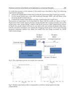
Fig. 1. The choice of initial population per iteration
 Stopping criterions of GA are the key factor of decreasing the computation burden. GA

is used to compute the control sequence. The objective value J(k+1) at the (k+1)-th
control interval is computed and compared with J(k) that stored at the k-th control
interval. If J(k+1) is smaller than J(k), that at the k-th control interval, then the control
sequence
u(k+1) is retained as a good feasible solution, and its first element u(k+1|k+1)
is sent to the plant. Otherwise, if there does not exist a feasible value for
u(k+1) to yield
J(k+1) < J(k), then the best
u(k+1) is chosen to decrease the objective function the most.
The traditional MPC approach requires the global solution of a nonlinear optimization
problem. This is in practice not achievable within finite computing time. An improved
NMPC algorithm based on GA does not necessarily depend on a global or even local
minimum. The optimizer provides a feasible decedent solution, instead of finding a global
or local minimum. The feasible solution decreases the cost function instead of minimizing
the cost function. Judicious selection of the termination criterions of GA is the key factor in
reducing the computation burden in the design of the suboptimal NMPC algorithm. To this
end, the following two strategies at the (k+1)-th step are proposed.
With the above two strategies, the computational complexity of the control calculation is
substantially reduced. Summarizing, our proposed improved NMPC algorithm performs
the following iterative steps:
Step 1. [Initialization]:
choose parameters P, X
F
, Q, R, Q’ and model x(k+1) = f(x(k),u(k)); initialize the state and
control variables at k = 0; compute and store J(0).
Step 2. [modified Iteration]:
 at the k-th control interval, determine the control sequence u(k) using GA satisfies
constraints (3b) (3c), terminal stability constraint (3d) and J(k) < J(k-1). The first input
u(k|k) is then sent into the plant.
 store J(k) and set k = k+1;

 if there does not exist a feasible value for u(k) to yield J(k) < J(k-1), then the best u(k) is
chosen to decrease the objective function the most.
Step 3. [Termination]
The entire calculation is repeated at subsequent control interval k+1 and goes to Step 2.
Though the proposed method does not seek a globally or locally optimal solution within
each iteration step, it may cause little performance degradation to the original GA due to its
iterative nature, which is known to be capable of improving suboptimal solution step by
step until reaching near-optimal performance at the final stage. Besides its near-optimal
performance, the proposed algorithm possesses salient feature; it guarantees overall system
stability and, most of all, leads to considerable reduction in the online computation burden.
Finding a control sequence that satisfies a set of constraints is significantly easier than
solving a global optimization problem. Here it is possible to obtain the suboptimal control

Improved Nonlinear Model Predictive Control Based on Genetic Algorithm

55
sequence via GA for practical systems with very demanding computation load, that is,
systems with a small sampling time or a large prediction horizon.
4. Stability of nonlinear model predictive control system
The closed-loop system controlled by the improved NMPC based on GA is proved to be
stable.
Theorem 1: For a system expressed in (1) and satisfying the assumption A1-A4, the closed-
loop system is stable under the improved NMPC framework.
Proof: Suppose there are an admissible control sequence
u(k) and a state sequence x(k) that
satisfy the input, state and terminal stability constraints at the sampling time k.
At the sampling time k, the performance index, which is related to
u(k) and x(k), is described
as

*
( ) ( ;u( ),x( ))Jk J k k k (6)
In the closed-loop system controlled by the improved NMPC, define the feasible input and
state sequences for the successive state are x
+
=f(x, u(k|k)).

u ( 1) [ ( 1| ), , ( 1| ), ( ( | )) ]
x ( 1) [ ( 1| ), , ( | ), ( ( | ), ( ( | ))) ]
TT TT
F
TT TT
F
kukkukPkKxkPk
k x k k x k Pk fxk PkK xk Pk


   
    
(7)
The resulting objective function of
u(k+1) and x(k+1) at the (k+1)-th sampling time is
(1)(1;u(1),x(1))Jk Jk k k

    (8)
If the optimal solution is found, it follows that

** *
(1) () (1) ()
(, ()) ((, ())) () (, ())

PF F
Jk Jk Jk Jk
lxK x F
f
xK x Fx lxK x

  
   
(9)
From A4, the following inequality holds

**
(1) () (,())
P
Jk Jk lxKx 
(10)
Or using the improved NMPC algorithm, it follows that

** *
(1) () (1) ()0Jk Jk Jk Jk


 (11)
Thus the sequence
*
()Jki

over P time indices decreases. As such and given the fact that the
cost function
(,)lxu is lower-bounded by zero, it is evident that

*
()Jki

converges. Taking
the sum, we obtain

**
1
( ) ( ) [ ( ( ), ( ))]
P
i
Jk P Jk lxkiuk i

    

(12)
Also, because the sequence
*
()Jki

is decreasing, then as N ,we have
(( ),( )) 0lxk i uk i and 0x  . Hence, the closed-loop system is stable.

Advanced Model Predictive Control

56
5. Simulation and experiment results
5.1 Simulation results to a continuous stirred tank reactor plant
5.1.1 Model of continuous stirred tank reactor plant
Consider the highly nonlinear model of a chemical plant (continuous stirred tank reactor-

CSTR). Assuming a constant liquid volume, the CSTR for an exothermic, irreversible
reaction, A→B, is described by

/( )
0
/( )
0
()
() ()
ERT
AAfA A
ERT
fAC
PP
q
CCCkeC
V
q
HUA
TTT ke C TT
VC VC






  



(13)
where C
A
is the concentration of A in the reactor, T is the reactor temperature and T
c
is the
temperature of the coolant stream. The parameters are listed in the Table 1.

Variables Meaning Value Unit
q
the inlet flow 100 l/min
V
the reactor liquid volume 100 l
C
Af
the concentration of inlet flow 1 mol/l
k
0
reaction frequency factor 7.2*10
10
min-1
E/R
8750 K
E
activation energy
R
gas constant 8.3196*10
3
J/(mol K)
T

f
the temperature of inlet flow 350 K
∆H
the heat of reaction -5*10
4
J/mol
ρ
the density 1000 g/l
C
P
the specific heat capacity of the fluid 0.239 J/(g K)
UA
5*10
4
J/(min K)
U
the overall heat transfer coefficient
A
the heat transfer area
Table 1. List of the model parameters
5.1.2 Simulation results
The paper present CSTR simulated examples to confirm the main ideas of the paper. The
nominal conditions, C
A
= 0.5mol/l, T = 350K, T
c
= 300K, correspond to an unstable operating
point. The manipulated input and controlled output are the coolant temperature (T
c
) and

reactor temperature (T). And the following state and input constraints must be enforced:


2
|0 1,280 370
|280 370
A
A
CC
C
CT
T
TT













 
XR
UR
(14)

The simulation platform is MATLAB and simulation time is 120 sampling time. The
sampling time is Ts = 0.05s, mutation probability is P
c
=0.1, population size is 100, maximum
generation is 100, and the fitness value is 1/(J+1).

Improved Nonlinear Model Predictive Control Based on Genetic Algorithm

57
0 1 2 3 4 5 6
200
250
300
350
400
T, K


0 1 2 3 4 5 6
280
300
320
340
360
380
time, min
Tc, K
NMPC algorithm based on GAs
suboptimal NMPC algorithm based on GAs

Fig. 2. Comparative simulation between the conventional NMPC algorithm and the
suboptimal NMPC algorithm

method settling time, min percent overshoot,%
NMPC algorithm based on GA 0.75 1
Suboptimal NMPC algorithm based on GA 2.5 0
Table 2. Performance comparisons of simulation results

0 20 40 60 80 100 120
0
0.5
1
1.5
2
2.5
iterative time
consumption time , s


NMPC algorithm based on GAs
suboptimal NMPC algorithm based on GAs

Fig. 3. The time consumptions of the two methods

Advanced Model Predictive Control

58
For comparison, the same simulation setup is used to test both the conventional NMPC
algorithm based GA and the suboptimal NMPC algorithm. The resulting control values are
depicted in Fig 2. Table 2 compares the performance of the two algorithms using the metrics

settling time and percent of overshoot. The conventional NMPC algorithm has a faster
transient phase and a smaller percentage of overshoots.
When the population sizes or the maximum generation is relatively large, the time
consumption of the two methods is compared in Fig 3.
From Fig 2 and Table 2, it is apparent that the control performance of the two methods is
almost same. But from Fig 3, it is evident that the suboptimal NMPC algorithm based on GA
has a considerably reduced demand on computational complexity.
5.2 Simulation results to a coupled-tank system
5.2.1 Model of coupled-tank system
The apparatus
[15]
, see Fig.4, consists of two tanks T
1
and T
2
, a reservoir, a baffle valve V
1
and
an outlet valve V
2
. T
1
has an inlet commanded through a variable pump based on PMW and
T
2
has an outlet that can be adjusted through a manually controlled valve only. The outlets
communicate to a reservoir from which the pumps extract the water to deliver it to the tank.
The two tanks are connected through the baffle valve, which again can only be adjusted
manually. The objective of the control problem is to adjust the inlet flow so as to maintain
the water level of the second tank close to a desired setpoint.

The water levels h
1
and h
2
, which are translated through the pressure transducer into a DC
voltage ranging from 0V to 5V, are sent to PC port via A/D transition. The tank pump
control, which is computed by the controller in PC with the information of the water level h
1

and h
2
, is a current level in the range 4mA to 20mA, where these correspond to the pump not
operating at all, and full power respectively.


Fig. 4. Coupled-tank apparatus

Improved Nonlinear Model Predictive Control Based on Genetic Algorithm

59
The dynamics of the system are modeled by the state-space model equations:

1
12
2
12 20
input
dh
AQQ
dt

dh
AQQ
dt


(15)
where the flows obey Bernoulli’s equation
[16]
, i.e.

1/2
12 1 1 2 1 2
s
g
n( )(2 )QShhghh


(16)

1/2
20 2 2
(2 )QSgh

 (17)
and
1, 0
sgn( )
1, 0
z
z

z






is the symbol function of parameter z.
The output equation for the system is

2
y
h

(18)
The cross-section areas, i.e.
A and S, are determined from the diameter of the tanks and
pipes. The flow coefficients,
μ
1
and μ
2,
have experimentally (from steady-state
measurements) been determined. Table 3 is the meanings and values of all the parameters in
Eqn.15

Signal Physics Meaning Value
A
Cross-section area of tank 6.3585×10
-3

m
2
S
Cross-section area of pipe 6.3585×10
-5
m
2
g
acceleration of gravity 9.806m/s
2
μ
1
flow coefficient 1 0.3343
μ
2
flow coefficient 2 0.2751
Table 3. Meanings and value of all the parameters
Several constraints have to be considered. Limited pump capacity implies that values of
in
p
ut
Q range from 0 to 50cm
3
/s. The limits for the two tank levels, h
1
and h
2
,

are from 0 to

50
cm.
5.2.2 Simulation results
The goal of the couple-tank system is to control the level of Tank 2 to setpoint. The initial
levels of the two tanks,
h
1
, h
2
, are 0cm. The objectives and limits of the tank system: Input
constraint is 0≤
u≤100%; State objectives are 0≤h
1
, h
2
≤0.5m, and the setpoint of Tank 2 is 0.1m.
The simulation platform is MATLAB and simulation time is 80 sample time. In NMPC,
select prediction horizon
P=10, weighting parameters 8QQ

 , R=1, sample time Ts=5s,
mutation probability
Pc=0.1, population size is 200, maximum generation is 100, the fitness
value is 1/(
J+1).

Advanced Model Predictive Control

60
For the purpose of comparison the same simulation is carried out with the conventional

NMPC algorithm based GA and the fast NMPC algorithm. The result is shown in Fig 5. The
performance indexes of the two algorithms are shown in Table 4.






Fig. 5. Compared simulation results based on conventional NMPC and fast NMPC
algorithm



method Settling time,
s percent overshoot, %
NMPC algorithm based on GA 70 3
Fast NMPC algorithm based on GA 100 7

Table 4. Performance index of simulation results
When the population sizes or the maximum generation is relatively larger, the time
consumptions of the two method is shown in Fig 6.

Improved Nonlinear Model Predictive Control Based on Genetic Algorithm

61
From Fig 5 and Table 4, it is apparent that the control performance of the two methods is
almost same. But from Fig 6, the computation demand reduces sign
ificant when the fast
NMPC algorithm based on GA is brought into the system.
5.2.3 Experiment results

The objectives and limits of the system: Input constraint is 0≤u≤100%; State objectives are
0≤h
1
,h
2
≤0.5m, and the setpoint of Tank 2 is 0.1m. Select prediction horizon P=10, weighting
parameters
8QQ, R=1, sample time Ts=5s, mutation probability Pc=0.1, population size
is 200, maximum generation is 100.
The tank apparatus is controlled with the NMPC algorithm based on conventional GA, the
experimental curve is shown in Fig 7 and performance index is shown in Table 5.











Fig. 6. Time consumptions for two methods

Advanced Model Predictive Control

62

Fig. 7. Experimental curve of NMPC based on GA




Time, s 0-400 401-800 801-1200
Setpoint, m 0.1 0.15 0.07
Settling time, s 159 190 210
Percent overshoot None None None


Table 5. Performance index of experimental result with conventional NMPC
The same experiment is carried out with fast NMPC algorithm based on GA. The result is
shown in Fig 8 and performance index is shown in Table 5.

Improved Nonlinear Model Predictive Control Based on Genetic Algorithm

63

Fig. 8. Experimental curve of fast NMPC based on GA

Time, s 0-400 401-800 801-1200
Set
p
oint, m 0.1 0.15 0.07

Settlin
g
time, s 190 190 260
Percent overshoot None None None
Table 6. Performance index of experimental result with fast NMPC
6. Conclusions
In this paper an improved NMPC algorithm based on GA has been proposed. The aim is to
reduce the computational burden without much deterioration to the control performance.
Compared with traditional NMPC controller, our approach has much lower computational
burden, which makes it practical to operate in systems with a small sampling time or a large
prediction horizon.
The proposed approach has been tested in CSTR and a real-time tank system. Both
computer simulations and experimental testing confirm that the suboptimal NMPC based
on GA resulted in a controller with less computation time.
7. Acknowledgment
This work is supported by National Natural Science Foundation of China (Youth
Foundation, No. 61004082) and Special Foundation for Ph. D. of Hefei University of
Technology (No. 2010HGBZ0616).

Advanced Model Predictive Control

64
8. References
Michael A.Henson, Nonlinear model predictive control: current status and future directions
[J], Computers and Chemical Engineering 23(1998):187-202
D.Q.Mayne, J.B.Rawlings, C.V.Rao and P.O.M.Scokaert, Constrained model predictive
control: Stability and optimality [J], Automatica 36(2000): 789-814
S.Joe Qin and Thomas A.Badgwell, a survey of industrial model predictive control
technology [J], Control Engineering Practice 11(2003): 733-764
Mark Cannon, Efficient nonlinear model predictive control algorithms [J], Annual Reviews

in Control 28(2004): 229-237
Basil Kouvaritakis and Mark Cannon, Nonlinear predictive control: Theory and practice
[M], the institution of electrical engineers, 2001
Frode Martinse, Lorenz T.Biegler and Bjarne A.Foss, A new optimization algorithm with
application to nonlinear MPC[J], Journal of Process Control, 2004:853-865
Moritz Diehl, Rolf Findeisen, Frank Allgower, Hans Georg Bock and Johannes Schloder,
stability of nonlinear model predictive control in the presence of errors due to
numerical online optimization, Proceedings of the 42nd IEEE Conference Decision
and Control, December 2003: 1419-1424
Rolf Findeisen, Moritz Diehl, Ilknur Disli-Uslu and Stefan Schwarzkopf, Computation and
Performance Assessment of Nonlinear Model Predictive Control[J]. Proc. Of the
41st IEEE Conference on Decision and Control December 2002:4613-4618
Moritz Diehl, Rolf Findeisen, Stefan Schwarzkopf, An efficient algorithm for nonlinear
predictive control of large-scale systems, Automatic Technology, 2002:557-567
L.T.Biegler, Advaneces in nonlinear programming concepts for process control, Proc. Cont.
Vol.8, Nos.5-6, pp.301-311, 1998
Alex Zheng and Frank Allgower, towards a practical nonlinear predictive control algorithm
with guaranteed stability for large-scale systems, Proceedings of the American
Control Conference, 1998:2534-2538
Jianjun Yang, Min Liu, Cheng Wu. Genetic Algorithm Based on Nonlinear Model Predictive
Control Method [J]. Control and Decision. 2003,2(18):141-144.
Fuzhen Xue, Yuyu Tang, Jie Bai. An Algorithm of Nonlinear Model Predictive Control
Based on BP Network [J]. Journal of University of Science and Technology of
China. 2004, 5(34): 593-598.
H.Michalska and D.Q.Mayne, robust receding horizon control of constrained nonlinear
systems, IEEE Transactions on Automatic Control, Vol.38, No.11,1993:1623-1633
Wei Chen, Gang Wu. Nonlinear Modeling of Two-Tank System and Its Nonlinear Model
Predictive Control [A]. Proceedings of the 24th Chinese Control Conference. 2005,
7:396-301
E.John Finnemore and Joseph B.Franzini, Fluid Mechanics with Engineering

Applications(Tenth Edition)[M], March 2003
N.K.Poulsen, B.Kouvaritakis and M.Cannon, Nonlinear constrained predictive control
applied to a coupled-tank apparatus[J], IEE Proc Control Theory Appl., Vol.148,
No 1, January 2001:17-24
Rolf Findeisen, Moritz Diehl, Ilknur Disli-Uslu and Stefan Schwarzkopf, Computation and
Performance Assessment of Nonlinear Model Predictive Control[J]. Proc. Of the
41st IEEE Conference on Decision and Control December 2002:4613-4618
0
Distributed Model Predictive Control
Based on Dynamic Games
Guido Sanchez
1
, Leonardo Giovanini
2
, Marina Murillo
3
and Alejandro Limache
4
1,2
Research Center for Signals, Systems and Computational Intelligence
Faculty of Engineering and Water Sciences, Universidad Nacional del Litoral
3,4
International Center for Computer Methods in Engineering
Faculty of Engineering and Water Sciences, Universidad Nacional del Litoral
Argentina
1. Introduction
Model predictive control (MPC) is widely recognized as a high performance, yet practical,
control technology. This model-based control strategy solves at each sample a discrete-time
optimal control problem over a finite horizon, producing a control input sequence. An
attractive attribute of MPC technology is its ability to systematically account for system

constraints. The theory of MPC for linear systems is well developed; all aspects such
as stability, robustness,feasibility and optimality have been extensively discussed in the
literature (see, e.g., (Bemporad & Morari, 1999; Kouvaritakis & Cannon, 2001; Maciejowski,
2002; Mayne et al., 2000)). The effectiveness of MPC depends on model accuracy and the
availability of fast computational resources. These requirements limit the application base for
MPC. Even though, applications abound in process industries (Camacho & Bordons, 2004),
manufacturing (Braun et al., 2003), supply chains (Perea-Lopez et al., 2003), among others, are
becoming more widespread.
Two common paradigms for solving system-wide MPC calculations are centralised and
decentralised strategies. Centralised strategies may arise from the desire to operate the
system in an optimal fashion, whereas decentralised MPC control structures can result from
the incremental roll-out of the system development. An effective centralised MPC can be
difficult, if not impossible to implement in large-scale systems (Kumar & Daoutidis, 2002;
Lu, 2003). In decentralised strategies, the system-wide MPC problem is decomposed into
subproblems by taking advantage of the system structure, and then, these subproblems
are solved independently. In general, decentralised schemes approximate the interactions
between subsystems and treat inputs in other subsystems as external disturbances. This
assumption leads to a poor system performance (Sandell Jr et al., 1978; Šiljak, 1996). Therefore,
there is a need for a cross-functional integration between the decentralised controllers, in
which a coordination level performs steady-state target calculation for decentralised controller
(Aguilera & Marchetti, 1998; Aske et al., 2008; Cheng et al., 2007; 2008; Zhu & Henson, 2002).
Several distributed MPC formulations are available in the literature. A distributed MPC
framework was proposed by Dumbar and Murray (Dunbar & Murray, 2006) for the class
4
2 Will-be-set-by-IN-TECH
of systems that have independent subsystem dynamic but link through their cost functions
and constraints. Then, Dumbar (Dunbar, 2007) proposed an extension of this framework that
handles systems with weakly interacting dynamics. Stability is guaranteed through the use of
a consistency constraint that forces the predicted and assumed input trajectories to be close to
each other. The resulting performance is different from centralised implementations in most

of cases. Distributed MPC algorithms for unconstrained and LTI systems were proposed in
(Camponogara et al., 2002; Jia & Krogh, 2001; Vaccarini et al., 2009; Zhang & Li, 2007). In (Jia
& Krogh, 2001) and (Camponogara et al., 2002) the evolution of the states of each subsystem
is assumed to be only influenced by the states of interacting subsystems and local inputs,
while these restrictions were removed in (Jia & Krogh, 2002; Vaccarini et al., 2009; Zhang &
Li, 2007). This choice of modelling restricts the system where the algorithm can be applied,
because in many cases the evolution of states is also influenced by the inputs of interconnected
subsystems. More critically for these frameworks is the fact that subsystems-based MPCsonly
know the cost functions and constraints of their subsystem. However, stability and optimality
as well as the effect of communication failures has not been established.
The distributed model predictive control problem from a game theory perspective for LTI
systems with general dynamical couplings, and the presence of convex coupled constraints
is addressed. The original centralised optimisation problem is transformed in a dynamic
game of a number of local optimisation problems, which are solved using the relevant
decision variables of each subsystem and exchanging information in order to coordinate
their decisions. The relevance of proposed distributed control scheme is to reduce the
computational burden and avoid the organizational obstacles associated with centralised
implementations, while retains its properties (stability, optimality, feasibility). In this context,
the type of coordination that can be achieved is determined by the connectivity and capacity of
the communication network as well as the information available of system’s cost function and
constraints. In this work we will assume that the connectivity of the communication network
is sufficient for the subsystems to obtain information of all variables that appear in their local
problems. We will show that when system’s cost function and constraints are known by all
distributed controllers, the solution of the iterative process converge to the centralised MPC
solution. This means that properties (stability, optimality, feasibility) of the solution obtained
using the distributed implementation are the same ones of the solution obtained using the
centralised implementation. Finally, the effects of communication failures on the system’s
properties (convergence, stability and performance) are studied. We will show the effect of
the system partition and communication on convergence and stability, and we will find a
upper bound of the system performance.

2. Distributed Model Predictive Control
2.1 Model Pr edictive Control
MPC is formulated as solving an on-line open loop optimal control problem in a receding
horizon style. Using the current state x
(k),aninputsequenceU(k ) is calculated to minimize
aperformanceindexJ
(
x(k), U(k)
)
while satisfying some specified constraints. The first
element of the sequence u
(k, k) is taken as controller output, then the control and the
prediction horizons recede ahead by one step at next sampling time. The new measurements
are taken to compensate for unmeasured disturbances, which cause the system output to be
66
Advanced Model Predictive Control
Distributed Model Predictive Control
BasedonDynamicGames 3
different from its prediction. At instant k, the controller solves the optimisation problem
min
U(k)
J
(
x(k), U(k)
)
st. (1)
X
(k + 1)=Γx(k)+HU(k)
U(k) ∈U
where Γ and H are the observability and Haenkel matrices of the system (Maciejowski, 2002)

and the states and input trajectories at time k are given by
X
(k)=
[
x(k, k) ··· x(k + V, k)
]
T
V > M,
U
(k)=
[
u( k, k) ··· u(k + M, k)
]
T
.
The integers V and M denote the prediction and control horizon. The variables x
(k + i, k) and
u
(k + i, k) are the predicted state and input at time k + i based on the information at time k
and system model
x
(k + 1)=Ax(k)+Bu(k),(2)
where x
(k) ∈ R
n
x
and u(k) ∈U⊆R
n
u
. The set of global admissible controls U =

{
u ∈ R
n
u
|Du ≤ d, d > 0
}
is assumed to be non-empty, compact and convex set containing the origin in
its interior.
Remark 1. The centralised model defined in (2) is more general than the so-called composite model
employed in (Venkat et al., 2008), which requires the states of subsystems to be decoupled and allows
only couplings in inputs. In this approach, the centralised model can represent both couplings in states
and inputs.
In the optimisation problem (1), the performance index J
(
x(k), U(k)
)
measures of the
difference between the predicted and the desired future behaviours. Generally, the quadratic
index
J
(
x(k), U(k)
)
=
V
∑
i=0
x
T
(k + i, k)Q

i
x(k + i, k)+
M
∑
i=0
u
T
(k + i, k)R
i
u( k + i, k) (3)
is commonly employed in the literature. To guarantee the closed–loop stability, the weighting
matrices satisfy Q
i
= Q > 0, R
i
= R > 0 ∀i ≤ M and Q
i
=
¯
Q
∀i > M,where
¯
Q is given by
A
T
¯
QA
−
¯
Q

= −Q (Maciejowski, 2002). For this choice of the weighting matrices, the index
(3) is equivalent to a performance index with an infinite horizon.
J
∞
(
x(k), U(k)
)
=
∞
∑
i=0
x
T
(k + i, k)Qx(k + i, k)+u
T
(k + i, k)Ru(k + i, k).
In many formulations an extra constraint or extra control modes are included into (1) to ensure
the stability of the closed-loop system (Maciejowski, 2002; Rossiter, 2003).
2.2 Distributed MPC framework
Large-scale systems are generally composed of several interacting subsystems. The
interactions can either be: a) dynamic, in the sense that the states and inputs of each subsystem
influence the states of the ones to which it is connected, b) due to the fact that the subsystems
67
Distributed Model Predictive Control Based on Dynamic Games
4 Will-be-set-by-IN-TECH
share a common goal and constraint, or c) both. Systems of this type admit a decomposition
into m subsystems represented by
x
l
(k + 1)=

m
∑
p=1
A
lp
x
p
(k)+B
lj∈N
p
u
j∈N
p
(k) l = 1, ,m (4)
where x
l
∈ R
n
x
l
⊆ R
n
x
and u
l
∈U
l
⊆ R
n
u

l
⊂ R
n
u
are the local state and input respectively.
The set of control inputs indices of subsystem l is denoted
N
l
,andthesetI denotes all control
input indices such that u
(k)=u
j∈I
(k).
Remark 2. This is a very general model class for describing dynamical coupling between subsystems
and includes as a special case the combination of decentralised models an d interaction models in (Venkat
et al., 2008). The subsystems can share input variables such that
m
∑
l=1
n
u
l
≥ n
u
.(5)
Each subsystem is assumed to have local convex independent and coupled constraints, which
involve only a small number of the others subsystems. The set of local admissible controls
U
l
=

{
u
l
∈ R
n
u
l
| D
l
u
l
≤ d
l
, d
l
> 0
}
is also assumed to be non-empty, compact, convex set
containing the origin in their interior.
The proposed control framework is based on a set of m independent agents implementing a
small-scale optimizations for the subsystems, connected through a communication network
such that they can share the common resources and coordinate each other in order to
accomplish the control objectives.
Assumption 1. The local states of each subsystem x
l
(k) are accessible.
Assumption 2. The communication between the control agents is synchronous.
Assumption 3. Control agents communicates several times within a sampling time interval.
This set of assumption is not restrictive. In fact, if the local states are not accessible they
can be estimated from local outputs y

l
(k) and control inputs using a Kalman filter, therefore
Assumption 1 is reasonable. As well, Assumptions 2 and 3 are not so strong because in
process control the sampling time interval is longer with respect the computational and the
communication times.
Under these assumptions and the decomposition, the cost function (3) can be written as
follows
J
(
x(k), U(k), A
)
=
m
∑
l=1
α
l
J
l

x
(k), U
j∈N
l
(k), U
j∈I−N
l
(k)

,(6)

where A
=
[
α
l
]
, α
l
≥ 0,
∑
m
l
=1
α
l
= 1, U
j
(k) is the j-th system input trajectory. This
decomposition of the cost function and input variable leads to a decomposition (1) into m
coupled optimisation problems
min
U
j∈N
l
(k)
J
(
x(k), U(k), A
)
68

Advanced Model Predictive Control
Distributed Model Predictive Control
BasedonDynamicGames 5
st.
X
(k + 1)=Γx(k)+HU(k) (7)
U
j∈N
l
(k) ∈U
j∈N
l
U
j∈I−N
l
(k) ∈ U
j∈I−N
l
where U
j∈I−N
l
denotes the assumed inputs of others agents. The goal of the decomposition is
to reduce the complexity of the optimisation problem (1) by ensuring that subproblems (7) are
smaller than the original problem (fewer decision variables and constraints), while they retain
the properties of the original problem. The price paid to simplify the optimisation problem (1)
is the needs of coordination between the subproblems (7) during their solution. In this way,
the optimisation problem (1) has been transformed into a dynamic game of m agents where each
one searches for their optimal decisions through a sequence of strategic games,inresponseto
decisions of other agents.
Definition 1. A dynamic game


m, U, J
l
(
x(k), U
q
(k), A
)
, D(q, k)

models the interaction of m
agents over iterations q and is composed of: i) m
∈ N agents; ii) a non empty set U that corresponds
to the available decisions U
q
l
(k) for each agent; iii) an utility function J
l
(
x(k), U
q
(k), A
)
: x(k) ×
U
q
(k) → R
+
for each agent; iv) an strategic game G(q, k) that models the interactions between agents
at iteration q and time k; v) a dynamic process of decision adjustment

D(q, k) :
(
U
q
(k), G(q, k), q
)
→
U
q +1
(k).
At each stage of the dynamic game, the joint decision of all agents will determine the outcome
of the strategic game
G(q, k) and each agent has some preference U
q
j
∈N
l
(k) over the set of
possible outcomes
U. Based on these outcomes and the adjustment process D(q, k) ,which
in this framework depends on the cost function J
l
(· ) and constraints, the agents reconcile
their decisions. More formally, a strategic game is defined as follows (Osborne & Rubinstein,
1994)
Definition 2. A finite strategic game
G(q, k)=

m, U
l

, J
l
(
x(k), U
q
(k), A
)
models the interactions
between m agents and is composed of: i) a non empty finite set
U
l
⊆Uthat corresponds the set
of available decisions for each agent; ii) an utility function J
l
(
x(k), U
q
(k), A
)
: x(k) × U
q
(k) →
R U
q
(k) ∈Ufor each agent.
In general, one is interested in determining the choices that agents will make when faced with
a particular game, which is sometimes referred to as the solution of the game. We will adopt
the most common solution concept, known as Nash equilibrium (Nash, 1951): a set of choices
where no individual agent can improve his utility by unilaterally changing his choice. More
formally, we have:

Definition 3. A group of control decisions U
(k) is said to be Nash optimal if
J
l

x
(k), U
q
j
∈N
l
(k), U
q −1
j
∈I−N
l
(k)

≤ J
l

x
(k), U
q −1
j
∈N
l
(k), U
q −1
j

∈I−N
l
(k)

where q
> 0 is the number of iterations elapsed during the iterative process.
If Nash optimal solution is achieved, each subproblem does not change its decision U
q
j
∈N
l
(k)
because it has achieved an equilibrium point of the coupling decision process; otherwise the
local performance index J
l
will degrade. Each subsystem optimizes its objective function
69
Distributed Model Predictive Control Based on Dynamic Games
6 Will-be-set-by-IN-TECH
using its own control decision U
q
j
∈N
l
(k) assuming that other subsystems’solutions U
q
j
∈I−N
l
(k)

are known. Since the mutual communication and the information exchange are adequately
taken into account, each subsystem solves its local optimisation problem provided that the
other subsystems’ solutions are known. Then, each agent compares the new solution with
that obtained in the previous iteration and checks the stopping condition



U
q
j
∈N
l
(k) − U
q −1
j
∈N
l
(k)



∞
≤ ε
l
l = 1, ,m.(8)
If the algorithm is convergent, condition (8) will be satisfied by all agents, and the whole
system will arrive to an equilibrium point. The subproblems m (7) can be solved using the
following iterative algorithm
Algorithm 1
Given Q

l
, R
l
,0< q
max
< ∞, ε
l
> 0 ∀l = 1, ··· , m
For each agent ll
= 1, ··· , m
Step 1 Initialize agent l
1.a Measure the local state x
l
(k), q = 1,
ρ
l
= φε
l
φ  1
1.bU
0
(k)=
[
u( k, k − 1) ··· u(k + M, k − 1) 0
]
Step 2 while ρ
l
> ε
l
and q < q

max
2.a Solve problem (7) to obtain
˜
U
q
j
∈N
l
(k)
2.b for p = 1, ··· , m and p = l
Communicate
˜
U
q
j
∈N
l
(k) to agent p
end
2.c Update the solution iterate q
∀j ∈N
l
U
q
j
(k)=
∑
m
p
=1

α
p
˜
U
q
i
∈N
p
∩j
(k)
+

1
−
∑
m
p
=1
α
p
card
(
j ∩N
l
)

U
q −1
j
(k)

2.d ρ
l
=



U
q
j
∈N
l
(k) − U
q −1
j
∈N
l
(k)



∞
q = q + 1
end
Step 3 Apply u
l
(k, k)
Step 4 k = k + 1andgotoStep1
At each k, q
max
represents a design limit on the number of iterates q and ε

l
represents the
stopping criteria of the iterative process. The user may choose to terminate Algorithm 1 prior
to these limits.
3. Properties of the framework
3.1 P erformance
Given the distributed scheme proposed in the previous Section, three fundamental questions
naturally arise: a) the behavior of agent’s iterates during the negotiation process, b)the
70
Advanced Model Predictive Control
Distributed Model Predictive Control
BasedonDynamicGames 7
location and number of equilibrium points of the distributed problem and c) the feasibility
of the solutions. One of the key factors in these questions is the effect of the cost function and
constraints employed by the distributed problems. Therefore, in a first stage we will explore
the effect of the performance index in the number and position of the equilibrium points.
Firstly, the optimality conditions for the centralised problem (1) are derived in order to have
a benchmark measure of distributed control schemes performance. In order to make easy the
comparison, the performance index (3) is decomposed into m components related with the
subsystems, like in the distributed problems (7), as follows
J
(
x(k), U(k), Θ
)
=
m
∑
l=1
θ
l

J
l
(
x(k), U(k)
)
, θ
l
≥ 0,
m
∑
l=1
θ
l
= 1. (9)
This way writing the performance index corresponds to multiobjective characterization of the
optimisation problem (1). Applying the first–order optimality conditions we obtain
m
∑
l=1
θ
l
∂J
l
(
x(k), U(k)
)
∂U
j∈N
p
(k)

+
λ
T
D
j∈N
p
= 0 p = 1, ,m, (10a)
λ
T

D
j∈N
p
U
j∈N
p
(k) − b

= 0, (10b)
where D
j
is the j–th column vector of D. The solution of this set of equations U
∗
(k) is the
optimal solution of the optimisation problem (1) and belongs to Pareto set,whichisdefinedas
(Haimes & Chankong, 1983).
Definition 4. AsolutionU
∗
(k) ∈Uis said to be Pareto optimal of the optimisation problem (1) if
there exists no other feasible solution

∀U(k) ∈Usuch that J
l
(
x(k), U(k)
)
≤ J
l
(
x(k), U
∗
(k)
)
∀l =
1, ,m.
In distributed control the agents coordinate their decisions, through a negotiation process.
Applying the first–order optimality conditions to decentralised cost (6) we obtain
m
∑
l=1
α
l
∂J
l
(
x(k), U(k)
)
∂U
j∈N
p
(k)

+
λ
T
D
j∈N
p
= 0 p = 1, ,m, (11a)
λ
T

D
j∈N
p
U
j∈N
p
(k) − b

= 0. (11b)
By simple inspection of (10) and (11) we can see that these equations have the same structure,
they only differ on the weights. Therefore, the location of the distributed schemes equilibrium
will depend on the selection of α
l
l = 1, ,m. There are two options:
•Ifα
l
= 1,α
p=l
= 0 the optimality condition (11) becomes
∂J

l
(
x(k), U(k)
)
∂U
j∈N
l
(k)
+
λ
T
D
j∈N
l
= 0 l = 1, ,m, (12a)
λ
T

D
j∈N
l
U
j∈N
l
(k) − b

= 0. (12b)
This condition only evaluates the effect of U
j∈N
l

,givenU
j∈I−N
l
, in subsystem l
without taking into account its effects in the remaining agents (selfish behavior). This
configuration of the distributed problem leads to an incomplete and perfect information
game that can achieve Nash optimal solutions for a pure strategy (Cournot equilibrium)
71
Distributed Model Predictive Control Based on Dynamic Games
8 Will-be-set-by-IN-TECH
(Osborne & Rubinstein, 1994). By simple comparison of (10) and (12) we can conclude
that the solution of this equations lies outside of the Pareto set (Dubey & Rogawski,
1990; Neck & Dockner, 1987). The reason of Nash equilibrium inefficiency lies in the fact
that the information of each agent decision variable effects’ on the remaining agents is
neglected (α
p=l
= 0 incomplete information game). Therefore, each agent minimizes their
performance index, accommodating the effects of other agents’ decisions, without taking
in account its effects on the rest of the system. Besides the lack of optimality, the number of
equilibrium points generated by the optimality condition (12) can grow with the number
of agents (Bade et al., 2007).
•Ifα
l
> 0 the optimality condition (11) becomes
m
∑
l=1
α
l
∂J

l
(
x(k), U(k)
)
∂U
j∈N
p
(k)
+
λ
T
D
j∈N
p
=0 p = 1, ,m (13a)
λ
T

D
j∈N
p
U
j∈N
p
(k) − b

=0. (13b)
This condition evaluates the effect of U
j∈N
l

,givenU
j∈I−N
l
, in the entire system, taking in
account the effect of interactions between the subsystems (cooperative behavior), leading
to a complete and perfect information game. By simple comparison of (10) and (13) it is
easy to see that these two equations have a similar structure, therefore we can conclude
that their solutions lie in the Pareto set. The position of distributed MPC solutions will
depend on the values of α
l
.Intheparticularcaseofα
l
= θ
l
l = 1, ,m the solution of
the centralised and distributed schemes are the same.
The value of weights α
l
l = 1, ,m depends on the information structure; that is the
information of the cost function and constraints available in each agent. If the cost function
and constraints of each agent are known by all the others, for example a retailer company,
α
l
can be chosen like the second distributed scheme (α
l
> 0 ∀l = 1, ,m). In this
case the centralised optimisation problem is distributed between m independent agents that
coordinate their solutions in order to solve the optimisation problem in a distributed way. For
this reason we call this control scheme distributed MPC. On the other case, when the local
cost function and constraints are only known by the agents, for example a power network

where several companies compete, the weights α
l
should be chosen like the first scheme
(α
l
= 1, α
p=l
= 0 ∀l, p = 1, ,m). In this case the centralised optimisation problem is
decentralised into m independent agents that only coordinate the effects of their decisions to
minimize the effect of interactions. For this reason we call this control scheme coordinated
decentralised MPC.
Remark 3. The fact that agents individually achieve Nash optimality does not imply the global
optimality of the solution. This relationship will depend on the structure of agents’ cost function and
constraints, which depends on the value of weights α
l
, and the number of iterations allowed.
The structure of U
j∈N
l
determine the structure of constraints that can be handled by the
distributed schemes. If the subproblems share the input variables involved in the coupled
constraints (
N
l
∩N
p=l
= ∅), the distributed MPC schemes can solve optimisation problems
with coupled constraints. On the other hand, when subproblems do not include the input
variables of coupled constraints (
N

l
∩N
p=l
= ∅), the distributed MPC schemes can only
solves optimisation problems with independent constraints (Dunbar, 2007; Jia & Krogh, 2001;
Venkat et al., 2008). These facts become apparent from optimality conditions (12) and (13).
72
Advanced Model Predictive Control
Distributed Model Predictive Control
BasedonDynamicGames 9
3.2 Convergence
During the operation of the system, the subproblems (7) can compete or cooperate in the
solution of the global problem. The behavior of each agent will depend on the existence,
or not, of conflictive goals that can emerge from the characteristics of the interactions, the
control goals and constraints. The way how the system is decomposed is one of the factors
that defines the behavior of the distributed problem during the iterations, since it defines how
the interactions will be addressed by distributed schemes.
The global system can be partitioned according to either the physical system structure or
on the basis of an analysis of the mathematical model, or a combination of both. Heuristic
procedures for the partitioning the system based on input–output analysis (see (Goodwin
et al., 2005; Henten & Bontsema, 2009; Hovd & Skogestad, 1994)), an state–space analysis
based (see (Salgado & Conley, 2004; Wittenmark & Salgado, 2002) or on performance metric
for optimal partitioning of distributed and hierarchical control systems (see (Jamoom et al.,
2002; Motee & Sayyar-Rodsari, 2003)) have been proposed. In all these approaches the
objective is to simplify the control design by reducing the dynamic couplings, such that the
computational requirements are evenly distributed to avoid excessive communication load.
It is important to note that the partitioning of a state–space model can lead to overlapping
states both due to coupled dynamics in the actual continuous system and due to discrete-time
sampling, which can change the sparsity structure in the model.
Assumption 4. The model employed by the distributed MPC algorithms are partitioned following the

procedures described in (Motee & Sayyar-Rodsari, 2003).
To analysed the effect of the system decomposition on the distributed constrained scheme,
firstly we will analysed its effects on unconstrained problem. Solving the optimality condition
(11) for an unconstrained system leads to
U
q
(k)=K
0
U
q −1
(k)+K
1
x(k) ∀q > 0, (14)
which models the behavior of the distributed problem during the iterative process. Its stability
induces the convergence of the iterative process and it is given by
|
λ
(
K
0
)|
<
1. (15)
The gain
K
1
is the decentralised controller that computes the contribution of x(k) to U(k) and
has only non–zero elements on its main diagonal
K
1

=
[
K
ll
]
l = 1, ,m. On other hand,
K
0
models the interaction between subsystems during the iterative process, determining its
stability, and has non zero elements on its off diagonal elements
K
0
=
⎡
⎢
⎢
⎢
⎣
0
K
12
··· K
1m
K
21
0 K
2m
.
.
.

.
.
.
.
.
.
K
m1
··· K
mm−1
0
⎤
⎥
⎥
⎥
⎦
. (16)
The structure of the components of
K
0
and K
1
depends on the value of the weights α
l
:
•Ifthecoordinated decentralised MPC is adopted (α
l
= 1, α
p=l
= 0) the elements of K

0
are
given by given by
K
lp
= −K
ll
H
lp
l, p = 1, ,m (17)
73
Distributed Model Predictive Control Based on Dynamic Games