Advances in Modern Woven Fabrics Technology Part 5 pdf

Finite Element Modeling of Woven Fabric Composites at
Meso-Level Under Combined Loading Modes

69

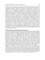
Fig. 4. The X-ray image from cross section of fibrous yarns (top) before loading; (bottom)
after loading (Badel et al., 2008)
to arrive at strain-dependant relationships for the yarns’ transverse stiffness parameters
(Gasser et al., 2000; Badel et al., 2008).
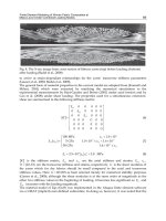
The general form of material properties in the current model are adapted from (Komeili and
Milani, 2010) which were extracted by matching the numerical simulations to the
experimental measurements by Buet-Gautier and Boisse (2001) under axial tension and by
Cao et al. (2008) under shear loading. The properties used for a simultaneous extension-
shear are summarized in the following stiffness matrix:


11
22
33
0 0 000
0 0 000
0 0 000
000 0 0
000 0 0
000 0 0
E
E
E
G
G
G






















C
(6)


3
11
33
11 11 11
3

11
100MPa 1.0 10
5GPa1.0 10 1.6 10
50GPa1.6 10
E














(7)

52
11
2.5 10 3.0MPa
tt tt
E

  (8)



C
is the stiffness matrix,
11
E and
11

are the axial stiffness and strains;
tt
E ,
tt

,
{22,33}tt  are the transverse stiffness and strains, respectively. G is the shear modulus of
the yarns which for dry fabrics should be small compared to the axial and transverse
stiffness values. Here 60GMPa

as been selected merely for numerical stability purposes
(Gasser et al., 2000); although the shear modulus is at the same order of magnitude as the
other two stiffness values in the beginning of loading, it becomes less significant as
11
E and
22

E increases with the loading magnitude.
The material model of Eqs (6)-(8) was implemented in the Abaqus finite element software
via a UMAT (implicit) user-defined subroutine. In doing so, however, it was noted that the

Advances in Modern Woven Fabrics Technology

70

large difference between the stiffness in the yarn axial direction compared to the transverse
and shear stiffness values highlights the extreme importance of applying proper material
orientation updates during loading steps. The point is that the material properties should be
defined in a frame which is rotating with the fiber direction in the yarns. On the other hand,
conventional methods in the finite element codes use other (e.g., Green & Naghdi, 1965;
Jaumann, 1911) methods for updating the material orientation under large deformation. The
problem can be handled with user-defined material subroutines. Subsequently, two
approaches may be implemented to ensure that the material properties during stress
updates is based on the frame attached to the fibers: (1) Either the stiffness matrix defined
along the fiber direction can be transformed to the current working frame of the finite
element software, or (2) the stress in the working frame of the software can be transformed
to the frame of the fiber and transformed back to the working frame after applying the stress
updates in the fiber frame. The details of each method are available in (Badel et al., 2008)
and (Komeili and Milani, 2010); the former reference employed an explicit and the latter
reference an implicit integrator.
2.3 Periodic boundary conditions
A single isolated unit cell cannot be considered as a good representative of the whole fabric
structure unless the effect of adjacent cells is taken into account. In other words, suitable
kinematic (or dynamic) conditions should be applied on the perimeter of the unit cell where
it is attached to the adjacent cells. These conditions are often called periodic boundary
conditions. They are very similar (though different) to symmetric boundary conditions. A
thorough discussion on their mathematical details and implementation under individual
loading modes is given in (Badel et al., 2007).
The method that has been used in this study is based on the periodic boundary conditions
reported in (Peng and Cao, 2002). According to their work, the side surfaces of yarns should
remain plane and normal to the unit cell mid surface during deformation. More details of
the latter kinematic conditions on unit cells are also given in (Komeili and Milani 2010).
2.4 Loading boundary conditions
There is a variety of test setups used for the axial tension and shear testing of woven fabrics
(Buet-Gautier and Boisse, 2001; Cao et al., 2008). On the other hand, experimental setups for

the combined loading modes are new and limited. First, it should be defined how a
combined loading mode is exerted on a fabric specimen. For example, having a bi-axial load
on a fabric where the axial loads does not rotate with the rotation of the yarns and stays
parallel to its original direction during deformation, even after the shear load is applied,
may be considered a special case of combined loading. As another example, one may
consider a combined loading condition where the direction of the axial load rotates and
realigns along the yarn direction. For a practical analysis of fabrics, the latter case of
stretching in the yarn direction is more important than the former case of stretching yarns
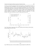
along a (fixed) off-axis direction (Boisse 2010). A new test setup capable of applying
combined loading in the form of shear and biaxial stretching along the yarns (Figure 5) has
been developed in (Cavallaro et al., 2007).
In order to simulate the unit cell of the fabric under such combined loading in the
aforementioned Abaqus model, a set of kinematic couplings were applied around the unit
cell to satisfy the periodic boundary conditions. Namely, the shear loading has been applied


Finite Element Modeling of Woven Fabric Composites at
Meso-Level Under Combined Loading Modes

71

Fig. 5. Experimental fixture for applying combined shear and axial tension on fabrics
(Cavallaro et al., 2007).
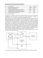
via rotation on one of the yarn sides and the rest of unit cell boundaries have linked to
follow this movement through a periodic boundary condition. For the axial tension,
connector elements between the two corners of each side yarn have been used (they can be
seen as solid lines around the unit cell in Figure 6). The connector elements are chosen from
the Abaqus library and provide an axial degree-of-freedom between their reference nodes.
The axial distance between the nodes can be changed to apply/simulate stretching on the
yarns. The reference points are not part of the yarns geometry, but they are kinematically

connected to the nodes on the cross sectional surfaces of yarns (i.e., the side surfaces of the
unit cell) to implement the periodic and loading boundary conditions. Moreover, there are
four reference points on the mid-points of the side lines to impose the kinematic conditions
on the middle yarns. The latter reference points are also connected to the corner points by
kinematic constraints. Figure 6 shows the aforementioned conditions schematically.
Eventually, the material resistance to deformation in the form of reaction moment from the
rotation boundary condition and the normal force from the axial connector elements are

Advances in Modern Woven Fabrics Technology

72
calculated and reported in the post processing of simulations. They can then be used in the
normalized form and compared with experimental results.


Axial tension along x
1
Axial tension along x
2
In-plane rotation
x
1
x
2
Middle yarns

Fig. 6. The loading boundary conditions used on the unit cell to model the deformation
under a combined loading mode; Circles show the location of reference points.
3. A preliminary validation
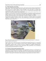
In order to validate the model with the existing data in the literature, it is compared to two

basic cases where the unit cell is under pure bi-axial tension and shear (Komeili and Milani,
2010). Figure 7 shows the results of these comparisons. In the same figure, a set of actual
picture frame test data, collected at the Hong Kong University of Science and Technology
(HKUST), is replicated from (Cao et al., 2008). For the axial mode, however, data with the
same unit cell geometrical parameters was not available. The differences between the
resultant forces and moments in each mode can be related to the type of the unit cell used,
shear stiffness of yarns, the method of applying boundary/loading conditions, and other
details of the two finite element models in controlling their convergence (e.g. hourglass
stiffness, mesh size, etc). In addition, one may redo the inverse identification of the yarn
model using the current model. However, as the main goal of this chapter is to highlight the
relative effect of combined loading on the mechanical characterization of woven fabrics (i.e.,
Finite Element Modeling of Woven Fabric Composites at
Meso-Level Under Combined Loading Modes

73
compared to the individual deformation modes), the current model and material properties
are used without a loss of generality of the approach.

0
0.2
0.4
0.6
0.8
1
1.2
1.4
1.6
1.8
2
0 0.0005 0.001 0.0015 0.002

Reaction force (N/mm)
Axial strain
Bi-axial tension
Current model
Komeili and Milani 2010
0
0.005
0.01
0.015
0.02
0.025
0.03
0.035
0.04
0 102030
Torque (N.mm/mm^2)
Shear angle
Pure shear
Current model
Komeili and Milani 2010
HKUST (Cao et al., 2008)

(a) (b)
Fig. 7. A validation of the current model under (a) pure bi-axial and (b) shear mode.
4. The effect of combined loading
In this section the effect of combined loading on the response of the material is analysed,
when compared to those obtained from the individual biaxial and shear modes under the
same loading magnitude. Figure 8 shows the effect of combined loading on the reaction
force in the bi-axial tension and the reaction moment under shear loading. The amount of
normalized reaction moment while the fabric is under combined loading has increased up to

four times. It has also caused ~12% higher axial reaction force under an identical stretching
magnitude.

0
0.01
0.02
0.03
0.04
0.05
0.06
0 102030
Torque (N.mm/mm^2)
Shear angle
Shear
Combined
Pure shear
0
0.2
0.4
0.6
0.8
1
1.2
1.4
1.6
1.8
2
0 0.0005 0.001 0.0015 0.002
Reaction force (N/mm)
Axial strain

Bi-axial tension
Combined
Pure axial

(a) (b)
Fig. 8. The effect of combined loading on the reaction force and moment when compared to
the individual (a) shear and (b) biaxial modes. The difference between curves in each graph
indicates the presence of additional local deformation phenomena/ interactions between
shear and axial modes under combined loading.

Advances in Modern Woven Fabrics Technology

74
The obtained numerical results from bi-axial loading well agree with what has been
suggested through experimental measurements in the literature. Namely, Boisse, et al.
(2001) and Buet-Gautier and Boisse (2001) argued that the effect of shear strain on the axial
behaviour of plain fabrics is not considerable. In other words, it may be concluded that the
small effect of shear deformation on the axial behaviour (~12%) can be considered as an
inherent material noise in the experimental data. On the other hand, Cavallaro et al. (2007)
reported that having the yarns under pretension in axial direction can greatly affect the
subsequent shear behaviour of the fabrics, which is in fact the case from the simulation
results in Figure 8.
After assessing the effect of combined loading on the basic normal and shear response of the
fabric, another important notion may be studied. The question is, “Does the sequence of
loading steps affect the response too?” In other words, if the axial loading is applied first,
followed by the shear loading, or vice versa, are the resultant reaction force and moments
the same as those when the two loadings are applied simultaneously?
To study the latter effect, let us define a normalized loading parameter

. It ranges from 0

to 1, where 0 refers to the initiation of loading and 1 represents the end of loading. For
example, during a simultaneous/combined loading:






; 
max max

 
 (9)
where

and

, are the shear angle and axial strain in each step of loading and
max

and
max

, are the corresponding maximum values. Similarly, for the shear loading followed by
the axial loading at

=
1
2
we have:

  
11

; 
22
max max
RR R



 
 

 
 

(10)
where,

2 0
0 0
xx
Rx
x








For the opposite case where the axial loading is followed by the shear loading, we may
write:

  
11

; 
22
max max
RRR

  

 
  

 
 

(11)
Results of the new simulations are presented in Figure 9. It can be clearly seen that for the
shear response, the sequence of the loading affects the resultant moment up to four times.
However, the axial response is still less sensitive to the effect of deformation from the shear
mode and the loading sequence. The results also indicate that if the shear deformation is
applied to the specimen first, the shear reaction moment is decreased substantially.
Moreover, during the step that the pure shear is applied, there seems to be a small reaction
force in the form of tension. This is perhaps due to the fact that during shearing, the sliding
of yarns on each other and their replacement in the fabric affect their waviness/crimp. In

Finite Element Modeling of Woven Fabric Composites at
Meso-Level Under Combined Loading Modes

75
turn, the crimp interchange would induce a small axial stretch in some regions of yarns,
especially if they are constrained at their ends (like in the picture frame test).

0
0.01
0.02
0.03
0.04
0.05
0.06
0.07
0.08
0.09
00.20.40.60.81
Torque (N.mm/mm^2)
Loading coefficient (α)
Shear
Simultaneous
Shear+Axial
Axial+Shear
0
0.5
1
1.5
2
2.5

0 0.2 0.4 0.6 0.8 1
Reaction force (N/mm)
Loading coefficient (α)
Bi-axial tension
Simultaneous
Shear+Axial
Axial+Shear

(a) (b)
Fig. 9. The effect of loading sequence on the response of (a) shear and (b) axial deformation;
the second loading step is applied after the dashed line for Axial+Shear and Shear+Axial
cases.
The results in Figure 9 can also be linked to the constitutive model of yarns. Recalling Eq.
(8), the transverse stiffness is a function of yarns’ axial and transverse strains (crushing
formula). The bi-axial stretching induces axial strain in the yarns, which leads to an increase
in the yarns’ transverse stiffness. In turn, the normal contact forces at the yarns cross over
regions are increased, leading to a higher contribution from friction to the total reaction
force. However, the opposite effect is not true. Under the bi-axial mode, the shear
deformation (before locking point) does not induce considerable axial and transverse
stretches in the yarns. Previously, using a sensitivity analysis under individual deformation
modes, it was also reported by Komeili and Milani (2010) that the effect of transverse
stiffness on the fabric response in the shear mode is considerable whereas it is ignorable in
the bi-axial mode.
5. Summary
A numerical finite element model of a plain weave fabric unit cell at meso-level is
developed. The model is capable of simulating specimens under simultaneous axial loading
along the yarn directions and the fabric shearing. It can be a useful tool for predicting the
meso-level local deformation phenomena in woven fabrics under complex loading
conditions, as well as for developing equivalent material models at macro-level for fast
simulation of fabric forming processes. Two fundamental deformation modes (shear and

equi-biaxial stretching) are applied through two separate kinematics boundary conditions to
facilitate extracting the contributions from each mode on the total resultant force and
moment.
The analysis on the effect of combined loading has been conducted in two ways. First, the
force and moment response of the unit cell under a predefined combined loading with a
specific shear angle and axial strain is compared to those of the pure shear and axial modes.
It was of interest to see if there is any interaction effect between the fundamental axial and
shear deformation mechanisms when a combined loading is applied. Results showed that

Advances in Modern Woven Fabrics Technology

76
this interaction in fact exists and it has a dramatic effect on the ensuing reaction moment
response (shear rigidity), but it is less important for the axial reaction force. Second, the
effect of applying combined loading in two sequential steps was scrutinized. Again, the
shear deformation response showed high sensitivity to the sequence of loading if it is
applied before the axial deformation. Moreover, it was noted that during shear deformation
there is a small tension reaction force, even though no stretching is applied to the yarns. This
is perhaps due to the crimp interchanges along with the imposed boundary conditions on
the end surfaces of yarns.
In summary, the above mentioned results show a high level of nonlinear interactions
between the material response in the axial tension and shear modes. This can be directly
related to the geometrical nonlinearities that exist in woven fabrics at meso-level and the
effect of crimp interchanges during loading. After each stage of loading, the rearrangement
of yarns in the fabric and their interactions should occur before yarns can go through further
stretching/shearing. Under the combined loading, the crimp changes due to each loading
mode can affect the reaction from the other mode. If loads are applied in sequence (e.g.,
shear followed by biaxial tension), the crimp changes in each step can affect the global
response due to the effect from the previous loading step. Considerably different
magnitudes of the shear moment were found between two cases where the shear and bi-

axial deformations are applied at the same time and where the shear is applied after the
axial loading. This observation clearly showed the higher sensitivity of the shear response to
the crimp interchanges. On the contrary, because the axial reaction forces are more related to
the stretching in the yarns, the shear deformation has minor influence on their axial force
magnitudes. The effect of axial tension on increasing the transverse stiffness of yarns is
deemed to be the main reason for the presence of interactions between the axial tension and
shear deformation under combined loading modes. Further experimental and/or numerical
studies are needed to scrutinize and validate the reported effects.
6. Acknowledgment
The authors would like to acknowledge financial support from the Natural Sciences and
Engineering Research Council (NSERC) of Canada.
7. References
Badel, P, Vidalsalle, E, & Boisse, P (2007) Computational determination of in-plane shear
mechanical behaviour of textile composite reinforcements.
Computational Materials
Science
40: 439-448.
Badel, P, Vidalsalle, E, & Boisse, P (2008) Large deformation analysis of fibrous materials
using rate constitutive equations.
Computers & Structures 86: 1164-1175.
Badel, P, Vidalsalle, E, Maire, E, & Boisse, P (2008) Simulation and tomography analysis of
textile composite reinforcement deformation at the mesoscopic scale.
Composites
Science and Technology
68: 2433-2440.
Badel, P, Gauthier, S, Vidal-Sallé, E, & Boisse, P. (2009) Rate constitutive equations for
computational analyses of textile composite reinforcement mechanical behaviour
during forming.
Composites Part A: Applied Science and Manufacturing 40: 997-1007.
Finite Element Modeling of Woven Fabric Composites at

Meso-Level Under Combined Loading Modes

77
Boisse, P, Zouari, B, & Daniel, J (2006) Importance of in-plane shear rigidity in finite element
analyses of woven fabric composite preforming.
Composites Part A: Applied Science
and Manufacturing
37: 2201-2212.
Boisse, P, Borr, M, Buet, K, Cherouat, A (1997) Finite element simulations of textile
composite forming including the biaxial fabric behaviour.
Composites. Part B:
Engineering
28: 453–464.
Boisse, P, Gasser, A, Hivet, G (2001) Analyses of fabric tensile behaviour: determination of
the biaxial tension–strain surfaces and their use in forming simulations.
Composites
Part A: Applied Science and Manufacturing
32: 1395-1414.
Boisse, P (2010) Simulations of Woven Composite Reinforcement Forming.
Woven Fabric
Engineering
, pp 387-414. SCIYO.
Boisse, P, Akkerman, R, Cao, J, Chen, J, Lomov, S, & Long, A (2007) Composites Forming.
Advances in Material Forming - Esaform 10 years on material forming. Springer, Paris.
Buet-Gautier, K, & Boisse, P. (2001) Experimental analysis and modeling of biaxial
mechanical behavior of woven composite reinforcements.
Experimental Mechanics
41: 260–269.
Cao, J, Akkerman, R, Boisse, P, Chen, J, Cheng, H, Degraaf, E, Gorczyca, J, Harrison, P,
Hivet, G, Launay, J (2008) Characterization of mechanical behavior of woven

fabrics: Experimental methods and benchmark results.
Composites Part A: Applied
Science and Manufacturing
39: 1037-1053.
Cavallaro, PV, Sadegh, AM, & Quigley, CJ (2007) Decrimping Behavior of Uncoated Plain-
woven Fabrics Subjected to Combined Biaxial Tension and Shear Stresses.
Textile
Research Journal
77: 403-416.
Cavallaro, PV, Johnson, ME, & Sadegh, AM (2003) Mechanics of plain-woven fabrics for
inflated structures.
Composite Structures 61: 375–393.
Chen, J., Lussier, D, Cao, J., & Peng, X. (2001) Materials characterization methods and
material models for stamping of plain woven composites.
International Journal of
Forming Processes
4: 269–284.
Gasser, A, Boisse, P., & Hanklar, S (2000) Mechanical behaviour of dry fabric reinforcements.
3D simulations versus biaxial tests.
Computational Materials Science 17: 7–20.
Guagliano, M, & Riva, E (2001) Mechanical behaviour prediction in plain weave composites.
Journal of strain analysis for engineering design 36: 153-162.
Kawabata, S, Niwa, M, & Kawai, H (1973) Finite-deformation theory of plain-weave fabrics -
1. The biaxial-deformation theory.
Journal of the Textile Institute 64: 21-46.
Kawabata, S, Niwa, Masako, & Kawai, H (1973a) Finite-deformation theory of plain-weave
fabrics - 2. The uniaxial-deformation theory.
Journal of the Textile Institute 64: 47-61.
Kawabata, S, Niwa, Masako, & Kawai, H (1973b) Finite-deformation theory of plain-weave
fabrics - 3. The shear-deformation theory.

Journal of the Textile Institute 64: 62-85.
Komeili, M, & Milani, AS (2010)
Meso-Level Analysis of Uncertainties in Woven Fabrics. VDM
Verlag, Berlin, Germany.
Mcbride, TM, & Chen, Julie (1997) Unit-cell geometry in plain-weave during shear
deformations fabrics.
Composites Science and Technology 57: 345-351.
Peng, X, & Cao, J (2005) A continuum mechanics-based non-orthogonal constitutive model
for woven composite fabrics.
Composites Part A: Applied Science and Manufacturing
36: 859-874.

Advances in Modern Woven Fabrics Technology

78
Peng, X, Cao, J, Chen, J., Xue, P, Lussier, D, & Liu, L (2004) Experimental and numerical
analysis on normalization of picture frame tests for composite materials.
Composites
Science and Technology
64: 11-21.
Peng, X., & Cao, J. (2002) A dual homogenization and finite element approach for material
characterization of textile composites.
Composites Part B: Engineering 33: 45–56.
Xue, P, Peng, X, & Cao, J (2003) A non-orthogonal constitutive model for characterizing
woven composites.
Composites Part A: Applied Science and Manufacturing 34: 183-193.
5
Multiaxis Three Dimensional (3D)
Woven Fabric
Kadir Bilisik

Erciyes University Department of Textile Engineering
Turkey
1. Introduction
Textile structural composites are widely used in various industrial sections, such as civil and
defense (Dow and Dexter, 1997; Kamiya et al., 2000) as they have some better specific
properties compared to the basic materials such as metal and ceramics (Ko & Chou 1989;
Chou, 1992). Research conducted on textile structural composites indicated that they can be
considered as alternative materials since they are delamination-free and damage tolerant
(Cox et al, 1993; Ko & Chou 1989). From a textile processing viewpoint they are readily
available, cheap, and not labour intensive (Dow and Dexter, 1997). The textile preform
fabrication is done by weaving, braiding, knitting, stitching, and by using nonwoven
techniques, and they can be chosen generally based on the end-use requirements. Originally
three dimensional (3D) preforms can be classified according to fiber interlacement types.
Simple 3D preform consists of two dimensional (2D) fabrics and is stitched depending on
stack sequence. More sophisticated 3D preforms are fabricated by specially designed
automated loom and manufactured to near-net shape to reduce scrap (Brandt et. al., 2001;
Mohamed, 1990). However, it is mentioned that their low in-plane properties are partly due
to through-the-thickness fiber reinforcement (Bilisik and Mohamed, 1994; Dow and Dexter,
1997; Kamiya et al., 2000). Multiaxis knitted preform, which has four fiber sets as ±bias,
warp(0˚) and weft(90˚) and stitching fibers enhances in-plane properties (Dexter and Hasko,
1996). It was explained that multiaxis knitted preform suffers from limitation in fiber
architecture, through-thickness reinforcement due to the thermoplastic stitching thread and
three dimensional shaping during molding (Ko & Chou 1989).
Multiaxis 3D woven preform is developed in the specially developed multiaxis 3D weaving
and it’s in-plane properties are improved by orienting the fiber in the preform (Mohamed
and Bilisik, 1995; Uchida et al, 2000). The aim of this chapter is to review the 3D fabrics,
production methods and techniques. Properties of 3D woven composites are also provided
with possible specific end-uses.
2. Classifications of 3D fabrics
3D preforms were classified based on various parameters. These parameters depend on the

fiber type and formation, fiber orientation and interlacements and micro and macro unit
cells structures. One of the general classification schemes has been proposed by Ko and
Chou (1989). Another classification scheme has been proposed depending upon yarn


Advances in Modern Woven Fabrics Technology

80
Direction
Three dimensional weaving
Woven Orthogonal nonwoven
Cartesian Polar Cartesian Polar
2 or 3
Angle interlock

• Layer-to-
layer
• Through-
the- thickness
Tubular Weft- insertion
Weft-
winding and
sewing
Core structure
• Rectangular
• Triangular
• Double layer

• Angularly
oriented

• Diamond
3
Plain
• Plain weft
laid-in
• Plain binder
laid- in
Plain
• Plain radial laid-in
• Plain
circumferential laid-in
Open- lattice
Solid
Tubular
Twill
• Twill weft
laid-in
• Twill binder
laid-in
Twill
• Twill radial laid-in
• Twill
circumferential laid-in
Satin
• Satin weft
laid-in
• Satin binder
laid-in
Satin
• Satin radial laid-in

• Satin
circumferential laid-in
4
Plain
• Plain laid-in
Plain
• Plain radial laid-in
• Plain
circumferential laid-in
Corner across
Face across
Derivative
structures
• Corner- Face-
Orthogonal
• Corner- Face
• Face-
Orthogonal
• Corner-
Orthogonal
Tubular
Twill
• Twill laid-in
Twill
• Twill radial laid-in
• Twill
circumferential laid-in
Satin
• Satin laid-in
Satin

• Satin radial laid-in
• Satin
circumferential laid-in

Multiaxis Three Dimensional (3D) Woven Fabric

81
5
Plain
• Plain laid-in
Plain
• Plain radial laid-in
• Plain
circumferential laid-in
Solid Tubular
Twill
• Twill laid-in
Twill
• Twill radial laid-in
• Twill
circumferential laid-in
Satin
• Satin laid-in
Satin
• Satin radial laid-in
• Satin
circumferential laid-in
6 to 15
Rectangular
array

Rectangular array
Rectangular
array
Rectangular
array
Hexagonal
array
Hexagonal array Hexagonal array
Hexagonal
array
Table 1. The classification of three dimensional weaving based on interlacement and fiber
axis (Bilisik, 1991).
interlacement and type of processing (Khokar, 2002a). In this scheme, 3D woven preform is
divided into orthogonal and multiaxis fabrics and their process have been categorized as
traditional or new weaving, and specially designed looms. Chen (2007) categorized 3D
woven preform based on macro geometry where 3D woven fabrics are considered solid,
hollow, shell and nodal forms. Bilisik (1991) proposes more specific classification scheme of
3D woven preform based on type of interlacements, yarn orientation and number of yarn
sets as shown in Table 1. In this scheme, 3D woven fabrics are divided in two parts as fully
interlaced 3D woven and non-interlaced orthogonal woven. They are further sub divided
based on reinforcement directions which are from 2 to 15 at rectangular or hexagonal arrays
and macro geometry as cartesian and polar forms. These classification schemes can be useful
for development of fabric and weaving process for further researches.
3. 3D Fabric structure and method to weave
3.1 2D fabric
2D woven fabric is the most widely used material in the composite industry at about 70%.
2D woven fabric has two yarn sets as warp(0˚) and filling(90˚) and interlaced to each other to
form the surface. It has basically plain, twill and satin weaves which are produced by
traditional weaving as shown in Figure 1. But, 2D woven fabric in rigid form suffers from its
poor impact resistance because of crimp, low delamination strength because of the lack of

binder fibers (Z-fibers) to the thickness direction and low in-plane shear properties because
no off-axis fiber orientation other than material principal direction (Chou, 1992). Although
through-the-thickness reinforcement eliminates the delamination weakness, this reduces the
in-plane properties (Dow and Dexter, 1997, Kamiya et al., 2000). On the other hand, uni-
weave structure was developed. The structure has one yarn set as warp (0˚) and multiple
warp yarns were locked by the stitching yarns (Cox and Flanagan, 1997).

Advances in Modern Woven Fabrics Technology

82

Fig. 1. 2D various woven fabrics (a) and schematic view of processing (b) (Chou, 1992).
Bi-axial non-crimped fabric was developed to replace the unidirectional cross-ply lamina
structure (Bhatnagar and Parrish, 2006). Fabric has basically two sets of fibers as filling and
warp and locking fibers. Warp positioned to 0˚ direction and filling by down on the warp
layer to the cross-direction (90˚) and two sets of fibers are locked by two sets of stitching
yarns’ one is directed to 0˚ and the other is directed to 90˚. Traditional weaving loom was
modified to produce such fabrics. Additional warp beam and filling insertions are mounted
on the loom. Also, it is demonstrated that 3D shell shapes with high modulus fibers can be
knitted by weft knitting machine with a fabric control sinker device as shown in Figure 2.


Fig. 2. Non-interlace woven fabric (a) and warp inserted knitted fabric (b) (Bhatnagar &
Parrish, 2006).
3.2 Triaxial fabrics
Triaxial weave has basically three sets of yarns as ±bias (±warp) and filling (Dow, 1969).
They interlaced to each other at about 60˚ angle to form fabric as shown in Figure 3. The
interlacement is the similar with the traditional fabric which means one set of yarns is
above and below to another and repeats through the fabric width and length. Generally,
the fabric has large open areas between the interlacements. Dense fabrics can also be

produced. However, it may not be woven in a very dense structure compared to the
traditional fabrics. This process has mainly open reed. Triaxial fabrics have been
developed basically in two variants. One is loose-weave and the other is tight weave. The
structure was evaluated and concluded that the open-weave triaxial fabric has certain
stability and shear stiffness to ±45˚ direction compared to the biaxial fabrics and has more
isotropy (Dow and Tranfield, 1970).

Multiaxis Three Dimensional (3D) Woven Fabric

83

Fig. 3. Triaxial woven fabrics; loose fabric (a), tight fabric (b) and one variant of triaxial
woven fabric (c) (Dow, 1969).
The machine consists of multiple ±warp beams, filling insertion, open beat-up, rotating
heddle and take up. The ±warp yarn systems are taken from rotating warp beams located
above the weaving machine. After leaving the warp beams, the warp ends are separated
into two layers and brought vertically into the interlacing zone. The two yarn layers move in
opposite directions i.e., the front layer to the right and the rear layer to the left. When the
outmost warp end has reached the edge of the fabric, the motion of the warp layers is
reversed so that the front layer moves to the left and the rear layer to the right as shown in
Figure 4. As a result, the warp makes the bias intersecting in the fabric. Shedding is
controlled by special hook heddles which are shifted after each pick so that in principle they
are describing a circular motion. The pick is beaten up by two comb-like reeds which are
arranged in opposite each other in front of and behind the warp layers, penetrate into the
yarn layer after each weft insertion and thus beat the pick against the fell of the cloth.


Fig. 4. The schematic views of weaving method of triaxial woven fabrics; bias orientation (a),
shedding (b), beat-up (c) and take-up (d) (Dow, 1969).
A century ago, the multiaxis fabric, which has ±bias, warp(axial) and filling, was developed

for garment and upholstery applications (Goldstein, 1939). The yarn used in weaving is slit
cane. The machine principal operation is the same with triaxial weaving loom. A loom
consists of bias creel which is rotated; ±bias indexing and rotating unit; axial warp feeding;
rigid rapier type filling insertion and take up units.
Tetra-axial woven fabric was introduced for structural tension member applications. Fabric
has four yarn sets as ±bias, filling and warp (Kazumara, 1988). They are interlaced all
together similar with the traditional woven fabric. So, the fabric properties enhance the
longitudinal direction. The process has rotatable bias bobbins unit, a pair of pitched bias
cylinders, bias shift mechanism, shedding unit, filling insertion and warp (0°) insertion
units. After the bias bobbins rotate to incline the yarns, helical slotted bias cylinders rotate to
shift the bias one step as similar with the indexing mechanism. Then, bias transfer

Advances in Modern Woven Fabrics Technology

84
mechanism changes the position of the end of bias yarns. Shedding bars push the bias yarns
to make opening for the filling insertion. Filling is inserted by rapier and take-up advances
the fabric to continue the next weaving cycle.
Another tetra-axial fabric has four fiber sets as ±bias, warp and filling. In fabric, warp and
filling have no interlacement points with each other. Filling lays down under the warp and
±bias yarns and locks all yarns together to provide fabric integrity (Mamiliano, 1994). In this
way, fabric has isotropic properties to principal and bias directions. The process has
rotatable bias feeding system, ±bias orientation unit, shedding bars unit, warp feeding,
filling insertion and take-up. After bias feeding unit rotates one bobbin distance, ±bias
system rotates just one yarn distance. Shedding bars push the ±bias fiber sets to each other
to make open space for filling insertion. Filling is inserted by rapier and take-up delivers the
fabric. The fabric called quart-axial has four sets of fibers as ±bias, warp and filling yarns as
shown in Figure 5. All fiber sets are interlaced to each other to form the fabric structure
(Lida et al, 1995). However, warp yarns are introduced to the fabric at selected places
depending upon the end-use.

Fig. 5. Quart-axial woven fabric (a) and weaving loom (b) (Lida et al., 1995).
The process includes rotatable ±bias yarn beams or bobbins, close eye hook needle
assembly, warp yarn feeding unit, filling insertion unit, open reed for beat-up and take-up.
After the ±bias yarns rotation just one bobbin distance, heddles are shifted to one heddle
distance. Then warp is fed to the weaving zone and heddles move to each other selectively
to form the shed. Filling insertion takes place and open reed beats the filling to the fabric
formation line. Take-up removes the fabric from the weaving zone.
3.3 3D orthogonal fabric
3D orthogonal woven preforms have three yarn sets: warp, filling, and z-yarns (Bilisik,
2009a). These sets of yarns are all interlaced to form the structure wherein warp yarns were
longitudinal and the others were orthogonal. Filling yarns are inserted between the warp
layers and double picks were formed. The z-yarns are used for binding the other yarn sets to
provide the structural integrity. The unit cell of the structure is given in Figure 6.
A state-of-the-art weaving loom was modified to produce 3D orthogonal woven fabric
(Deemey, 2002). For instance, one of the looms which has three rigid rapier insertions with
dobby type shed control systems was converted to produce 3D woven preform as seen in
Figure 7. The new weaving loom was also designed to produce various sectional 3D woven
preform fabrics (Mohamed and Zhang, 1992).

Multiaxis Three Dimensional (3D) Woven Fabric

85

Fig. 6. 3D orthogonal woven unit cell; schematic (a) and 3D woven carbon fabric perform (b)
(Bilisik, 2009a).

Fig. 7. Traditional weaving loom (a) and new weaving loom (b) producing 3D orthogonal
woven fabrics (Deemey, 2002; Mohamed and Zhang, 1992).

On the other hand, specially designed weaving looms for 3D woven orthogonal woven
preform were developed to make part manufacturing for structural applications as billet
and conical frustum. They are shown in Figure 8. First loom was developed based on needle
insertion principle (King, 1977), whereas second loom was developed on the rapier-tube
insertion principle (Fukuta et al, 1974).


Fig. 8. 3D weaving looms for thick part manufacturing based on needle (a) and rapier (b)
principles (King, 1977; Fukuta et al, 1974).

Advances in Modern Woven Fabrics Technology

86
3D angle interlock fabrics were fabricated by 3D weaving loom (Crawford, 1985). They are
considered as layer-to-layer and through-the-thickness fabrics as shown in Figure 9. Layer-
to-layer fabric has four sets of yarns as filling, ±bias and stuffer yarns (warp). ±Bias yarns
oriented at thickness direction and interlaced with several filling yarns. Bias yarns made zig-
zag movement at the thickness direction of the structure and changed course in the structure
to the machine direction. Through-the-thickness fabric has again four sets of fibers as ±bias,
stuffer yarn (warp) and fillings. ±Bias yarns are oriented at the thickness direction of the
structure. Each bias is oriented until coming to the top or bottom face of the structure. Then,
the bias yarn is moved towards top or bottom faces until it comes to the edge. Bias yarns are
locked by several filling yarns according to the number of layers.


Fig. 9. 3D angle interlock fabrics (a) and schematic view of 3D weaving loom (b) (Khokar,
2001).
Another type of 3D orthogonal woven fabric, which pultruded rod is layered, was
introduced. ±Bias yarns were inserted between the diagonal rows and columns for opening
warp layers at a cross-section of the woven preform structure (Evans, 1999).

The process includes ±bias insertion needle assembly, warp layer assembly and hook holder
assembly as shown in Figure 10. Warp yarns are arranged in matrix array according to
preform cross-section. A pair of multiple latch needle insertion systems inserts ±bias yarns
at cross-section of the structure at an angle about 60˚. Loop holder fingers secure the bias
loop for the next bias insertion and passes to the previous loop.


Fig. 10. 3D orthogonal fabric at an angle in cross-section (a) and production loom (b) (Evans,
1999).
3D circular weaving (or 3D polar weaving) was also developed (Yasui et al., 1992). A
preform has mainly three sets of yarn: axial, radial and circumferential for cylindrical shapes
and additional of the central yarns for rod formation as shown in Figure 11. The device has a
rotating table for holding the axial yarns, a pair of carriers which extend vertically up and

Multiaxis Three Dimensional (3D) Woven Fabric

87
down to insert the radial yarn and each carrier includes several radial yarn bobbins and
finally a guide frame for regulating the weaving position. A circumferential yarn bobbin is
placed on the radial position of the axial yarns. After the circumferential yarn will be wound
over the radial yarn which is vertically positioned, the radial yarn is placed radially to the
outer ring of the preform. The exchanging of the bobbins results in a large shedding motion
which may cause fiber damage.


Fig. 11. 3D circular woven perform (a) and weaving loom schematic (b) (Yasui et al., 1992).
3D orthogonal woven fabrics at various sectional shapes as Τ, Ι and box beams were
fabricated by modified 2D weaving loom (Edgson and Temple, 1998). Fabric has ±bias, warp
and filling yarns. During weaving, ±bias fibers were placed at web of the Τ shape. Flange
section has warp and filling and connected part of the ±bias fibers. The process is realized on

a traditional two rapier insertion loom. ±Bias fibers' sets were placed to the web by jacquard
head. ±Bias yarns were connected during weaving of the flange section.
A laminated structure in which biaxial fabric was used as basic reinforcing elements has
been developed (Homma and Nishimura, 1992). The fabric was oriented at ±45˚ in the web
section with low dense warp layers, whereas fabric orientation 0˚ means warp direction in
the flange with high dense warp layers. Plies were formed above the arrangement to
produce Ι-beam in use as structural elements of aircrafts fuselage.


Fig. 12. 2D shaped woven connectors as H-shape (a), TT-shape (b) and Y-shape (c)
(Abildskow, 1996).

Advances in Modern Woven Fabrics Technology

88
A 2D woven plain fabric base laminated connector was developed. It was joined adhesively
to the spar and sandwiched panel at the aircraft wing (Jonas, 1987). Integrated 2D shaped
woven connector fabric was developed to join the sandwiched structures together for
aircraft applications (Abildskow, 1996). The 2D integrated woven connector has warp and
filling yarns. Basically, two yarn sets are interlaced at each other. Z-fibers can be used based
on connector thickness. The connector can be woven as Π, Y, H shapes according to joining
types as shown in Figure 12. Rib or spars as the form of sandwiched structures are joined by
connector with gluing.
3.4 Multiaxis 3D fabric
Multiaxis 3D woven fabric, method and machine based on lappet weaving principles were
introduced by Ruzand and Guenot (1994). Fabric has four yarn sets: ±bias, warp and filling
as shown in Figure 13. The bias yarns run across the full width of the fabric in two opposing
layers on the top and bottom surfaces of the fabric, or if required on only one surface. They
are held in position using selected weft yarns interlaced with warp binding yarns on the two
surfaces of the structure. The intermediate layers between the two surfaces are composed of

other warp and weft yarns which may be interlaced.


Fig. 13. Multiaxis 3D woven fabric (a), structural parts (b) and loom based on lappet
weaving (c) (Ruzand and Guenot, 1994).
The basis of the technique is an extension of lappet weaving in which pairs of lappet bars
are used on one or both sides of the fabric. The lappet bars are re-segmented and longer
greater than the fabric width by one segment length. Each pair of lappet bars move in
opposite directions with no reversal in the motion of a segment until they fully exceeds the
opposite fabric selvedge. When the lappet passes across the fabric width, the segment in the
lappet bar is detached, its yarns are gripped between the selvedge and the guides and it is
cut near the selvedge. The detached segment is then transferred to the opposite side of the
fabric where it is reattached to the lappet bar and its yarn subsequently connected to the
fabric selvedge. Since a rapier is used for weft insertion, the bias yarns can be consolidated
into the selvedge by an appropriate selvedge-forming device employed for weaving. The
bias warp supply for each lappet bar segment is independent and does not interfere with the
yarns from other segments.
A four layers multiaxis 3D woven fabric was developed (Mood, 1996). That fabric has four
yarn sets: ±bias, warp and filling. The ±bias sets are placed between the warp (0˚) and filling
(90˚) yarn sets so that they are locked by the warp and filling, where warp and filling yarns
are orthogonally positioned as shown in Figure 14. The bias yarns are positioned by the use
of special split-reeds together and a jacquard shedding mechanism with special heddles. A