Applications of High Tc Superconductivity Part 6 ppt
Bạn đang xem bản rút gọn của tài liệu. Xem và tải ngay bản đầy đủ của tài liệu tại đây (559.7 KB, 20 trang )
Current Distribution and Stability of a Hybrid Superconducting Conductors Made of LTS/HTS
89
0.00.51.01.52.0
0
5
10
15
20
25
30
35
40
T(K)
t(s)
2cm
4cm
6cm
8cm
(a) α=0.1, G=180mJ
0.0 0.5 1.0 1.5 2.0
0
100
200
300
400
T(k)
t(s)
2cm
4cm 6cm
8cm
(b)
α=0.5, G=290mJ
0.0 0.5 1.0 1.5 2.0
0
50
100
150
200
250
300
350
400
T/k
t/s
2cm
4cm
6cm
8cm
(c) α=0.5, G=2.8mJ
Fig. 12. Temperature profiles of the hybrid conductor with different transport current
When I
T
is small (α=0.1) and there is a disturbance G=180mJ (∼192kJ·m
-3
), though the
maximum temperature reaches to 35K, the quench doesn’t propagate. Once the disturbance
disappears, the hybrid conductor recovers to its original state at 4.2 K, as shown in Fig.
12(a). The reason is that the extra current in the NbTi transfers to the Bi2223 even though the
temperature is far above the critical temperature of NbTi, but is still far below the critical
current of Bi2223. There is no Joule heat generation in the hybrid conductor even though I
T
is applied. For disturbances of G=290mJ (∼310kJ/m
3
) and 2.8mJ (∼3kJ·m
-3
) with transport
currents α=0.3 and 0.5, the quench does propagate and the results are shown in Figs. 12(b)
and (c) to indicate that the quench process can not recover.
Figs. 13 and 14 present the longitudinal QPV (V
Q
) and MQE (Q
E
)of three types of composite
conductors (NbTi, hybrid NbTi/Bi2223 and Bi2223) with different normalized transport
current factor α. The longitudinal QPV increases with increasing α. Among the three types
of conductors, V
q
in NbTi/Cu is the largest (∼10
2
m/s), the one in Bi2223 is the lowest (∼10
-2
-
10
-1
m/s), but V
q
in the hybrid NbTi/Bi2223 falls in the range of about 10
-1
m/s through10
m/s for α≥0.4. On the other hand, Q
E
decreases with increasing α. Q
E
of Bi2223 is the largest
(∼10
3
mJ), the lowest in NbTi (∼10
-2
-1 mJ) and falls on the range of 1 mJ through 10
3
mJ in the
hybrid conductor. In the case of α≤0.4, Q
E
in the NbTi/Bi2223 is more than 100mJ but
significantly decreases while α is in the range of 0.4 through 0.5, and then it decreases
gradually with increasing α. Nevertheless, Q
E
of the hybrid conductor is at least more than
Applications of High-Tc Superconductivity
90
one order of magnitude higher than the NbTi. Therefore, the stability of the hybrid
conductor is improved greatly comparing with the NbTi conductor.
More exact simulation should be based on three-dimensional model in which the
temperature distribution in cross-section can be numerically analyzed. This method will be
used in future research.
0.0 0.2 0.4 0.6 0.8 1.0
10
-3
10
-2
10
-1
10
0
10
1
10
2
10
3
v
q
(m/s)
Normalized tranport current α
NbTi
NbTi/Bi2223
Bi2223/Ag
Fig. 13. Longitudinal QPV (Vq) of three types of conductors
0.0 0.2 0.4 0.6 0.8 1.0
10
-3
10
-2
10
-1
10
0
10
1
10
2
10
3
10
4
Q
E
/(mJ)
Normalized transport current α
NbTi
NbTi/Bi2223
Bi2223/Ag
Fig. 14. MQE Q
E
of three types of conductors
4. Experiment
The hybrid conductor was prepared by soldering two Bi2223/Ag tapes onto one NbTi/Cu
conductor by use of Indium-Silver alloy solder under 200
0
C in order to avoid degradation
of Bi2223/Ag tape (Wang, 2009). One heater and two Rh-Fe thermometers were attached to
the hybrid conductor. Next, the hybrid sample was wound by 10 layers of fiber glass tape
and then immersed into epoxy resin in order to simulate the quasi-adiabatic environment.
Current Distribution and Stability of a Hybrid Superconducting Conductors Made of LTS/HTS
91
The total length of the hybrid was 900 mm and was wound on a FRP bobbin with diameter
of 70 mm. The main parameters of each conductor were also listed previously in Table 1 and
the sample is shown as Fig.15.
A schematic diagram of the experimental set-up is illustrated in Fig.16. The hybrid sample
was tested under a background field of 6 T provided by an NbTi NMR magnet with a core
of diameter 88.6 mm and homogeneity of 1.7×10
-7
in a 10 mm×10 mm spherical space, which
ensured that the sample was located in the same field. The total length of the homogeneity
region in axial orientation was 200 mm. The magnet was composed of 3 main coils and 2
compensated coils wound using NbTi/Cu composite wire. The heater, bifilar wound non-
inductively by copper-manganese wire with a diameter of 0.1 mm, had a resistance of 69.7 Ω
at 4.2 K.
Fig. 15. Prepared sample
Fig. 16. Schematic of sample test arrangement. (a) and (b) are front-view and side-view of
the hybrid conductor, respectively. T
1
and T
2
refer to temperature sensors. unit: mm.
Applications of High-Tc Superconductivity
92
The tests were performed in a 4.2 K helium bath and the magnet was excited with 6 T in all
experiments. The quench voltage and temperature profiles were measured by triggering the
heater with rectangular waveforms of different durations and amplitudes. Since 800 A was the
limit of our power supply, the maximum transport current in sample was 800 A in this section.
5. Results and discussions
When a transport current of 400A was supplied in a background magnetic field of 6T, the
quench voltage and temperature profiles are shown in Figs. 17 and 18, respectively,. The
duration of power from the heater was 0.4s and the amplitude was 0.3A; therefore, the
disturbance energy from the heater was 2.5J. When the heater was triggered, only the central
part of the sample quenched, V
1
appeared slightly, but V
2
remained the same. The
680 690 700 710 720 730 740 750 760
-300
0
300
600
900
1200
V(μv)
t(s)
V
0
V
1
V
2
Fig. 17. Voltage profiles with impulse duration of 0.4 s and amplitude of 0.3 A
680 690 700 710 720 730
4.1
4.2
4.3
4.4
4.5
T(K)
t(s)
T1
T2
Fig. 18. Temperature profile with impulse duration of 0.4 s and amplitude of 0.3 A
Current Distribution and Stability of a Hybrid Superconducting Conductors Made of LTS/HTS
93
temperature profiles with a peak of 4.4 K were different from voltages and the temperature
of T
2
kept constant, which indicates that the quench recovered and there was no quench
propagation during the triggering.
In order to measure the quench propagation, the transport current 800 A was applied, the
triggering duration and amplitude were 59 ms and 0.1 A, respectively, i.e. the triggering
energy is 41.12 mJ. The voltage and temperature profiles are presented in Figs. 19 and 20.
When heater was triggered, three parts of the sample quenched, V
1
is slightly larger than V
2
,
the temperature profiles with maximum 11 K are similar to the voltages, which mean that
the quench propagates. The order of the V
q
is 10 m/s which is higher than the Bi2223/Ag
tape (Dresner, 1993). Q
E
has order of several tens of mJ, which are much larger than those of
the NbTi/Cu conductor (Frederic et al, 2006). On contrary to 400 A, quench propagation
does take place; Q
E
and V
q
are 41.12 mJ and 10 cm/s, respectively, which qualitatively agree
with the simulated results in section 3.2.2 in case of normalized transport current α=0.5,
though the experimental results are smaller than simulations. The differences between the
experiment and simulation result from the assumptions of adiabatic conditions and constant
n values in different temperatures. Practically, the quasi-adiabatic condition in the
experiment is just an approximate and dependence of the n values on temperature and
magnetic field should be included. In future, an experiment including normal zone
propagation (NZP), V
q
and Q
E
should be performed by using cryo-cooler and LTS with
lower critical current in order to obtain the quench parameters exactly. Furthermore, a three-
dimensional model should be adopted. The stability of other types of hybrid conductor,
such as LTS (NbTi, Nb
3
Sn) /MgB
2
, HTS(BSCCO, YBCO)/MgB
2
and Nb
3
Sn/HTS, could be
also needed to study by simulation and experiment.
Additionally, the variations of n values with temperature and magnetic field should be
taken account into consideration and measured possibly by contact-free methods similar
with those used in HTS tapes (Wang et al, 2004; Fukumoto et al, 2004). This work will need
to conduct in near future.
430 440 450 460 470 480 490 500
0
1x10
3
2x10
3
3x10
3
4x10
3
5x10
3
V(μv)
t
(
s
)
V
0
V
1
V
2
Fig. 19. Voltage profiles with impulse duration of 59 ms and amplitude of 0.1 A.
Applications of High-Tc Superconductivity
94
430 440 450 460 470 480 490 500
4
6
8
10
12
T(K)
t(s)
T1
T2
Fig. 20. Temperature profiles with impulse duration of 59 ms and amplitude of 0.1A
6. Conclusions
The current distribution and stability of LTS/HTS hybrid conductor, which is made of
NbTi wire and YBCO coated-conductor, are numerically calculated. The results indicate
that the current in LTS is larger than in HTS if both of them have the approximate critical
currents and the current ratio of NbTi to YBCO CC decreases with increase of transport
current and temperature when the hybrid conductor operates. On the other hand, the
longitudinal quench propagation velocity is in the range of NbTi through HTS, which is
very important for quench detection and protection of superconducting magnets. Finally,
the MQE (Q
E
) in the hybrid conductor is much higher than in NbTi wire and smaller
than in YBCO CC conductor, which shows that the thermal stability of superconductor
can be improved.
Based on the concept of a hybrid NbTi/Bi2223 conductor and power-law models, the
current distribution was simulated numerically. Since NbTi has a higher n value than
Bi2223, most of current initially flows through NbTi while the ratio of current in Bi2223 to
that in NbTi increases with rise of temperature and transport current below their total
critical current. The stability of the hybrid conductor was simulated using one-dimensional
model. The results show that the V
q
of the hybrid conductor is smaller, but the Q
E
is bigger
than NbTi conductor, which indicates that the stability of the hybrid superconducting
conductor is improved. Simultaneously, a high engineering current density was also
achieved. A short sample, made of Bi2223/Ag stainless-steel enforced multifilamentary tape
and NbTi/Cu, was prepared and tested successfully at 4.2 K. The results are in qualitative
agreement with the simulated ones.
With improving on their stability and engineering critical current compared with
conventional LTS and HTS, the hybrid conductors have potential application in mid- and
large scale magnet and particularly in the cryo-cooled conduction magnet application.
In future, the cryocooler-cooled conduction should be adopted in the experiments, and a
three-dimensional model with n values depending on temperature and magnetic field and
Current Distribution and Stability of a Hybrid Superconducting Conductors Made of LTS/HTS
95
its orientation should be taken into account to improve the present numerical results.
Stability in other types of hybrid conductor, such as (NbTi, NbSn
3
)/MgB
2
and (NbTi,
NbSn
3
)/YBCO CC, should be also valuable for study in next step.
7. Acknowledgements
The author thanks Ms. Weiwei Zhou, Dr. Wei Pi, Prof. Xiaojin Guan and Dr. Hongwei Liu
for their contributions to the research included in the chapter. This work was supported in
part by the National Natural Science Foundation of China under grant No.51077051 and
Specialized Research Fund for the Doctoral Program of Higher Education under grant
No.D00033.
8. References
Dresner, L. (1993) Stability and protection of Ag/BSCCO magnets operated in the 20-40 K
range. Cryogenics, Vol.33, pp 900-909
Dutoit, B; Sjoestroem, M. & Stavrev, S. (1999) Bi(2223) Ag sheathed tape Ic and exponent n
characterization and modeling under DC applied magnetic field. IEEE Trans. Appl.
Supercond., Vol.9, No.2, pp. 809-812
Frederic, T, Frederic, A & Amaud, D. (2006) Investigation of the stability of Cu/NbTi
multifilament composite wires. IEEE Trans. Appl. Supercond. Vol.16, No.2, pp. 1712-
1716
Fukumoto, Y; Kiuchi, M. & Otabe, E. S. (2004) Evolution of E-J characteristics of YBCO
coated–conductor by AC inductive method using third-harmonic voltage. Physica
C, Vol. 412-414, pp 1036-1040
Fujiwara, T; Ohnishi, T; Noto, K; Sugita, K. & Yamamoto, J. (1994) Analysis on influence of
temporal and spatial profiles of disturbance on stability of pooled-cooled
superconductors. IEEE Trans Appl. Supercond., Vol.4, No. 2, pp. 56-60.
Gourab, B.; Nagato, Y. & Tsutomu, H. (2006) Stability measurements of LTS/HTS hybrid
superconductors. Fusion Eng. Des., Vol. 81, pp. 2485-2489
Iwasa, Y. (1994) Case studies in superconducting magnet. Plenum Press, New York and
London.
Jack, W. Ekin. (2007) Experimental Techniques for Low-Temperature Measurement. Oxford
University Press Inc., New York.
Rimikis, A.; Kimmich, R. & Schneider, Th. (2000) Investigation of n-values of composite
superconductors. IEEE Trans Appl. Supercond., Vol.10, No.1, pp.1239-1242
Torii, S.; Akita, S.; Iijima, Y.; Takeda, K. & Saitoh, T. (2001) Transport current properties of Y-
Ba-cu-O tape above critical current region. IEEE Trans Appl. Supercond., Vol.11,
No.1, pp. 1844-1847
Wang, Y. S.
;Zhao, X and Han, J. J. (2004) A type of LTS/HTS composite superconducting
wire or tape. Chinese patent (ZL200410048208.8 (In Chinese).
Wang, Y. S.; Zhang, F. Y. & Gao, Z. Y. (2009) Development of a high-temperature
superconducting bus conductor with large current capacity. Supercond. Sci. Technol.,
Vol.22, 055018 (5pp)
Applications of High-Tc Superconductivity
96
Wang, Y. S.; Lu, Y. & Xiao, L.Y. (2003) Index number (n) measurements on BSCCO tapes
using a contact-free method. Supercond. Sci. Technol. Vol.16, pp. 628-63
Wilson, M. N. (1983). Supercnducting Magnet. Clarendon Press Oxford, London.
Yasahiko, I.& Hidefumi, K. (1995) Critical current density and n-value of NbTi wires at low
field. IEEE Trans Appl. Supercond., Vol.5, No.2, pp. 1201-1204
5
Magnetic Relaxation - Methods for Stabilization
of Magnetization and Levitation Force
Boris Smolyak, Maksim Zakharov and German Ermakov
Institute of Thermal Physics Ural Branch of RAS
Russian Federation
1. Introduction
Bulk high-temperature superconductors (HTS) are used as current-carrying elements in
various devices: electrical machines, magnetic suspension systems, strong magnetic field
sources, etc. Supercurrents decay due to the relaxation of nonequilibrium magnetic
structures. This phenomenon, which is known as magnetic flux creep or magnetic
relaxation, degrades the characteristics of superconducting devices. A “giant flux creep” is
observed in HTS. There is an extensive review on this phenomenon by Yeshurun et al.
(1996), but the magnetic relaxation suppression was discussed only briefly in it. An
overwhelming majority of studies dealing with applications of HTS also paid little attention
to the problem of creep. In this chapter we describe the methods of influence on the
relaxation rate both of local characteristics of the magnetic structure (vortex density and
vortex density gradient) and averages over the volume of superconductor (magnetic flux,
magnetic moment and levitation force). Particular emphasis is placed on the magnetization
and the magnetic force whose stability is necessary for the normal operation of the majority
of high-current superconducting devices.
Magnetic flux creep has its origin in motion vortex (flux lines) out of their pinning sites due to
the thermal activation. The creep rate decreases when new or denser pinning sites are
introduced into HTS sample. The overview of different techniques for producing pinning sites
may be found in the review by Yeshurun et al. (1996). The dramatic decrease in the magnetic
relaxation rate is observed if the temperature of the superconductor is reduced (Maley et al.,
1990; Sun et al., 1990; Thompson et al., 1991). This effect known as “flux annealing” arises due
to the transition of vortex system from the critical state having small activation energy to the
subcritical state with relatively large activation energy. The “flux annealing” suppresses flux
creep, but does not affect the magnetic structure. The induction gradient, which determines
the supercurrent density and the superconductor magnetization, does not change after
“annealing”. However, this method is difficult to implement in technological applications. On
the contrary, the exposure of ac magnetic fields strongly affects the nonequilibrium vortex
configuration. The critical state in superconductor is completely destroyed at the certain
amplitude of ac field (Fisher et al., 1997; Willemin et al., 1998). If the amplitude is less than it,
the induction gradient is destroyed at the depth of ac field penetration (Fisher et at., 1997;
Smolyak et al., 2007), and in the region bordering the penetration region gradient structure
experiences strong relaxation which is not related to thermal activation (Brandt & Mikitik,
2003). After switching off ac field the remanent stationary magnetization is much smaller, but
Applications of High-Tc Superconductivity
98
it decays with time much slower than before the exposure of ac field. It was found that after
the exposure of transverse ac field the remanent induction distribution does not change for a
long time, i.e. the subcritical vortex configuration is formed (Fisher et al., 2005; Voloshin et al.,
2007). However, the use of ac field to suppress creep in superconducting devices is not
effective because the initial magnetization is highly reduced.
A classical paper on the flux creep (Beasly et al., 1969) probably was the first to note that the
total magnetic flux in superconductor remains unchanged for a long time after the small
reversal of external magnetic field. This effect was studied later in more detail, and it formed
the basis of the reverse methods for the stabilization of magnetization (Kwasnitza &
Widmer, 1991, 1993) and levitation force (Smolyak et al., 2000, 2002). The reversal leads to
the internal magnetic relaxation (Smolyak et al., 2001) when the volume-averaged quantities
do not change for a long time. The phenomenon of internal magnetic relaxation is
considered in more detail below in the section 3.
Smolyak et al. (2006) studied the dependence of relaxation rate of magnetic force on the
rigidity of constraints imposed on a “magnet-superconductor” system. The magnetic force
in the suspension system decreases at maximum rate when HTS sample and magnet are
rigidly fixed; that is, a rigid mechanical constraint is imposed on the suspension object (HTS
sample or magnet). As the mechanical constraint is made weaker, the creep of magnetic
force is retarded. The closer the suspension system to the “true” levitation (in which the
mobility of the sample is determined predominantly by the magnetoelastic coupling), the
slower the magnetic force decays with time. This effect is of great importance for levitation
systems and discussed in the section 4.
A new effect has been described recently by Smolyak & Ermakov (2010a, 2010b). It was
found that the magnetic relaxation is suppressed in HTS sample with a trapped magnetic
flux when the sample approaches a ferromagnet. The local relaxation of induction is absent,
too; that is, the flux distribution is rigid and does not vary with time. This effect is
considered in the section 5.
2. Magnetization and magnetic force
Let a superconducting disk having a radius R and a thickness d be magnetized as it moves
along the z-axis in a nonuniform magnetic field having an azimuthal symmetry (the side
surface of the disk is parallel to the z-axis). The disk can perform reverse movements
resulting to the azimuthal currents of density J
θ
with alternating directions are induced in it.
Assume that the critical state extends into the disk from its rim, i.e. the currents induced
only by the radial vortex-density gradient:
()
0
1
z
dB
Jr
dr
θ
μ
=− , (1)
where B
z
denotes the axial component of induction and μ
0
is the magnetic constant.
The disk magnetization along the z-axis may be written as:
()
2
2
0
1
R
M
Jrrdr
R
θ
=
. (2)
The force acting upon the disk along the z-axis:
Magnetic Relaxation - Methods for Stabilization of Magnetization and Levitation Force
99
() ( )
,
r
V
FJrBrzd
θ
υ
=
, (3)
where B
r
is the radial component of the field induction; V is the disk volume. The density of
ponderomotive forces J
θ
B
r
depends on the true value of field which is produced both by the
external source and the currents influenced by the force. However, when a full force is
calculated from Eq. (3), B
r
may be assumed to mean the external field only (Landau et al.,
1957).
Let us use the Bean’s model of critical state according to which the critical current density J
c
is constant throughout the volume. In Eq. (1)
c
JJ
θ
= (if dB
z
/dr < 0),
c
JJ
θ
=− (if dB
z
/dr > 0)
and
0J
θ
= (if dB
z
/dr = 0). The disk will have a maximum magnetization if a unidirectional
current flows in the whole volume of the disk (0≤r≤R):
1
3
m
M
JR=
(4)
The subscript c at J is omitted because the current density decreases with time.
If the current flows in the region r
1
≤r≤r
2
(r
2
<R), the disk has a partial unipolar
magnetization:
33
21
3
m
rr
MM
R
−
=
. (5)
If the currents producing opposite magnetic moments circulate in the sample, the disk has a
bipolar magnetization:
3
3
1
21
m
rr
MM
RR
∗
∗
=−−
, (6)
where r* is the boundary between regions passing counter currents (r
1
<r*<R); the critical
state occupies the region r
1
≤r≤R. Here and henceforth the quantities relating to the bipolar
current structure are marked with an asterisk (e.g. F(M*) ≡ F* etc.).
The magnetic field with azimuthal symmetry is usually created by disk or ring permanent
magnets, and in some cases B
r
(r) can be approximated by a linear dependence. Then the
expression for the force (3) may be written as (Smolyak et al., 2002):
r
F Ф M= , (7)
()
2,
zd
rr
z
Ф RBRzdz
π
+
=
, (8)
where Ф
r
is the radial magnetic flux piercing the disk rim. This flux can also be expressed as
the axial induction gradient averaged over the disk volume V:
z
r
dB
Ф V
dz
= . (9)
Applications of High-Tc Superconductivity
100
If the HTS sample does not move after the magnetization, the magnitude Ф
r
in Eq. (7) does
not change with time and, consequently, F(t) ~ M(t). The force normalized to F
m
determines
the load factor:
,
mm mm
FM FM
ww
FM FM
∗∗
∗
== == , (10)
where F
m
= Ф
r
M
m
, F* = Ф
r
M*.
3. Open and internal magnetic relaxation
3.1 Time evolution of current density
The flux creep develops when the critical state is established in the superconductor; i.e. the
vortex-density gradient, or induction gradient, is formed. The critical gradient determining the
critical current density is established in the result of the balance of opposing forces: pinning
force holding vortices on the pinning sites and Lorentz force JB which drives vortices. The
form of the induction distribution is determined by the dependence of pinning force on the
vortex density. We use the Bean's model of critical state according to which the vortex density
is distributed in superconductor with the same gradient, i.e. the critical current density J
c
=
const. The greater the pinning, the larger the value J
c
. Magnetic relaxation was first studied in
low-temperature superconductors (LTS). The experiment shows the trapped magnetic flux
gradually leaves the sample. The explanation for this phenomenon was proposed by
Anderson (1962) and Anderson & Kim (1964). They introduced the concept of thermal
activation. The thermal fluctuations make the vortex surmount the pinning barrier and move
in the direction of the Lorentz force to the region where their density is smaller. As a result, the
induction gradient and the current density decrease with time. The creep effect in LTS is so
small that it almost has no effect on the characteristics of LTS devices (the current density in
superconductor is close to the value J
c
for a long time).
The magnetization of high-temperature superconductors decreases immediately after
magnetizing. Therefore, the critical state with current density J
c
is only the initial state of the
magnetic structure which relaxes rapidly so that the real current density is much less than J
c
.
The strong magnetic relaxation can also be described by the theory of Anderson-Kim in the
first approximation. The decrease of the current density starting from the moment of time t
0
may be expressed in the term of relaxation coefficient:
()
()
0
000
1ln
Jt t
kT t
t
JUt
α
>
==−
, (11)
where t
0
is the relaxation observation start time; J
0
≡ J(t
0
); U
0
≡ U(t
0
) is the effective activation
energy. The magnetization and the magnetic force also change with time. The linear
dependence M(J) (Eq. (4)) occurs when the current flows through the whole volume of the
superconductor. If the critical state does not occupy the whole volume of the sample, the
dependence M(J) becomes nonlinear, because r
1
, r
2
and r* in Eqs. (5) and (6) also depend on
J. In this case the variation of magnetization with time depends on the location of gradient
zone in the sample. As it is shown below this location determines the type of magnetic
relaxation and has the considerable effect on the variation rate of magnetization and force
acting on the sample.
Magnetic Relaxation - Methods for Stabilization of Magnetization and Levitation Force
101
3.2 Open magnetic relaxation
Fig. 1 (a) and (b) present the radial magnetic flux distributions established in the disk when
the induction of external field changes from B
in
(field, in which the disk was cooled) to B
s
.
Fig. 1. One-gradient (a)–(d) and two-gradient (e), (g) magnetic flux distributions within the
disk at the moment of time t’ (
___
) and t” ( ); for all distributions t”≫t’. The time t”≥t
i
for
the distributions (c) and (d); t”
≥t
b
for the distributions (e) and (g).
The (a) and (b) distributions exhibit the induction gradient in the whole volume of the disk,
0≤r≤R, and the ring layer, r
1
≤r≤R, respectively. In both cases the external boundary of the
critical state is located on the disk surface R through which excess of vortices leaves the
sample. The flux creep related to the vortex flow through the superconductor surface will be
termed an open magnetic relaxation. Due to the creep the distribution slope and current
density decrease with the relaxation coefficient
()t
α
(Eq. (11)).
The coefficient β(t) = M(t>t
0
)/M(t
0
) will be taken to characterize the magnetization
relaxation. For the partial penetration (Fig. 1 (b)) the magnetization is determined by Eq. (5),
where r
2
= R and r
1
= R - δ(t); δ(t) is the penetration depth of the critical state. Considering
that in the Bean’s model
()
()
()
()
()
00 0
ttJJtt t
δδ δα
==
and using Eq. (10) and relations
()
00
t
δδ
≡ ,
00
ˆ
/R
δδ
=
,
3
00
ˆ
11w
δ
=− −
, and also assuming the relaxation term in Eq. (11) is
small as compared to unity, one may write (here and in the sections 3.3 and 3.4 we use the
results received by Smolyak et al., 2002):
()
0
000
() 1 ln
Mt t
kT t
tC
M
Ut
δ
β
>
=≅−
, (12)
2
00
2
00
ˆˆ
32
ˆˆ
33
C
δ
δδ
δδ
−
=
−+
. (13)
Applications of High-Tc Superconductivity
102
For the partial penetration of the critical state, the magnetization diminishes, similarly to the
current density (Eq. (11)), by a logarithmic law, but at the smaller rate, because C
δ
<1. If
0
ˆ
δ
≪1, then
0
ˆ
C
δ
δ
≅ ≪1, i.e. the relative variation of the magnetization 1 - β(t) is much less
than the change of the current density
()
1 t
α
− . When
0
ˆ
1
δ
→ (the full penetration), C
δ
→ 1
and β(
t) →
()
t
α
, i.e. the current density, the magnetization and the force have one and the
same relaxation coefficient
()
000
tJJ MM FF
α
== =
.
3.3 Internal magnetic relaxation
3.3.1 Current zone removed from superconductor surface
Fig. 1 (c) and (d) present the flux distributions with the induction gradient in the region
0≤
r≤r
2
(c) and r
1
≤r≤R (d). These regions are separated from the superconductor surface R by
the areas which are free of the vortex-gradient density. The induction distributions (
c) and
(
d) may be obtained from the distributions (a) and (b) if an alternating magnetic field is
applied to the latter for a short period of time. The induction gradients of the distributions
(
c) and (d) diminish thanks to the redistribution of vortices in the superconductor volume
(We shall assume that the flux profile preserves its rectilinear behavior as in the case of
distributions (
a) and (b), Fig. 1). It may be shown that the current density in zone spaced
from the superconductor surface has the same relaxation coefficient
()
t
α
(Eq. (11)).
However, oppositely to the open relaxation, the total magnetic flux remains unchanged in
the sample.
An internal magnetic relaxation takes place. The magnetization of the sample is
constant, too, i.e. β =
M(t>t
0
)/M(t
0
) = 1. The internal magnetic relaxation takes the time
t
0
≤t≤t
i
, where t
i
denotes the time necessary for the emergence of boundary r
2
(t) on the
superconductor surface
R. This time may be found from Eq. (11):
()
0
0
exp 1
ii
U
tt
kT
α
=−
, (14)
where
()
t
ii
αα
≡ is the current relaxation coefficient at r
2
(t
i
) = R. The
i
α
value may be
found from the condition of the full flux conservation. For the distribution in Fig. 1 (
c) we
have (considering Eq. (5), where
r
1
= 0, and Eq. (10)):
3
02
0i
r
w
R
α
==
. (15)
For the distribution in Fig. 1 (d) we have:
0
0
0
ˆ
2
34 3
ˆ
i
w
δ
α
δ
=
−−
, (16)
where
()
33 3
00201
wrrR=− and
()
0 0 02 01
ˆ
Rr r R
δδ
==− (at the beginning of relaxation the
size of the gradient zone
r
02
– r
01
(Fig. 1 (d)) is equal to the penetration depth δ(t
0
) (Fig. 1 (b)),
because the external field variation and pinning are the same in both cases).
Magnetic Relaxation - Methods for Stabilization of Magnetization and Levitation Force
103
3.3.2 Relaxation of opposite gradients
The magnetic structure with the opposite vortex-density gradients is established in the
superconductor if the external field is reversed. Fig. 1 (
e) and (g) present the induction
distributions for the full and partial penetration of the critical state. The flux profile is a
broken line comprising Sections
1 and 2, in which the induction gradients are equal in the
magnitude and opposite in the sign. The vortices diffuse during the creep to the region with
the smaller vortex density, i.e. to the boundary
r* between the sections. We shall assume that
the straight-line approximation is fulfilled for the both sections. Let the flux-flow density on
the side of the Section
1 be larger than the density of the opposite flux flow. The excess
vortices move from the Section
1 to the Section 2 and are distributed in the latter section
with the same gradient as the one in the Section
1. In another words, the Section 1 extends,
while the Section
2 shrinks. (The arrangement of the gradients during the creep is similar to
their rearrangement during the remagnetization of the superconductor: the new vortex
distribution expands to the region with the different vortex-density gradient and “erases”
the previous distribution. The only difference is that the speed of the gradient front depends
on the external field variation rate in one case and on the creep velocity in another case.)
Let us consider the relaxation of distribution in Fig. 1 (
e) when the sample has a bipolar
magnetization (Eq. (6) when r
1
= 0). The dependences r*(t) and M
m
(t) ∝
()
t
α
determine the
time evolution of the bipolar magnetization which proceeds with the relaxation coefficient
() ()
0
tMtM
β
∗∗∗
= .
The bipolar magnetization is preserved in the sample for some time
t
b
only. Once this time
has elapsed, the magnetization turns to the unipolar one and then the magnetic relaxation
proceeds by the open type. It can be shown that during the time
t
0
≤t≤t
b
the coefficient β*(t)
changes from 1 to the value
()
2
3
0
00
1
1
43
2
b
b
w
t
ww
α
β
∗
∗
∗∗
+
== −
, (17)
where
()
t
bb
αα
≡
is the current relaxation coefficient at the moment of time t = t
b
when the
boundary
r* emerges to the superconductor surface (r*(t
b
) = R). Expanding Eq. (17) in the
power series of
0
1 w
∗
− and keeping up to the third-order terms inclusive, we have:
()
()
3
0
1
11
36
b
tw
β
∗∗
≅+ −
, (18)
where
000m
wMM
∗∗
= is the load factor (Eq. (10)).
The relationship (17) shows that the magnetization rises slightly during the time
t
b
. The
magnetic flux, which enters the sample during the time
t
b
– t
0
, is very small. (This flux
corresponds to the region limited by the initial distribution
2 and the surface l (see Fig. 1
(
e)).) The lifetime of the bipolar magnetization may be calculated from Eq. (14) if t
b
is
substituted for
t
i
and
b
α
for
i
α
.
For the distribution in Fig. 1 (
g), the relaxation pattern does not differ qualitatively from the
relaxation of the distribution in Fig. 1 (
e): the Section 1, which contributes most to the
magnetization, “swallows up” the section with the opposite magnetization. The full
Applications of High-Tc Superconductivity
104
magnetic flux changes little in the sample. Using the flux conservation condition and Eqs. (6)
and (10), it is possible to obtain an expression for
b
α
which is similar in its form to Eq. (16).
Here
0
w should be replaced by
()
33 3 3
0001
2wrrRR
∗∗
=−− and
()
00 001
ˆ
2
RrrRR
δδ
∗
==−−
(as before
δ
0
is equal to the penetration depth of the critical state in Fig. 1 (b)).
3.4 Results of experiment and calculation
To verify the theory, we use the experimental data on the relaxation of vertical magnetic force
in the “magnet-superconductor” system. The experimental setup is described in the paper of
Smolyak et al. (2002). The sample of melt-textured Yba
2
Cu
3
O
7
ceramics (disk 10 mm in
diameter and 3.5 mm high) and the ring magnet are used in the experiments. The sample was
cooled in the initial position in the field of magnet and then was moved to the suspension
point in the forward or reverse stroke. During the forward stroke from the initial position to
the suspension point the sample was magnetized by the current of one polarity (unipolar
magnetization). During the reverse stroke (when the sample passed the suspension point,
went a certain distance (reverse depth), and then returned to the suspension point), the
opposite currents passed in the sample (bipolar magnetization). The magnetic force
F, which
was acting on the HTS sample in the suspension point, was measured as a function of time.
The position of the sample at this point was fixed, i.e. the magnetized sample did not move
relative to the magnet when the magnetic force was changing due to the flux creep. The loaded
sample, or the suspension, with total weight
G>F stood on the rest all the time except the
measurement moments of the force
F (the force P balancing the force difference G – F was
applied to the suspension for a short time and the moment of separation of suspension from
the rest was recorded). The initial force
F
0
was measured after t
0
= 10 min (t
0
is the time
elapsed from the moment the sample was placed at the suspension point).
Fig. 2. Normalized magnetic force vs. time for the unipolar magnetization (open magnetic
relaxation) at the different penetration depth of critical state: the initial force
F
0
= 260 mN
(dependence
1), 205 mN (2) and 150 mN (3).
Magnetic Relaxation - Methods for Stabilization of Magnetization and Levitation Force
105
Fig. 2 presents the magnetic force vs. logarithmic time for the unipolar magnetization. The
dependences
1-3 show the relative change of the force during the open magnetic relaxation
(the flux distribution in Fig. 1 (
b)) for different penetration depth of the critical state. These
dependences also show the relative change of the sample magnetization because
F ∝ M. The
slope of the dependences characterizes the logarithmic relaxation rate:
00
11
ln ln ln
dF dM d
S
Fdt Mdtdt
β
β
== =. (19)
In the case of full penetration, the magnetization and the current-density relaxation coefficients
are equal:
β(t) = α(t). From Eqs. (11) and (19) it follows that the quantity, which is inverse to the
logarithmic relaxation rate, is the
kT-normalized effective activation energy. In the case of
partial penetration β(
t) is determined by Eq. (12). The activation energy is related to S
β
as:
0
UC
kT S
δ
β
= , (20)
where
C
δ
is a correction factor (Eq. (13)). Considering open and internal magnetic relaxation
we have made the assumption that the size and the location of current zone in the sample
had no affect on the relaxation rate of current density. But the value of magnetization and
the rate of its relaxation
S
β
depend on them. As follows from Eq. (20) the quantity C
δ
/S
β
should also be independent from the penetration depth of the critical state. The normalized
penetration depth (calculated from expression
3
0
ˆ
11
w
δ
=− − , where
000m
wFF= ) is equal
to
0
ˆ
0.5
δ
= , 0.3, 0.2 at F
0
= 260, 205 and 150 mN respectively and
0
300
m
F = mN. Calculating
C
δ
from Eq. (13) and determining the slopes S
β
of the dependences 1-3 (Fig. 2), one may find
that the effective activation energies are nearly equal,
U
0
~ 15 kT, for all the three
dependences.
However, the obtained values
C
δ
/S
β
are very rough estimate of the effective activation
energy. To calculate
δ
0
and С
δ
, we used the Bean's model which apparently could not
describe correctly the expansion process of the critical state in the central region, i.e. for
large
δ
0
. (The experiment shows that for
0
0.85w > the slopes of the relaxation dependences
differ little from the slope of the dependence for the maximum magnetization (
0
1w = ).
Therefore, the values
δ
0
/R and С
δ
should be close to unity for the load coefficients,
0
0.85 1w<≤.)
Fig. 3 presents the time dependence of the magnetic force for the bipolar magnetization
which is imparted to the sample during the reverse stroke from the initial position to the
suspension point. The force
F* is normalized to F
0
which acts at the same suspension point
after the forward movement. The value of the force
F*(t
0
) depends on the reversal depth
and, consequently,
00
FF
∗
has different initial values (Fig. 3). The main specific feature of the
dependences
1-3 consists in the presence of a plateau: the force relaxation is absent during a
certain period of time. The stabilization time (the plateau) increases exponentially with the
reversal depth (i.e. with decreasing
00
FF
∗
). The plateau is bounded by the dependence 4
which characterizes the relaxation of the force
F acting at the same suspension point when
the sample is magnetized without reversal. As soon as the force
F* reaches the said time
boundary, it begins diminishing at the same rate as the force
F: ln lndFdtdFdt
∗
= .
The observed effect is described quite adequately in the terms of theory of the internal
magnetic relaxation. A near-surface layer (a reverse-layer) with an opposite induction
Applications of High-Tc Superconductivity
106
Fig. 3. Normalized magnetic force vs. time for the bipolar magnetization (internal magnetic
relaxation) at the different depth of reveral: the initial force
0
230F
∗
= mN (dependence 1),
245 mN (
2) and 255 mN (3); F
0
= 260 mN. The dashed line 4 is the approximation of data 1 in
Fig. 2.
gradient appears in magnetized superconductor as a result of the small reversal of the
external magnetic field. When a two-gradient distribution (Fig. 1 (
e) and (g)) is relaxed, the
vortices emerge from the volume to the reverse-layer rather than to the superconductor
surface. The magnetic flux is redistributed inside the sample. It is known that a full force,
which acts on a system of the closed-circuit currents in the magnetic field, can be expressed
as the tensions operating at the boundary of the volume passing the currents. In another
words, the force depends on the state of the field on the surface of the sample. Since the field
does not change its state at the superconductor boundary during the time
t
b
, the force
remains constant. The magnetic flux entering the reverse-layer on the side of the
superconductor surface is very small. A relative change of the magnetization during the
time
t
b
(the reverse-layer lifetime) is
()
3
0
1136
b
w
β
∗∗
−=−− (see Eq. (18)). In the experiment
(Fig. 3) the load coefficient was
0
0.76 1w
∗
<< which gives
4
1410
b
β
∗−
−<× . If
0
250F
∗
≅ mN,
the force variation
()
()
00
1
bb
FFt F
β
∗∗ ∗∗
−=− is less than 0.1 mN which is beyond the
sensitivity limit of the experimental installation.
Let us estimate the time t
b
taking into account that the critical state does not occupy the
whole volume of the disk. For the partial penetration of the bipolar critical state (Fig. 1 (g))
the current relaxation coefficient at t = t
b
may be calculated using the expression
()
()
1
2
000
ˆ
234 3
b
w
αδ δ
∗
=− −
. In experiment (Fig. 3) the normalized penetration depth
Magnetic Relaxation - Methods for Stabilization of Magnetization and Levitation Force
107
0
ˆ
0.5
δ
=
. The load coefficient
0
0.766w
∗
=
(for the dependence 1), 0.816 (2) and 0.95 (3). Given
these
0
w
∗
and
0
ˆ
δ
values, the aforementioned formula yields
0.813
b
α
=
(1), 0.89 (2) and 0.95
(3). The time t
b
may be estimated from Eq. (14) (if
b
α
is substituted for
i
α
and t
b
for t
i
). If
U
0
/kT = 15 and t
0
= 10 min, the calculated t
b
is equal to 165 min (for the dependence 1), 50
min (2) and 20 min (3). These values approach rather closely the values observed in the
experiment (Fig. 3).
4. Magnetic relaxation in levitating and “fixed” superconductors
In the paper of Smolyak et al. (2006) it was noted the results of the experimental studies of
magnetic force relaxation are contradictory. The direct measurements of the interaction force
between magnet and superconductor (Moon et al., 1990; Riise et al., 1992; Smolyak et al.,
2002) showed a considerable decrease of the force with time. However, in the experiments,
where the drift of levitating HTS samples was observed, the levitation height did not change
in the stationary magnetic field (Krasnyuk & Mitrofanov, 1990; Terentiev & Kuznetsov,
1992). We suggested that in the case of levitation the relaxation rate of magnetic force was
much smaller than in the case of fixed position of superconductor and magnet (when the
magnetic force acts on the superconductor, and the sample is fixed at the suspension point).
The force stabilization in the levitation system must arise due to feedback. Let a
superconductor be magnetized as it is moving to a magnet. The magnetization and the
magnetic force F will increase until F balances the sample weight. Assume that the sample
magnetization is maximal in the suspension point. Then the stability of the levitation is
determined by the gradient function Ф
r
(z) (Eq. (9)) which increases when the sample
displaces from the suspension level. If the magnetization decreases due to the flux creep, the
force F will also be reduced, and the sample moving slightly from the suspension level will
be biased. Therefore, F will rise again and the sample will return to the level of suspension.
As a result, the magnetization and the force are almost unchanged.
The feedback may be weakened (i.e. the magnetic bias reduces) by imposing the elastic
mechanical constraint on the levitating sample. In this case, the relaxation rate of
magnetization and force should increase. When the constraint is absolutely rigid, there is no
magnetic bias, and the magnetization relaxation rate should be the largest.
In the experiments we used the same “magnet-HTS disk” system and the same method of
magnetization as described in the section 3.4. The setup was upgraded to be able to measure
the rate of relaxation when the sample is imposed absolutely rigid or elastic mechanical
constraint with the stiffness coefficients 500 N/m or 15 N/m (the experimental details, see
in the work of Smolyak et al. (2006).
Fig. 4 shows the dependences F(lnt) normalized to the initial force F
0
which were measured
from the time t
0
= 10 min after the magnetization of the sample. The dependences are close
to linear, and its slopes S = (dF/dlnt)/F
0
characterize the logarithmic relaxation rate. The
rate is maximum when the sample is fixed (dependence 1). The relaxation slows down when
the mechanical constraint is “softened” (dependences 2-4). The closer the suspension system
to the “true” levitation, in which the sample displacement is mainly determined by the
magnetic coupling, the lower the rate of relaxation force.
To make a qualitative estimate of the experimental results, let us consider the magnetic force
relaxation when the force F acts on the suspension with HTS, and at the same time the
mechanical constraint is imposed on it. The magnetic force may be expressed as F = Ф
r
M
Applications of High-Tc Superconductivity
108
(Eq. (7)). For definiteness, consider the suspension of the superconductor above the magnet
when the sample moving to the magnet from above is magnetized. Assume the critical state
penetrates into the disk from the side surface, and the current density
()
0z
JdBdr
μ
= (Eq.(1)) is the same over the whole volume of the disk. In this case, the disk
has the maximum magnetization M = JR/3 (Eq. (4)) (the subscript m at M is omitted). If the
mechanical constraint is absolutely rigid, then J, M and F decrease with time with the same
relaxation coefficient
()
t
α
(Eq. (11)), i.e.
() () () ()
000
M
tM FtF JtJ t
α
===
. If the
constraint is elastic, then the current relaxation and decrease of F will cause the
displacement of the suspension to the magnet. The field at the superconductor boundary
grows up that leads to the formation of “fresh” critical state with the higher critical current
density. The induction gradient, which is being destroyed by the flux creep, is restored.
Fig. 4. The magnetic force relaxation depending on the rigidity of the constraint imposed on
suspension: absolutely rigid (dependence 1) and elastic constraint (2-4); rigidity of elastic
constraint is much larger (2) and much smaller (3, 4) than the magnetic one (suspension
under (3) and above (4) the magnet). The inset shows magnetic bias process (see the text for
explanation).
The inset in Fig. 4 presents the induction distribution: the initial distribution at t = t
0
(1); the
distribution at t>t
0
in the case of rigid constraint (2); the distribution at the same time t>t
0
in
the case of elastic constraint (3). The critical state 3 penetrates to the depth δ = R – r*. Assume
that the gradient dB
z
/dr in this region is restored to its initial value μ
0
J
0
and, consequently,
the current density is reduced only in the region r<r* where
() ()
0
Jt tJ
α
=
. The disk
magnetization M* consists of two components M’ and M”. Using Eq. (5), we obtain
()
()
3
0
'
M
tM r R
α
∗
= for region 0≤r≤r* and
()
3
0
"1MM rR
∗
=−
for region r*≤r≤R. Taking
into account Eq. (11), the magnetization relaxation coefficient may be written as: