Recent Advances in Wireless Communications and Networks Part 15 ppt
Bạn đang xem bản rút gọn của tài liệu. Xem và tải ngay bản đầy đủ của tài liệu tại đây (2.04 MB, 30 trang )
Recent Advances in Wireless Communications and Networks
410
2.2 Communication constraints
As noted in Table 1, the sensing unit is designed to support two wireless transceivers: 900-
MHz 9XCite and 2.4-GHz 24XStream (MaxStream 2004, MaxStream 2005). This dual
transceiver support allows the wireless sensing and actuation unit to operate in different
regions around the world. Wireless communication poses four major constraints to the
information flow within a structural monitoring and control network: bandwidth, latency,
reliability, and range. It is thus important to assess the communication constraints of the
transceivers.
time
time
Sending Unit
Receiving Unit
Data packet sent from
ATmega128 to 24XStream
Data packet coming out of 24XStream
and going into ATmega128
T
Latency
T
UART
Fig. 3. Three-layer software architecture for the ATmega128 microcontroller in the wireless
sensing and control unit
Bandwidth and latency are about the timing characteristics of the communication links.
Bandwidth refers to the data transfer rate once a communication link is established. Using
the MaxStream 24XStream transceiver as an example, the anticipated transmission time for a
single data packet is illustrated in Fig. 3. The transmission time consists of the communication
latency, T
Latency
, of the transceivers and the time to transfer data between the microcontroller
and the transceiver using the universal asynchronous receiver and transmitter (UART)
interface, T
UART
. Assume that the data packet to be transmitted contains N bytes and the
UART data rate is T
UART
bps (bits per second), which is equivalent to R
UART
/10 bytes per
second, or R
UART
/10000 bytes per millisecond. It should be noted that the UART is set to
transmit 10 bits for every one byte (8 bits) of sensor data, including one start bit and one
stop bit. The communication latency in a single transmission of this data packet can be
estimated as:
10000
=+
SingleTransm Latency
UART
N
TT
R
(ms) (1)
In the prototype wireless sensing and control system, the setup parameters of the 24XStream
transceiver are first tuned to minimize the transmission latency, T
Latency
. Then experiments
are conducted to measure the actual achieved T
Latency
, which turns out to be around
15±0.5ms. The UART data rate of the 24XStream radio, R
UART
, is selected as 38400 bps in the
implementation. For example, if a data packet sent from a sensing unit to a control unit
contains 11 bytes, the total time delay for a single transmission is estimated to be:
10000 11
15 17.86
38400
×
=+ ≈
SingleTransm
T
(ms) (2)
Wireless Sensor Networks in Smart Structural Technologies
411
This amount of latency typically has minimal effect in most monitoring applications, but has
noticeable effects to the timing-critical feedback control applications. This single-
transmission delay represents one communication constraint that needs to be considered
when calculating the upper bound for the maximum sampling rate of the control system. A
few milliseconds of safety cushion time at each sampling step are a prudent addition that
allows a certain amount of randomness in the wireless transmission latency without
undermining the reliability of the communication system. Although the achievable
transmission latency, T
Latency
, is around 15ms for the MaxStream 24XStream transceiver, it
can be as low as 5ms for the 9XCite transceiver. This lower latency makes the 9XCite
transceiver more suitable for real-time feedback control applications compared with the
24XStream transceiver. However, the 9XCite transceiver may only be used in countries and
regions where the 900MHz band is for free public usage, such as the North America, Israel,
South Korea, among others. On the other hand, operating in the 2.4GHz international ISM
(Industrial, Science, and Medical) band, the 24XStream transceiver can be used in most
countries in the world.
The other two constraints, reliability and range, are related to the attenuation of the wireless
signal traveling along the transmission path. The path loss PL (in decibel) of a wireless
signal is measured as the ratio between the transmitted power,
[mW]
TX
P , and the received
power,
[mW]
RX
P (Molisch 2005):
[]
10
[mW]
dB 10log
[mW]
=
TX
RX
P
PL
P
(3)
Path loss generally increases with the distance, d, between the transmitter and the receiver.
However, the loss of signal strength varies with the environment along the transmission
path and is difficult to quantify precisely. Experiments have shown that a simple empirical
model may serve as a good estimate to the mean path loss (Rappaport and Sandhu 1994):
[]
()
[]
010
0
( ) dB [dB] 10 log dB
σ
⎛⎞
=+ +
⎜⎟
⎝⎠
d
PL d PL d n X
d
(4)
Here
(
)
0
PL d is the free-space path loss at a reference point close to the signal source (d
0
is
usually selected as approximately 1 meter).
σ
X represents the variance of the path loss,
which is a zero-mean log-normally-distributed random variable with a standard deviation
of
σ
. The parameter n is the path loss exponent that describes how fast the wireless signal
attenuates over distance. Basically, Eq. (4) indicates an exponential decay of signal power:
[][]
0
0
mW mW
−
⎛⎞
=
⎜⎟
⎝⎠
n
RX
d
PP
d
(5)
where
P
0
is the received power at the reference distance d
0
. Typical values of n are reported
to be between 2 and 6. Table 2 shows examples of measured n and
σ
values in different
buildings for 914 MHz signals (Rappaport and Sandhu 1994).
A link budget analysis can be used to estimate the range of wireless communication
(Molisch 2005). To achieve a reliable communication link, it is required that
(
)
[dBm]+ [dBi] [dB] [dBm] [dB]≥++
TX
PAGPLdRSFM (6)
Recent Advances in Wireless Communications and Networks
412
where
AG denotes the total antenna gain for the transmitter and the receiver, RS the receiver
sensitivity,
FM the fading margin to ensure quality of service, and ()PL d the realized path
loss at some distance
d within an operating environment. Table 3 summarizes the link
budget analysis for the 9XCite and 24XStream transceivers, and their estimated indoor
ranges.
Building
n
σ
[dB]
Grocery store 1.8 5.2
Retail store 2.2 8.7
Suburban office building – open plan 2.4 9.6
Suburban office building – soft partitioned 2.8 14.2
Table 2. Values of path loss exponent n at 914MHz
9XCite 24XStream
TX
P [dBm]
0.00 16.99
AG [dBi]
4.00 4.00
RS [dBm]
-104.00 -105.00
FM [dB]
22.00 22.00
PL =
TX
P +AG-RS-FM [dB]
86.00 103.99
(
)
0
PL d [dB], d
0
= 1 m
31.53 40.05
(
)
0
PL PL d− [dB]
54.47 63.94
n
2.80 2.80
d [m]
88.20 192.18
Table 3. Link budget analysis to the wireless transceivers
The path loss exponent n is selected to be 2.8, which is the same as the soft-partitioned office
building in Table 2. Generally, 2.4GHz signals typically have higher attenuation than
900MHz signals, and, thus, a larger path loss exponent
n. The transmitter power
TX
P
,
receiver sensitivity
RS, and fading margin FM of the two wireless transceivers are obtained
from the MaxStream datasheets. A total antenna gain
AG of 4 is employed by assuming that
low-cost 2dBi whip antennas are used by both the transmitting and the receiving sides. The
free-space path loss at
d
0
is computed using the Friis transmission equation (Molisch 2005):
[
]
(
)
0100
( ) dB 20log 4PL d d
π
λ
= (7)
where
λ
is the wavelength of the corresponding wireless signal. Finally, assuming that the
variance
X
σ
is zero, the mean communication range d can be derived from Eq. (4) as:
()
()
()
0
10
0
10
PL PL d n
dd
−
=
(8)
Table 3 shows that the transceivers can achieve the communication ranges indicated in
Table 1. It is important to note the sensitivity of the communication range with respect to the
path loss exponent
n in Eq. (8). For instance, if the exponent of 3.3 for indoor traveling
(through brick walls, as reported by Janssen & Prasad (1992) for 2.4 GHz signals) is used for
the 24XStream transceiver, its mean communication range reduces by half to 87m.
Wireless Sensor Networks in Smart Structural Technologies
413
3. Wireless structural health monitoring
The prototype wireless unit is first investigated for applications in wireless structural health
monitoring. A structural health monitoring system measures structural performance and
operating conditions with various types of sensing devices, and evaluates structural safety
using damage diagnosis or prognosis methods. Eliminating lengthy cables, wireless sensor
networks can offer a low-cost alternative to traditional cable-based structural health
monitoring systems. Another advantage of a wireless system is the ease of relocating
sensors, thus providing a flexible and easily reconfigurable system architecture. This section
first provides an overview to the wireless structural health monitoring system, and then
introduces the communication protocol design for reliable data management in the
prototype system. A large-scale field deployment of the wireless structural health
monitoring system is summarized at the end of the section.
3.1 Overview of the wireless structural health monitoring system
A simple star-topology network is adopted for the prototype wireless sensing system. The
system includes a server and multiple structural sensors, signal conditioning modules, and
wireless sensing units (Fig. 4). The server is used to organize and collect data from multiple
wireless sensing units in the sensor network. The server is responsible for: 1) commanding
all the corresponding wireless sensing units to perform data collection or interrogation
tasks, 2) synchronizing the internal clocks of the wireless sensing units, 3) receiving data or
analysis results from the wireless network, and 4) storing the data or results. Any desktop or
laptop computer connected with a compatible wireless transceiver can be used as the server.
The server can also provide Internet connectivity so that sensor data or analysis results can
be viewed remotely from other computers over the Internet. Since the server and the
wireless sensing units must communicate frequently with each other, portions of their
software are designed in tandem to allow seamless integration and coordination.
Wireless Sensor
Network Server
Structural
Sensors
Signal
Conditioning
Wireless
Sensing Unit
Wireless
Sensing Unit
Structural
Sensors
Signal
Conditioning
Structural
Sensors
Signal
Conditioning
Wireless
Sensing Unit
Structural
Sensors
Signal
Conditioning
Wireless
Sensing Unit
Fig. 4. An overview of the prototype wireless structural sensing system
At the beginning of each wireless structural sensing operation, the server issues commands
to all the units, informing the units to restart and synchronize. After the server confirms that
all the wireless sensing units have restarted successfully, the server queries the units one by
one for the data they have thus far collected. Before the wireless sensing unit is queried for
its data, the data is temporarily stored in the unit’s onboard SRAM memory buffer.
Recent Advances in Wireless Communications and Networks
414
A unique feature of the embedded wireless sensing unit software is that it can continue
collecting data from interfaced sensors in real-time as the wireless sensing unit is
transmitting data to the server. In its current implementation, at each instant in time, the
server can only communicate with one wireless sensing unit. In order to achieve real-time
continuous data collection from multiple wireless sensing units with each unit having up to
four analog sensors attached, a dual stack approach has been implemented to manage the
SRAM memory (Wang
, et al. 2007a). When a wireless sensing unit starts collecting data, the
embedded software establishes two memory stacks dedicated to each sensing channel for
storing the sensor data. For each sensing channel, at any point in time, only one of the stacks
is used to store the incoming data stream. While incoming data is being stored into the
dedicated memory stack, the system transfers the data in the other stack out to the server.
For each sensing channel, the role of the two memory stacks alternate as soon as one stack is
filled with newly collected data.
3.2 Communication design of the wireless structural health monitoring system
To ensure reliable wireless communication between the server and the wireless units, the
communication protocol needs to be carefully designed and implemented. The commonly
used network communication protocol is the Transmission Control Protocol (TCP) standard.
TCP is a sliding window protocol that handles both timeouts and retransmissions. It
establishes a full duplex virtual connection between two endpoints. Although TCP is a
reliable communication protocol, it is too general and cumbersome to be employed by the
low-power and low data-rate communication such as in a wireless structural sensing
network. The relatively long latency of transmitting each wireless packet is another
bottleneck that may slow down the communication throughput. For practical and efficient
application in a wireless structural sensing network, a simpler communication protocol is
needed to minimize transmission overhead. Yet the protocol has to be designed to ensure
reliable wireless transmission by properly addressing possible data loss. The
communication protocol designed for the prototype wireless sensing system inherits some
useful features of TCP, such as data packetizing, sequence numbering, timeout checking,
and retransmission. Based upon pre-assigned arrangement between the server and the
wireless units, the sensor data stream is segmented into a number of packets, each
containing a few hundred bytes. A sequence number is assigned to each packet so that the
server can request the data sequentially.
To simplify the communication protocol, special characteristics of the structural health
monitoring application are exploited. For example, since the objective in structural
monitoring application is normally to transmit sensor data or analysis results to the server,
the server is assigned the responsibility for ensuring reliable wireless communication. As
the server program normally runs on a computer and the wireless unit program runs on a
microcontroller, it is also reasonable to assign the responsibility to the server since it has
much higher computing power. For example, communication is always initiated by the
server. After the server sends a command to the wireless sensing unit, if the server does not
receive an expected response from the unit within a certain time limit, the server will resend
the last command again until the expected response is received. However, after a wireless
sensing unit sends a message to the server, the unit does not check if the message has
arrived at the server correctly or not, because the communication reliability is assigned to
the server. The wireless sensing unit only becomes aware of the lost data when the server
queries the unit for the same data again. In other words, the server plays an “active” role in
the communication protocol while the wireless sensing unit plays more of a “passive” role.
Wireless Sensor Networks in Smart Structural Technologies
415
The unit is
expected to
be ready
Send 01 Inquiry
to the i-th unit
Timeout
Resend
01Inquiry
Received
02 NotReady
Received
03 DataReady
Send
04 PlsSend
Resend
04 PlsSend
Timeout
Received one packet, and
more data to be collected
Send 04 PlsSend
Collected all data
from the i-th unit
Send 05 EndTransm
Timeout
Resend
05 EndTransm
Receive 06 AckEndTransm
If i == N (the last unit ), then let i = 1; otherwise let i = i + 1
i = 1
State 1
Wait for i-th
unit ready
State 2
Wait for
reply
State 3
Wait for
reply
State 4
Wait for
reply
Resend
01 Inquiry
Init. and
Sync .
Action
Condition
(a) State diagram of the server
Action
Condition
Init. and
Sync.
State 1
Wait for
01 Inquiry
Send 03 DataReady
Received 01 Inquiry
and data is ready
State 2
Wait for
04 PlsSend
Send 06 AckEndTransm
Received 05 EndTransm
Send 02 NotReady
Received 01 Inquiry
but data is not ready
Send requested packet
Received 04 PlsSend
Send 03DataReady
Received 01 Inquiry
Send 06 AckEndTransm
Received 05 EndTransm
Send 11 AckRestart
Received 10 Restart
(b) State diagram of a wireless sensing unit.
Fig. 5. Communication state diagrams for wireless structural health monitoring
Recent Advances in Wireless Communications and Networks
416
Finite state machine concepts are employed in designing the communication protocol for the
wireless sensing units and the server. A finite state machine consists of a set of states and
definable transitions between the states (Tweed 1994). At any point in time, the state
machine can only be in one of the possible states. In response to different events, the state
machine transits between its discrete states. The communication protocol for initialization
and synchronization can be found in (Wang
, et al. 2007a). Fig. 5(a) shows the communication
state diagram of the server for one round of sensor data collection, and Fig. 5(b) shows the
corresponding state diagram of the wireless units. During each round of data collection, the
server collects sensor data from all of the wireless units; note that the server and the units
have separate sets of state definitions.
At the beginning of data collection, the server and all the units are all set in State 1. Starting
with the first wireless unit in the network, the server queries the sensor for the availability of
data by sending the ‘01Inquiry’ command. If the data is not ready, the unit replies
‘02NotReady’, otherwise the unit replies ‘03DataReady’ and transits to State 2. After the
server ensures that the data from this wireless unit is ready for collection, the server transits
to State 3. To request a data segment from a unit, the server sends a ‘04PlsSend’ command
that contains a packet sequence number. One round of data collection from one wireless
unit is ended with a two-way handshake, where the server and the unit exchange
‘05EndTransm’ and ‘06AckEndTransm’ commands. The server then moves on to the next
unit and continuously collects sensor data round-by-round.
3.3 Field validation tests at Voigt Bridge
Laboratory and field validation tests have been conducted to verify the performance of the
wireless structural monitoring system. Field tests are particularly helpful in assessing the
limitations of the system, and providing valuable experience that can lead to further
improvements in the system hardware and software design. This section presents an
overview of the validation tests conducted on the Voigt Bridge located on the campus of the
University of California, San Diego (UCSD) in La Jolla, California (Fraser
, et al. 2006). Voigt
Bridge is a two lane concrete box girder highway bridge. The bridge is about 89.4m long and
consists of four spans (Fig. 6). The bridge deck has a skew angle of 32º, with the concrete
box-girder supported by three single-column bents. Over each bent, a lateral diaphragm
with a thickness of about 1.8m stiffens the girder. Longitudinally, the box girder is
partitioned into five cells running the length of the bridge (Fig. 6b).
Girder cells along the north side of the bridge are accessible through four manholes on the
bridge sidewalk. As a testbed project for structural health monitoring research, a cable-
based system has been installed in the northern-most cells of the box girder. The cable-based
system includes accelerometers, strain gages, thermocouples, and humidity sensors. For the
purpose of validating the proposed wireless structural monitoring system, thirteen
accelerometers interfaced to wireless sensing units are installed within the two middle spans
of the bridge to measure vertical vibrations. One wireless sensing unit (associated with one
signal conditioning module and one accelerometer) is placed immediately below the
accelerometer associated with the permanent wired monitoring system. While the wired
accelerometers are mounted to the cell walls, wireless accelerometers are simply mounted
on the floor of the girder cells to expedite the installation process. The installation and
calibration of the wireless monitoring system, including the placement of the 13 wireless
sensors, takes about an hour. The MaxStream 9XCite wireless transceiver operating at
900MHz is integrated with each wireless sensing unit.
Wireless Sensor Networks in Smart Structural Technologies
417
12 3 4 5 6 7 8 9 101112 13
Abut. 1
Abut. 2
Bent 1 Bent 2 Bent 3
N
16.2 m 29.0 m29.0 m 15.2 m
6.1
m
6.1
m
Wireless network server One pair of wireless and wired accelerometers
Lateral diaphragm
Longitudinal diaphragm
(a) Plan view of the bridge illustrating locations of wired and wireless sensing systems
Section A- A
Wired accelerometer
Wireless accelerometer
1
.
8
m
10 .7 m
(b) Elevation view to section A-A (c) Side view of the bridge over Interstate 5
Fig. 6. Voigt Bridge test comparing the wireless and wired sensing systems
Two types of accelerometers are associated with each monitoring system. At locations #3, 4,
5, 9, 10, and 11 in Fig. 6(a), PCB Piezotronics 3801 accelerometers are used with both the
cabled and the wireless systems. At the other seven locations, Crossbow CXL01LF1
accelerometers are used with the cabled system, while Crossbow CXL02LF1Z
accelerometers are used with the wireless system. Table 4 summarizes the key parameters of
the three types of accelerometers. Signal conditioning modules are used for filtering noise,
amplifying and shifting signals for the wireless accelerometers. The signals of the wired
accelerometers are directly digitized by a National Instruments PXI-6031E data acquisition
board (Fraser, et al. 2006). Sampling frequencies for the cable-based system and the wireless
system are 1,000 Hz and 200 Hz, respectively.
Specification PCB3801 CXL01LF1 CXL02LF1Z
Sensor Type Capacitive Capacitive Capacitive
Maximum Range
± 3g ± 1g ± 2g
Sensitivity 0.7 V/g 2 V/g 1 V/g
Bandwidth 80 Hz 50Hz 50Hz
RMS Resolution (Noise Floor) 0.5 mg 0.5 mg 1 mg
Minimal Excitation Voltage 5 ~ 30 VDC 5 VDC 5 VDC
Table 4. Parameters of the accelerometers used by the wire-based and wireless systems in
the Voigt Bridge test
Recent Advances in Wireless Communications and Networks
418
0 2 4 6 8
-5
0
5
x 10
-3
Acceleration (g)
Wired #6
0 2 4 6 8
-5
0
5
x 10
-3
Time (s)
Wired #12
0 2 4 6 8
-5
0
5
x 10
-3
Acceleration (g)
W i re l e ss #6
0 2 4 6 8
-5
0
5
x 10
-3
Time (s)
W i re l e ss #12
(a) Comparison between wired and wireless time history data
Wireless Sensor Networks in Smart Structural Technologies
419
0 5 10 15
0
2
4
FFT Magnitude
Wired #6
0 5 10 15
0
2
4
Frequency (Hz)
Wired #12
0 5 10 15
0
0.5
FFT Magnitude
Wireless #6
0 5 10 15
0
0.5
Frequency (Hz)
Wireless #12
(b) Comparison between FFT to the wired data, as computed offline by a computer, and FFT
to the wireless data, as computed online by the wireless sensing units
Fig. 7. Comparison between wired and wireless data for the Voigt Bridge test
The bridge is under normal traffic operation during the tests. Fig. 7(a) shows the time
history data at locations #6 and #12, collected by the cable-based and wireless monitoring
systems when a vehicle passes over the bridge. A close match is observed between the data
collected by the two systems. The minor difference between the two data sets can be mainly
attributed to two sources: 1) the signal conditioning modules are used in the wireless system
but not in the cabled system; 2) the wired and wireless accelerometer locations are not
exactly adjacent to each other, as previously described. Fig. 7(b) shows the Fourier spectra
determined from the time history data. The FFT results using the data collected by the
cabled system are computed offline, while the FFT results corresponding to the wireless
data are computed online in real-time by each wireless sensing unit. After each wireless
sensing unit executes its FFT algorithm, the FFT results are wirelessly transmitted to the
Recent Advances in Wireless Communications and Networks
420
network server. Strong agreement between the two sets of FFT results validates the
computational accuracy of the wireless sensing units. It should be pointed out that because
the sampling frequency of the cabled system is five times higher than that of the wireless
system, the magnitude of the Fourier spectrum for the wired data is also about five times
higher than those for the wireless data.
One attractive feature of the wireless sensing system is that the locations of the sensors can
be re-configured easily. To determine the operating deflection shapes of the bridge deck, the
configuration of the original wireless sensing system is changed to attain a more suitable
spatial distribution. Twenty wireless accelerometers and the wireless network server are
mounted to the bridge sidewalks (Fig. 8). The communication distance between the server
and the farthest wireless sensing unit is close to the full length of the bridge. The installation
and calibration of the wireless monitoring system, including the placement of all the
wireless sensors, again takes about an hour. Sampling frequency for the wireless monitoring
system is kept at 200 Hz.
Abut. 1
Abut. 2
Bent 1 Bent 2 Bent 3
N
16.2 m 29 .0 m29 .0 m 15 .2 m
6.1
m
6.1
m
Wireless network server Wireless accelerometer
1 23456789 10
11 12 13 14 15
16
17 18 19 20
Hammer location
A
A
(a) Plan view of the bridge illustrating locations of wireless accelerometers
Section A -A
1
.
8
m
10 .7 m
Wireless accelerometer
(b) Elevation view to section A-A
(c) Side view of the bridge over Interstate 5
Fig. 8. Wireless accelerometer deployment for the operating deflection shape analysis to
Voigt Bridge
The communication protocol described before is implemented in the server and the wireless
sensing units. For the tests described in this chapter, the server collects sensor data or FFT
results from all 20 wireless units. Due to the length of the bridge and continuous traffic
conditions, the wireless communication experienced some intermittent difficulty during the
two days of field testing. However, the wireless monitoring system proved robust by
recognizing communication failures and successfully retransmitting the lost data according
to the communication protocol rules.
Wireless Sensor Networks in Smart Structural Technologies
421
Fig. 9 shows the operating deflection shapes (ODS) extracted from one set of test data
collected during a hammer excitation test. The hammer excitation is applied at the location
shown in Fig. 8(a) and during intervals of no passing vehicles. DIAMOND, a modal analysis
software package, is used to extract the operating deflection shapes (ODS) of the bridge
deck (Doebling
, et al. 1997). Under hammer excitation, the operating deflection shapes at or
near a resonant frequency should be dominated by a single mode shape (Richardson 1997).
Fig. 9 presents the first four dominant operating deflection shapes of the bridge deck using
wireless acceleration data. The ODS #1 (4.89 Hz), #2 (6.23 Hz), and #4 (11.64 Hz) show
primarily flexural bending modes of the bridge deck; a torsional mode is observed in ODS
#3 (8.01 Hz). Successful extraction of the ODS shows that the acceleration data from the 20
wireless units are well synchronized.
-60 -40
-20 0 20 40
60
-20
-10
0
-0.5
0
0.5
ODS #1, 4.89Hz
-60 -40
-20 0 20 40
60
-20
-10
0
-0.5
0
0.5
ODS #2, 6.23Hz
-60 -40 -20
0 20 40 60
-20
-10
0
-0.5
0
0.5
ODS #3, 8.01Hz
-60 -40 -20
0 20 40 60
-20
-10
0
-0.5
0
0.5
ODS #4, 11.64Hz
Fig. 9. Operating deflection shapes extracted from wireless sensor data
4. Wireless structural control
A feedback structural control system contains an integrated network of sensors, controller,
and control devices. When external excitation (such as an earthquake or typhoon) occurs,
structural response is measured by sensors and immediately collected by the controller. The
controller makes optimal decisions for the control devices, which then exert appropriate
forces to the structure so that undesired structural vibrations are effectively mitigated. A
wireless sensing/control unit can serve as both the sensor and the controller modules of a
structural control system. Each wireless unit, in addition to collecting and communicating
sensor data in real time, can also make optimal control decisions and command control
devices. This section first provides an overview to the prototype wireless structural control
system, and then describes the communication protocol design of the system. Laboratory
wireless structural control experiments are also reported.
4.1 Overview of the wireless structural control system
Fig. 10 illustrates the communication patterns of a centralized control system using cabled
communication and the prototype decentralized structural control system using wireless
communication. In a centralized structural control system, one centralized controller collects
data from all the sensors in the whole structure, computes control decisions, and then
dispatches command signals to control devices. This centralized control strategy implemented
with cabled communication requires high instrumentation cost, is difficult to reconfigure,
Recent Advances in Wireless Communications and Networks
422
and potentially suffers from single-point failure at the controller. Wireless decentralized
control architectures can offer an alternative solution. In a decentralized architecture,
multiple sensors and controllers can be distributively placed in a large structure, where the
controller nodes can be closely collocated with the control devices. As each controller only
needs to communicate with sensors and control devices in its vicinity, the requirement on
communication range can be significantly reduced, and the communication latency
decreases by reducing the number of sensors or control devices that each controller has to
communicate with.
Sensor Sensor Sensor Sensor Sensor
Controller
Control
device
Control
device
Control
device
Control
device
Control
device
Centralized Cabled Control
Sensor Sensor Sensor Sensor Sensor
Controller &
Ctrl. device
Decentralized Wireless Control
Controller &
Ctrl. device
Controller &
Ctrl. device
Controller &
Ctrl. device
Controller &
Ctrl. device
Fig. 10. Centralized and decentralized control systems
For application in wireless feedback structural control, real-time communication is
important for system performance. Limited wireless communication range poses another
challenge while instrumenting a large-scale structure with the wireless sensing and
control system. Particularly, in discrete-time feedback control, a steady sampling time
step and low communication latency are essential for the system performance. The
feedback control loop designed for the prototype wireless sensing and control system is
Wireless Sensor Networks in Smart Structural Technologies
423
illustrated in Fig. 11(a), and the pseudo code implementing the feedback loop is presented
in Fig. 11(b). As shown in the figures, sensing is designed to be clock-driven, while control
is designed to be event-driven. The wireless sensing nodes collect sensor data at a preset
sampling rate, and transmit the data during an assigned time slot. Upon receiving the
required sensor data, the control nodes immediately compute control decisions and apply
the corresponding command signals to the control devices. If due to occasional data
packet loss, a control node doesn’t receive the expected sensor data at one time step, the
control node may use a projected data sample for control decisions, or doesn’t take any
action at this time step.
4.2 Communication protocol design for the wireless structural control system
Similar to the structural monitoring application, a reliable communication protocol must be
properly designed for the wireless structural control system. Fig. 12 illustrates the
communication state diagrams of a coordinator unit and other wireless units within a
wireless sensing and control subnet. To initiate the system operation, the coordinator unit
first broadcasts a start command ‘01StartCtrl’ to all other sensing and control units. Once the
start command and its acknowledgement ‘03AcknStartCtrl’ are received, the system starts
real-time feedback control operation, i.e. both the coordinator and other units are in State 2.
Wireless Sensor Nodes Wireless Control Nodes
Sensor
Collect and send
sensor data
Receive
sensor data
Controller
Control
device
Wireless
Communication
Structural
System
(a) Feedback control loop between the wireless sensing nodes and control nodes
Wireless Sensing Nodes
(Clock-driven)
Wireless Control Nodes
(Event-driven)
ITERATE {
Wait for the assigned time slot.
Sample sensor data.
Wirelessly transmit sensor data.
}
ITERATE {
IF (sensor data arrived on time)
Compute control decisions.
Apply control command signal.
ELSE
Use projected data sample or no action.
Wait for the wireless sensor data.
}
(b) Pseudo code for the feedback control loop
Fig. 11. Illustration of the feedback control loop in a wireless decentralized control system
Recent Advances in Wireless Communications and Networks
424
At every sampling time step, the coordinator unit broadcasts a beacon signal ‘02BeaconData’
together with its own sensor data, announcing the start of a new time step. Upon receiving
the beacon signal, other sensing units broadcast their sensor data following a preset
transmission sequence, so that transmission collision is avoided. The wireless control units
responsible for commanding the control devices receive the sensor data, calculate desired
control forces, and apply control commands at each time step. In order to guarantee a
constant sampling time step and to minimize feedback latency, timeout checking or
retransmission is not recommended during the feedback control operation. This design is
suitable for both centralized control and decentralized control.
State1
wait
AcknStart
Ctrl
Init.
Send 01StartCtrl
State2
wait
sensor
data
Got 03AcknStartCtrl
Timeout
Resend 01StartCtrl
Send 02BeaconData; make control
decision; wait other sensor data
At every sampling time step
Coordinator Unit
State1
wait
StartCtrl
Init.
State2
wait
02Beacon
Data
Wait assigned slot; send latest
sensor data; make control decision
Got 02BeaconData
Got 01StartCtrl
Got 02BeaconData
Wait assigned time slot and
send latest sensor data
Other Sensing/Control Units
Reply 03AcknStartCtrl
Reply 03AcknStartCtrl
Got 01StartCtrl
Fig. 12. Communication state diagram of a coordinator unit and other sensing/control units
in one wireless subnet
For illustration purpose, a 3-story structure instrumented with the prototype wireless
control system is shown in Fig. 13. The steel frame structure is designed and constructed
by researchers affiliated with the National Center for Research on Earthquake Engineering
(NCREE) in Taipei, Taiwan. The prototype wireless system consists of wireless sensors
and controllers that are mounted on the structure for measuring structural response data
and commanding MR dampers in real-time. Besides the wireless sensing and control units
Wireless Sensor Networks in Smart Structural Technologies
425
that are necessary for data collection and the operation of the control devices, a remote
command server with a wireless transceiver is also included for experimental purpose. In
a laboratory setup, the server is designed to initiate the operation of the control system
and to log the data flow in the wireless network. To initiate the operation, the command
server first broadcasts a start signal to all the wireless sensing and control units. Once the
start command is received, the wireless units that are responsible for collecting sensor
data start acquiring and broadcasting data at a preset time interval. Accordingly, the
wireless units responsible for commanding the MR dampers receive the sensor data,
calculate desired control forces, and apply control commands within the specified time
interval.
S
3
C
1
C
0
T
0
Lab experiment
command server
D
0
C
2
D
2
Floor-0
Floor-1
Floor-2
Floor-3
V
0
V
1
V
2
V
3
D
1
3m
3m
3m
Floor plan: 3m x 2m
Floor weight: 6,000kg
Steel I-section beams and
columns: H150 x 150 x 7 x 10
C
i
: Wireless control unit (with one
wireless transceiver included)
S
i
: Wireless sensing unit (with one
wireless transceiver included)
T
i
: Wireless transceiver
D
i
: MR Damper
V
i
: Velocity meter
(a) A 3-story test structure
mounted on the shake table
(b) Deployment of the wireless sensors,
controllers, and control devices
Fig. 13. Laboratory setup of the wireless structural control system
To coordinate the wireless transmissions during the feedback control, a pre-specified
communication sequence should be observed by all the wireless units. For example, if all
three wireless control units need velocity data from all the floors to compute control
decisions, a communication sequence illustrated in Fig. 14 can be adopted by the prototype
system. The control sampling step, which is 80ms in this example, is mostly decided by the
total time required for transmitting all four data packets. For the 24XStream wireless
transceiver adopted in the system, wireless transmission of each velocity measurement takes
about 18ms. During every control time step, the wireless unit
C
0
first samples the velocity
data V
0
at its own floor, and then sends out the data together with a beacon signal to other
wireless units. Upon receiving the beacon signal, units
C
1
, C
2
, and S
3
sequentially broadcast
their sensor data. Last, a period of 8ms is designed as a safety cushion for each control
sampling time step, allowing certain randomness in the wireless transmission time. The
control units C
0
, C
1
, and C
2
compute control decisions and apply actuation signals during
the intervals of wireless transmissions.
Recent Advances in Wireless Communications and Networks
426
C
0
C
1
C
2
S
3
18ms 18ms 18ms 18ms 8ms
3ms
12ms
3ms
80ms
Compute
Beacon with data
Data only
Compute
Compute
Fig. 14. Communication sequence in a wireless structural control network
4.3 Validation experiments for the wireless structural control system
Validation experiments for the wireless control system were conducted at NCREE in Taipei,
Taiwan, using the structure shown in Fig. 13. The floor plan of this structure is 3m × 2m,
with each floor weight adjusted to 6,000 kg using concrete blocks; inter-story heights are 3m.
The three-story structure is mounted on a 5m × 5m 6-DOF shake table. For this study, only
longitudinal excitation in one degree of freedom is applied. Besides wireless sensors, a
separate set of accelerometers, velocity meters, and linear variable displacement transducers
(LVDT) are installed on each floor of the structure; this set of sensors are interfaced to a
high-precision tethered data acquisition (DAQ) system native to the NCREE facility.
For this experimental study, three 20 kN MR dampers are deployed. Each damper is
installed under a V-brace upon one of the three floors (Fig. 13b). The damping coefficients of
the MR dampers can be changed by issuing a command voltage between 0V to 1.2V. This
command voltage determines the electric current of the electromagnetic coil inside the MR
damper, which, in turn, generates a magnetic field that sets the viscous damping properties
of the MR damper fluid (Lin
, et al. 2005). Two control systems, the wireless control system
and a traditional wire-based control system, are installed in the test structure. For the
wireless system, a total of four wireless sensors are installed to measure floor velocities (Fig.
13). Velocity feedback control algorithms presented in a previous paper are used by both the
wired and the wireless control systems (Wang
, et al. 2007b). In a centralized feedback
pattern, real-time data from all sensors are required for making the control decisions for
every MR damper. For this test structure, the wire-based system can achieve a sampling rate
of 200Hz; as shown in Fig. 14, the wireless system can achieve a sampling rate of 12.5Hz.
In order to ensure that appropriate control decisions are computed by the wireless control
units, one necessary condition is that the real-time velocity data used by the control units are
reliable. Rarely experiencing data losses during the experiments, our prototype wireless
sensor network proves to be robust. As reported by Lynch,
et al. (2008), data losses less than
2% are experienced. Should data loss be encountered, the wireless control unit is currently
designed to simply use the data sample from the previous time step. To illustrate the
reliability of the velocity data collected and transmitted by the wireless units, Fig. 15(a)
presents the Floor-1 time history data during a centralized wireless control test. The data is
Wireless Sensor Networks in Smart Structural Technologies
427
collected by both the wired DAQ system and the three wireless control units. During the
test, unit
C
1
measures the data from the associated velocity meter directly, stores the data in
its own memory bank, and transfers the data wirelessly to units C
0
and C
2
. After the test run
is completed, data from all the three control units are sequentially streamed to the
experiment command server, where the results are plotted as shown in Fig. 15(a). These
plots illustrate strong agreement among data recorded by the three wireless control units
and by the wired system using a separate set of velocity meters and data acquisition system.
It is shown that the velocity data are not only reliably measured by unit
C
0
, but also
properly transmitted to other wireless control units in real-time.
0 5 10 15 20 25 30 35 40
-0.1
0
0.1
Time (s )
Velocity (m/s)
Floor-1 Absolute Velocity
Measured by Cabled System
0 5 10 15 20 25 30 35 40
-0.1
0
0.1
Time (s )
Velocity (m/s)
Recorded by Unit
C
0
0 5 10 15 20 25 30 35 40
-0.1
0
0.1
Time (s )
Velocity (m/s)
Recorded by Unit
C
1
0 5 10 15 20 25 30 35 40
-0.1
0
0.1
Time (s )
Velocity (m/s)
Recorded by Unit
C
2
(a) Floor-1 absolute velocity data recorded by the cabled and wireless sensing systems
Recent Advances in Wireless Communications and Networks
428
0 2 4 6 8 10
-0.02
-0.01
0
0.01
0.02
Floor 3/2 Inter-Story Drift under El Centro Excitation (Peak 1 m/s
2
)
Time (s )
Drift (m)
Uncontrolled Structure
Wireless Centralized
Wired Centralized
0 2 4 6 8 10
-0.02
-0.01
0
0.01
0.02
Floor 2/1 Inter-Story Drift under El Centro Excitation (Peak 1 m/s
2
)
Time (s )
Drift (m)
0 2 4 6 8 10
-0.02
-0.01
0
0.01
0.02
Floor 1/0 Inter-Story Drift under El Centro Excitation (Peak 1 m/s
2
)
Time (s )
Drift (m)
(b) Inter-story drifts of the structure with and without control
Fig. 15. Experimental time histories
Wireless Sensor Networks in Smart Structural Technologies
429
The time histories of the inter-story drifts from the same centralized wireless control test are
plotted in Fig. 15(b), together with the drifts of a centralized wired control test and a bare
structure test when the structure is not instrumented with any control system (i.e. the MR
dampers are not installed). The same ground excitation (1940 El Centro NS earthquake
record scaled to a peak ground acceleration of 1m/s
2
) is used for all the three cases shown in
Fig. 15(b). The results show that both the wireless and wired control systems achieve
considerable performance in mitigating inter-story drifts. Running at a much shorter
sampling time step, the wired centralized control system achieves slightly better control
performance than the wireless centralized system in terms of mitigating inter-story drifts.
To further study different decentralized schemes with different communication latencies,
three wireless control architectures are compared: (#1) decentralized, (#2) partially
decentralized, and (#3) centralized. Fig. 16 illustrates the information feedback pattern of
each control architecture. The fully decentralized pattern (Wireless #1) specifies that when
computing control decisions, the MR damper at each floor only needs the inter-story
velocity difference at Story 1. The partially decentralized pattern (Wireless #2) specifies that
the control decisions require inter-story velocity from a neighboring floor. Finally, the
centralized pattern (Wireless #3) indicates all velocities relative to ground are required by
the control decisions. Different information patterns result in different sampling frequencies
for each control architecture. Compared with the centralized scheme, the advantage of a
decentralized architecture is that fewer communication and data processing are needed at
each sampling time step, thereby reducing sampling time step length. As shown in Fig. 16,
the wireless system can achieve a sampling rate of 16.67Hz for partially decentralized
control and 50Hz for fully decentralized control.
D
1
V
1
-V
0
Story 1
D
2
V
2
-V
1
Story 2
D
3
V
3
-V
2
Story 3
V
1
-V
0
V
2
-V
1
V
3
-V
2
V
1
-V
0
V
2
-V
0
V
3
-V
0
Wireless #1 (50 Hz)
Fully Decentralized
Wireless #2 (16.67 Hz)
Partially Decentralized
Wireless #3 (12 .5 Hz)
Centralized
D
1
D
2
D
3
D
1
D
2
D
3
Fig. 16. Various decentralized and centralized information feedback
Fig. 17 shows the peak inter-story drifts and floor accelerations for the original uncontrolled
structure and the structure controlled by the three different wireless schemes, as well as the
wired centralized control scheme. The 1940 El Centro NS record is employed as the ground
excitation, with peak ground acceleration scaled to 1m/s
2
. Compared with the uncontrolled
structure, all wireless and wired control schemes achieve significant reduction with respect
to maximum inter-story drifts and absolute accelerations. Among the four control cases, the
wired centralized control scheme shows good performance in mitigating both peak drifts
and peak accelerations. This result is expected because the wired system has the advantages
of lower communication latency and utilizes sensor data from all floors. The wireless
schemes, although running at longer sampling steps, achieve control performance comparable
to the wired system. For all three earthquake records, the fully decentralized wireless
Recent Advances in Wireless Communications and Networks
430
control scheme (Wireless #1) results in low peak inter-story drifts and the smallest peak
floor accelerations at most of the floors. This result illustrates that in the decentralized
wireless control cases, the higher sampling rate (achieved due to lower communication
latency) potentially compensates for the lack of data from faraway floors.
0 0.005 0.01 0.015 0.02 0.025
1
2
3
Drift (m)
Story
Maximum Inter-story Drifts
No Control
Wireless #1
Wireless #2
Wireless #3
Wired
0 0.5 1 1.5 2 2.5 3 3.5
1
2
3
Acceleration (m/s
2
)
Floor
Maximum Absolute Accelerations
No Control
Wireless #1
Wireless #2
Wireless #3
Wired
Fig. 17. Experimental results of different control schemes under 1940 El Centro NS earthquake
excitation with peak ground accelerations (PGA) scaled to 1m/s
2
Wireless Sensor Networks in Smart Structural Technologies
431
5. Summary and discussion
This chapter discusses the various issues of applying wireless sensor networks to modern
smart structural technologies, including structural health monitoring and structural control.
Autonomous wireless sensing and control units with embedded computing can serve as the
building blocks of a smart structural system. For different structural applications, design
concepts have been proposed to address the information constraints in a wireless sensor
network, such as bandwidth, latency, range, and reliability. Robust communication protocol
design for centralized and decentralized information architectures is proposed for efficiently
managing the information flow in the wireless network. State machine concepts prove to be
effective in designing simple yet efficient communication protocols for wireless structural
sensing and control networks. Large-scale laboratory and field validation tests have been
conducted to validate the efficacy and robustness of the information management schemes
implemented in the wireless structural monitoring and control system. Most recently, the
prototype wireless sensing system has been successfully tested for long-range measurement
of low-amplitude and low-frequency vibrations at Canton Tower, a.k.a. Guangzhou TV and
Sightseeing Tower, the world’s tallest TV tower upon construction (Ni
, et al. 2011).
A common trend in both structural monitoring and structural control application is the
increasingly dense deployment of system nodes, i.e. sensors in a structural monitoring
system, or sensors, controllers, and control devices in a structural control system. For
example, in structural monitoring systems for cable-supported bridges, hundreds of sensors
are often deployed for recording loading conditions and bridge responses (Wong 2004, Ko
and Ni 2005, Çelebi 2006). Among many modern structural control systems, hundreds of
semi-active hydraulic dampers have been installed in high-rise buildings (Kurino
, et al. 2003,
Spencer and Nagarajaiah 2003, Shimizu
, et al. 2004). With rapid advancement in wireless
sensor networks, there will be an inevitable trend of reduced system cost yet increased
system nodal densities. Particularly in recent years, more and more large-scale wireless
structural health monitoring (Lynch
, et al. 2006, Kim, et al. 2007, Weng, et al. 2008, Whelan
and Janoyan 2009, Rice
, et al. 2010) and wireless structural control (Swartz and Lynch 2009,
Wang and Law 2011) studies have been reported. Furthermore, researchers have started
interesting exploration on mobile sensor networks, as the next-generation wireless sensor
networks, for structural health monitoring applications (Zhu
, et al. 2010). Such a mobile
sensor network involves miniature autonomous mobile robots that carry wireless sensors
and automatically move upon a large structure. In summary, it is believed that future
monitoring and control systems will enjoy tremendous opportunities provided by the
continuing advancements in wireless sensor technologies.
6. Acknowledgment
This research was partially funded by the National Science Foundation under grants CMS-
9988909 and CMMI-0824977 (Stanford University), as well as CMMI-0928095 (Georgia
Institute of Technology). The first author was supported by an Office of Technology
Licensing Stanford Graduate Fellowship. Prof. Jerome P. Lynch at University of Michigan
kindly provided insightful advices to the development of the prototype wireless sensing
and control system. Prof. Chin-Hsiung Loh, Dr. Pei-Yang Lin, and Dr. Kung-Chun Lu at the
National Taiwan University offered generous support for conducting the shake table
experiments at NCREE, Taiwan. The authors would also like to express their gratitude to
Recent Advances in Wireless Communications and Networks
432
Prof. Ahmed Elgamal and Dr. Michael Fraser of the University of California, San Diego, for
their generous assistance throughout the field validation tests at Voigt Bridge.
7. References
Çelebi, M. (2006). Real-time seismic monitoring of the new Cape Girardeau Bridge and
preliminary analyses of recorded data: an overview.
Earthquake Spectra, Vol. 22, No.
3, pp. 609-630
Çelebi, M. (2002).
Seismic Instrumentation of Buildings (with Emphasis on Federal Buildings).
Report No. 0-7460-68170, United States Geological Survey, Menlo Park, CA
Chang, F K. (Ed.) Structural Health Monitoring 2009: From System Integration to
Autonomous Systems,
Proceedings of the 6th International Workshop on Structural
Health Monitoring
, Lancaster, PA, USA, September 9-11, 2009
Cooklev, T. (2004).
Wireless Communication Standards : a Study of IEEE 802.11, 802.15, and
802.16
, Standards Information Network IEEE Press, New York
Doebling, S. W., Farrar, C. R. & Cornwell, P. J. (1997). DIAMOND: A graphical interface
toolbox for comparative modal analysis and damage identification,
Proceedings of
the 6th International Conference on Recent Advances in Structural Dynamics
,
Southampton, UK, July 14 - 17, 1997
Farrar, C. R., Sohn, H., Hemez, F. M., Anderson, M. C., Bement, M. T., Cornwell, P. J.,
Doebling, S. W., Schultze, J. F., Lieven, N. & Robertson, A. N. (2003).
Damage
Prognosis: Current Status and Future Needs
. Report No. LA-14051-MS, Los Alamos
National Laboratory, Los Alamos, NM
Fraser, M., Elgamal, A. & Conte, J. P. (2006).
UCSD Powell Laboratory Smart Bridge Testbed.
Report No. SSRP 06/06, Department of Structural Engineering, University of
California, San Diego, La Jolla, CA
Housner, G. W., Bergman, L. A., Caughey, T. K., Chassiakos, A. G., Claus, R. O., Masri, S. F.,
Skelton, R. E., Soong, T. T., Spencer, B. F., Jr. & Yao, J. T. P. (1997). Structural control:
past, present, and future.
Journal of Engineering Mechanics, Vol. 123, No. 9, pp. 897-971
Janssen, G. J. M. & Prasad, R. (1992). Propagation measurements in an indoor radio
environment at 2.4 GHz, 4.75 GHz and 11.5 GHz,
Proceedings of IEEE 42nd Vehicular
Technology Conference
, Denver, CO, May 10 - 13, 1992
Kim, S., Pakzad, S., Culler, D., Demmel, J., Fenves, G., Glaser, S. & Turon, M. (2007). Health
monitoring of civil infrastructures using wireless sensor networks,
Proceedings of the
6th International Conference on Information Processing in Sensor Networks (IPSN '07)
,
Cambridge, MA, April 25 - 27, 2007
Ko, J. M. & Ni, Y. Q. (2005). Technology developments in structural health monitoring of
large-scale bridges.
Engineering Structures, Vol. 27, No. 12, pp. 1715-1725
Kurino, H., Tagami, J., Shimizu, K. & Kobori, T. (2003). Switching oil damper with built-in
controller for structural control.
Journal of Structural Engineering, Vol. 129, No. 7, pp.
895-904
Lin, P Y., Roschke, P. N. & Loh, C H. (2005). System identification and real application of
the smart magneto-rheological damper,
Proceedings of the 2005 International
Symposium on Intelligent Control
, Limassol, Cyprus, June 27 - 29, 2005
Lynch, J. P. & Loh, K. J. (2006). A summary review of wireless sensors and sensor networks
for structural health monitoring.
The Shock and Vibration Digest, Vol. 38, No. 2, pp.
91-128
Wireless Sensor Networks in Smart Structural Technologies
433
Lynch, J. P., Wang, Y., Loh, K. J., Yi, J H. & Yun, C B. (2006). Performance monitoring of the
Geumdang Bridge using a dense network of high-resolution wireless sensors.
Smart
Materials and Structures
, Vol. 15, No. 6, pp. 1561-1575
Lynch, J. P., Wang, Y., Swartz, R. A., Lu, K C. & Loh, C H. (2008). Implementation of a
closed-loop structural control system using wireless sensor networks.
Structural
Control and Health Monitoring
, Vol. 15, No. 4, pp. 518-539
MaxStream, Inc. (2004).
9XCite™ OEM RF Module Product Manual v1.1. Lindon, UT
MaxStream, Inc. (2005).
XStream™ OEM RF Module Product Manual v4.2B. Lindon, UT
Molisch, A. F. (2005).
Wireless Communications, John Wiley & Sons, IEEE Press, Chichester,
West Sussex, England
Ni, Y. Q., Li, B., Lam, K. H., Zhu, D., Wang, Y., Lynch, J. P. & Law, K. H. (2011). In-
construction vibration monitoring of a super-tall structure using a long-range
wireless sensing system.
Smart Structures and Systems, Vol. 7, No. 2, pp. 83-102
Rappaport, T. S. & Sandhu, S. (1994). Radio-wave propagation for emerging wireless
personal-communication systems.
Antennas and Propagation Magazine, IEEE, Vol. 36,
No. 5, pp. 14-24
Rice, J. A., Mechitov, K., Sim, S H., Nagayama, T., Jang, S., Kim, R., B. F. Spencer, J., Agha,
G. & Fujino, Y. (2010). Flexible smart sensor framework for autonomous structural
health monitoring.
Smart Structures and Systems, Vol. 6, No. 5, pp. 423-438
Richardson, M. H. (1997). Is it a mode shape, or an operating deflection shape? Sound and
Vibration Magazine
, Vol. 31, No. pp. 54-61
Shimizu, K., Yamada, T., Tagami, J. & Kurino, H. (2004). Vibration tests of actual buildings
with semi-active switching oil damper, Proceedings of the 13th World Conference on
Earthquake Engineering
, Vancouver, B.C., Canada, August 1 - 6, 2004
Sohn, H., Farrar, C. R., Hemez, F. M., Shunk, D. D., Stinemates, D. W. & Nadler, B. R. (2003).
A Review of Structural Health Monitoring Literature: 1996-2001. Report No. LA-13976-
MS, Los Alamos National Laboratory, Los Alamos, NM
Soong, T. T. (1990).
Active Structural Control: Theory and Practice, Wiley, Harlow, Essex,
England
Spencer, B. F., Jr. & Nagarajaiah, S. (2003). State of the art of structural control. Journal of
Structural Engineering
, Vol. 129, No. 7, pp. 845-856
Straser, E. G. & Kiremidjian, A. S. (1998). A Modular, Wireless Damage Monitoring System for
Structures
. Report No. 128, John A. Blume Earthquake Eng. Ctr., Stanford
University, Stanford, CA
Swartz, R. A. & Lynch, J. P. (2009). Strategic network utilization in a wireless structural
control system for seismically excited structures.
Journal of Structural Engineering,
Vol. 135, No. 5, pp. 597-608
Tweed, D. (1994). Designing real-time embedded software using state-machine concepts,
Circuit Cellar Ink, (53), pp. 12-19.
Wang, Y., Lynch, J. P. & Law, K. H. (2005). Design of a low-power wireless structural
monitoring system for collaborative computational algorithms,
Proceedings of SPIE,
Health Monitoring and Smart Nondestructive Evaluation of Structural and Biological
Systems IV
, San Diego, CA, March 9, 2005
Wang, Y. (2007). Wireless Sensing and Decentralized Control for Civil Structures: Theory and
Implementation
. PhD Thesis, Department of Civil and Environmental Engineering,
Stanford University, Stanford, CA