Environmental Management in Practice Part 14 docx
Bạn đang xem bản rút gọn của tài liệu. Xem và tải ngay bản đầy đủ của tài liệu tại đây (6.43 MB, 30 trang )
Lengthening Biolubricants´ Lifetime by Using Porous Materials
381
2.3.2 Tribological analysis
2.3.2.1 Sliding tests (DIN 51834-2)
With the SRV tribometer reciprocating sliding tests in standard conditions using AISI 52100
steel standard balls and discs can be useful for finding any difference in the behavior of new
and aged oils based on the results of friction (COF) and wear obtained during the
tribological tests.
2.3.3 Environmental analysis
2.3.3.1 Ready biodegradability (OECD 301F)
If a chemical gives positive in this test will undergo rapid an ultimate biodegradation
(CO
2
+H
2
O) in the environment and no further work on the biodegradability on the
chemical, or on the possible environmental effects of biodegradation products, normally is
required. Ultimate biodegradation within 28 days higher than 60% according to OECD 301
F.
2.3.3.2 Toxicity algae, daphnia (OECD 201, OECD 202).
The level al which 50% of the test organisms show an adverse (lethal) effect.
Exponentially-growing cultures of selected green algae or certain percentage of daphnia are
exposed to various concentrations of the test substance under defined conditions. The
inhibition of growth in relation to a control culture or the inhibition of the capability of
swimming of daphnia is determined over a fixed period.
The 50% effect level (EC50) is chosen, the level at which 50% of the test organisms show an
adverse (lethal) effect.
2.4 Identification of main condition monitoring patterns
Regarding traditional lubricating oils, all condition monitoring parameters, limits and
sample frequencies have been already established at different studies. However, there is not
a clear rule of thumb, as small variations occurs in limits and sampling frequencies. Given
this, the knowledge has been obtained through extensive usage occurred at WearCheck
Ibérica Laboratories, which has helped to obtain enough expertise to study all condition
monitoring fields.
Regarding biodegradable lubricating oil parameters that have to be measured, an extensive
tribological and physico-chemical comparison has been performed between normal and bio-
degradable lubricants, in order to assess their conditions. The tests have demonstrated a
superior working life-time for bio-degradable lubricants with respect to traditional ones that
is mostly reflected in a much higher AN limit allowed for operation.
As a result, similar parameters have been defined as of primary control. However, there are
two important additions. The Ruler is a parameter for on site measurement of remaining
useful lifetime of the oil. The analysis performed show that rules offer a quite reliable
information on usage of the oil and can complement the information indicated by AN.
Also, the % of Solids parameter is a very useful parameter. However, it is very hard and
expensive to measure and in the near future work the % of Solids parameter have to be
eliminated to the monitoring routine and must be found a new parameter cheaper and
easier to use it in the monitoring routine.
Of course, these are main parameters and limits. Depending on the type of lubricant and its
application and the test cost, other parameters could be useful for mineral oils monitoring,
Environmental Management in Practice
382
and biodegradable oils. For engine oils for example, it could be necessary to analyse Base
Number (BN) parameter. The work should be completed with a complete identification of
sample frequencies.
Fig. 2. Parameters, monitor and warning limits, sample frequencies and analytical
equipment for mineral oils.
Fig. 3. Limits and parameters for biodegradable oils.
3. New materials for enlarge biolubricants´lifetime
One of the main concerns of lubricants is their performance which is improved using
additives. The use of additives allows increasing the performance and physical properties of
oil but they also increase the cost of lubricants and may even be harmful to health or
environment.
Lengthening Biolubricants´ Lifetime by Using Porous Materials
383
Adsorption in a porous material of oxidation products from a biodegradable lubricant is a
promising approach to improve the performance of biolubricants in an environmentally
friendly way. Antioxidant additives are commonly used to improve performance of
biolubricants but they are expensive and even may be harmful. The development of a
sieve able to trap oxidation products may be a way to reduce or avoid the use of
additives.
In our investigation, different oxidized samples of biolubricants obtained from the
degradation process of TMP-trioleate have been characterized and the oxidation molecules
to be trapped have been identified. The most suitable nanoporous material to trap the
identified oxidation molecules has been selected. To do this the adsorption of biolubricant
oxidation molecules in a nanoporous material has been examined by means of Monte Carlo
(MC) and Molecular Dynamics (MD) computational methods and by means of Differential
Scanning Calorimetry .
Among the different framework types BEA, MFI, LTL and FAU zeolitic structures were
selected due to their suitable pore size of molecular dimensions. All of them present an
extensive channel network with elliptical or circular shape and cross section ranging from
0.5 and 0.8 nm. Besides, structural criteria, different compositions have been selected in
order to analyze the effect of the physico-chemical properties of the solid surfaces
(functional groups, acidity, hydrophilicity,…).
It deserves to note that from the point of view of the composition, extremely hydrophobic
materials with high silica content such as Silicalite-1, or highly hydrophilic materials with
relatively low silica content such as zeolite x, have been considered.
Prior to their use all the materials were dried and activated trough a thermal treatment
using an exposure times of 2 h and temperatures of 150 or 300 ºC. Since crystal structure and
grain size and morfology influences on total porosity of the material surface area of all the
samples were measured after activation with a NOVA 1200e surface area and pore size
analyzer from Quantachrome Instruments. Total surface area was computed according to
BET Method.
3.1 Oxidation conditions
In order to analyze the capacity of the selective adsorption of oxidation by-products with
nanoporous materials and predict the lubricating oil oxidation state, the Differential Scanning
Calorimetry (DSC) analytical technique has been used. The experimental procedure consists
on an analyzed sample heating it with a programmed temperature-time sequence: 3ºC/min
heating from 100ºC at 600ºC at 20 bar of pressure.
The oxidation method was described previously. The oxidation conditions were the
following: 1.5 l of TMP-trioleate in a bath reactor at 95ºC with stirring, air flux and without
presence of water and catalyst.
The analytical parameters monitorized were the following: Acid Number (ASTM D 974-04),
DSC (PE-5035-AI), Fourier Transform Infrarred Spectroscopy (FTIR) (PE-5008-AI) and
Density (PE-5053-AI). Besides that, the oxidation molecules identification at different hours
of oxidation has been made by GCMS and HPLC.
After testing the capacity of different nanoporous materials, the most suitable has been
tested with the TMP-trioleate at 95ºC with stirring, air flux and without presence of water
and catalyst.
Environmental Management in Practice
384
3.2 MD simulations
Molecular Dynamics (MD) has been used to study the interaction between the identified
oxidation molecules and the selected nanoporous material. Results of the ability of the
proposed material as absorbing media in terms of molecules per unit computational cell and
preferred absorption sites are obtained.
The simulations were performed at established conditions of pressure a temperature using
the grand canonical and the NPT ensemble. Results of the ability of the proposed material as
absorbing media in terms of molecules per unit computational cell and preferred adsorption
sites are obtained.
3.3 Porous materials validation
The hydrophilic and hydrophobic solids have showed the best performance trapping the
oxidation molecules of TMP-trioleate. After testing the capacity of different nanoporous
materials, the most suitable has been tested with the TMP-trioleate at 95ºC with stirring, air
flux and without presence of water and catalyst. The chemical parameter which shows the
effectiveness of the tested solid is Acid Number (AN). The following figure shows the trend
of this parameter during the oxidation process. As it shows, both solids hydrophilic and
hydrophobic one, delay the oxidation process of the oil due, these solids trap in their pores
the acid compounds generated during the oxidation.
Fig. 4. AN values trend in TMP-Trioleate oxidized with and without solid.
4. Conclusions
In this chapter it has been exposed two main research works; the first one is a proposal for
the condition monitoring strategy for biolubricants. In this sense two oils, mineral and
biodegrable; have been oxidized under a new oxidation procedure, based on Tekniker
Lengthening Biolubricants´ Lifetime by Using Porous Materials
385
experience, which provide more advantage than traditional tests. Thanks to the chemical,
tribological and environmental analyses monitor and warning limits can be proposed for
bio-oil.
As it can be sawn these limits are different as traditional limits for mineral oils, what is
mean that biodegradable oils shows different oxidations trends and traditional limits used
for mineral oils are nor accurate for these kind of biolubricants:
Kinetic degradation reaction of biodegradable lubricants is differently than mineral oils
and a specific maintenance approach is needed.
DSC is a useful tool for studying the kinetic parameters of the new formulations.
Important research must be carried out to establish warning limits for biolubricants in
order to develop condition monitoring strategies, assessment in mechanical
components lubricated with biodegradable fluids.
In the standard tribological wear tests there is a direct relationship between aging hours
and friction peaks. This test can be useful in the condition monitoring strategy.
The second research work exposed is the use of nanoporous materials as tramp for
oxidation compounds instead to use antioxidant additives in the bio oil formulation
Antioxidant additives are commonly used to improve performance of biolubricants but they
are expensive and even may be harmful. The development of a sieve able to trap oxidation
products may be a way to reduce or avoid the use of additives. Adsorption in a porous
material of oxidation products from a biodegradable lubricant is a promising approach to
improve the performance of biolubricants in an environmentally friendly way.
The use of biodegradable lubricants will reduce problems on disposal. The
biodegradability in use must be tested in these types of friendly formulations.
The uses of hydrophilic solids delay oil oxidation, due the trap oxidation molecules.
Acid Number (AN) seems to be a useful analytical technique for evaluate solid
efficiency
5. References
“Product Reviews: Liquid waste disposal and Recovery - Lubricant Recycling », Ind. Lub.
Trib., 1994, 46, (4), 18-26.
“The Need For Biodegradable Lubricants”, Ind. Lubr. and Trib., 1992, 44, (4), 6-7.
“Ecological Criteria for the award of the Community ecolabel to lubricants”-
Regulatory committee of the European Parliament and of the Council- 2005
Regulation of the European Parliament and of the council concerning the Registration,
Evaluation, Authorisation and Restrictions of Chemicals.
Carnes K. “University Tests Biodegradable Soy-Based Railroad Lubricant”, Hart’s
Lubricantes world 1998, Vol. September, pp 45-47.
Glancey J.L., Knowlton S., Benson E.R. “Development of a High-Oleic Soybean Oil-based
Hydraulic Fluid”, Lubricants World 1999, Vol. January, pp 49-51.
Rajewski T.E., Fokens J.S., Watson M.C., “The development and Application of Syntetic
Food Grade Lubricants”, Tribology, 2000, Vol 1, pp 83-89.
W. J. Bartz: “Comparison of Synthetic Fluids”, Lub. Eng., 1992, 48, (10), 765-774.
S.Z.Erhan: “Lubricant basestocks from vegetable oils”, Industrial Crops and Products 11
(2000) 277–282
Environmental Management in Practice
386
C-X. Xiong: “The structure and Activity of Polyalphaolefins as Pour-Point Depressants”,
Lub. Eng., 1993, 49, (3), 196-200.
G Kumar: “New Polyalphaolefin Fluids for specialty applications”, Lub. Eng., 1993, 49, (x),
723-725.
R. L. Shubkin: “Polyalphaolefins: Meeting the Challenge for High-Performance
Lubrication”, Lub. Eng., 1994, 50, (x), 196-201.
J. F. Carpenter: “Biodegradability of Polyalphaolefin (PAO) Basestocks”, Lub. Eng., 1994, 50,
(5), 359-362.
M.K. Williamson “The emerging Role of Oil analysis in Enterprise-Wide decision making”.
Practicig Oil analysis 2000. pp. 187-200.
Lubricants and lubrication”. T. Mang, W. Dresel (Eds). Wiley-VCH. 2001
“Lubricating grease guide”. Fourth Edition. National Lubricating Grease Institute (NLGI
A. Adhvaryu, “Oxidation kinetics studies of oils derived from unmodified and
genetically modified vegetables using pressurized differential scanning
calorimetry and nuclear magnetic resonance spectroscopy”. Thermochimica
Acta, 364, 87-97. 2000
N.J. Fox, A.K. Simpson, G.W. Stachowiak, ”Sealed Capsule Differential Scanning
Calorimetry-An Effective Method for Screening the oxidation Stability of vegetable
oil formulations”. Lubrication Engineering, 57, 14-20. 2001
A. Adhvaryu, “Tribological studies of thermally and Chemically modified vegetable oils use
as environmentally friendly lubricants”. Wear, 257, 359-367, 2004
F.Novotny-Farkas, P. Kotal, W. Bohme. “Condition monitoring of biodegradable
lubricants”. World Tribology Congress. Vienna. 2001
Arnaiz, A., Aranzabe, A., Terradillos, J., Merino, S., Aramburu, I.: New micro-sensor
systems to monitor on-line oil degradation, Comadem 2004. pp. 466-475
Kristiansen, P., Leeker, R.: U.S.Navy’s in-line oil analysis program, , lubr. Fluid powerj. 3, 3–
12, aug 2001.
C.Duncan (2002), Lubrication Engineering, “Ashless Additives and New Polyol Ester Base
Oils Formulated for Use in Biodegradable Hydraulic Fluid Applications”
20
A Fuzzy Water Quality Index for Watershed
Quality Analysis and Management
André Lermontov
1,2
, Lidia Yokoyama
1
,
Mihail Lermontov
3
and Maria Augusta Soares Machado
4
1
Universidade Federal do Rio de Janeiro
2
Grupo Águas do Brasil S/A
3
Universidade Federal Fluminense
4
IBMEC-RJ
Brazil
1. Introduction
Climate change and hydric stress are limiting the availability of clean water.
Overexploitation of natural resources has led to environmental unbalance. Present decisions
relative to the management of hydric resources will deeply affect the economy and our
future environment. The use of indicators is a good alternative for the evaluation of
environmental behavior as well as a management instrument, as long as the conceptual and
structural parameters of the indicators are respected.
The use of fuzzy logic to study the influence and the consequences of environmental
problems has increased significantly in recent years. According to Silvert (1997), most
activities, either natural of anthropic, have multiple effects and any environmental index
should offer a consistent meaning as well as a coherent quantitative and qualitative
appraisal of all these effects.
Among the several reasons for applying fuzzy logic to complex situations, the most
important is probably the need to combine different indicators. Maybe the most significant
advantage of the use of fuzzy logic for the development of environmental indicators is that
it combines different aspects with much more flexibility than other methods, such as, for
example, binary indices of the kind “acceptable vs. unacceptable.”
Methods to integrate several variables related to water quality in a specific index are
increasingly needed in national and international scenarios. Several authors have integrated
water quality variables into indices, technically called Water Quality Indices (WQIs) (Bolton
et al., 1978; Bhargava, 1983; House, 1989; Mitchell, 1996; Pesce and Wunderlin, 1999; Cude,
2001; Liou et al., 2004; Said et al., 2004; Silva and Jardim, 2006; Nasiri et al., 2007). Most are
based in a concept developed by the U. S. National Sanitation Foundation (NSF, 2007).
There is an obvious need for more advanced techniques to assess the importance of water
quality variables and to integrate the distinct parameters involved. In this context, new,
alternative integration methods are being developed. Artificial Intelligence has thus become
a tool for modeling water quality (Chau, 2006). Traditional methodologies cannot classify
and quantify environmental effects of a subjective nature or even provide formalism for
Environmental Management in Practice
388
dealing with missing data. Fuzzy Logic can combine these different approaches. In this
context new methodologies for the management of environmental variables are being
developed (Silvert, 1997, 2000).
The main purpose of this research is to propose a new water quality index, called Fuzzy
Water Quality Index (INQA – Índice Nebuloso de Qualidade da Água, originally in
Portuguese), to be computed using Fuzzy Logic and Fuzzy Inference tools. A second goal is
to compare statistically the INQA with other indices suggested in the literature using data
from hydrographic surveys of four different watersheds, in São Paulo State, Brazil, from
2004 to 2006 (CETESB, 2004, 2005, 2006).
2. Background
2.1 Water quality indices
The purpose of an index is not to describe separately a pollutant's concentration or the
changes in a certain parameter. To synthesize a complex reality in a single number is the
biggest challenge in the development of a water quality index (IQA – Índice de Qualidade
de Água, originally in Portuguese), since it is directly affected by a large number of
environmental variables. Therefore, a clear definition of the goals to be attained by the use
of such an index is needed. The formulation of a IQA may be simplified if one considers
only the variables which are deemed critical for a certain water body. Among their
advantages, indices facilitate communication with lay people. They are considered more
trustful than isolated variables. They also integrate several variables in a single number,
combining different units of measurement.
In a groundbreaking work, Horton (1965) developed general water quality indices, selecting
and weighting several parameters. This methodology was then improved by the U.S.
National Sanitation Foundation (NSF, 2007). The conventional way to obtain a IQA is to
compute the weighted average of some predefined parameters, normalized in a scale from 0
to 100 and multiplied by their respective weights.
Conesa (1995) modified the traditional method and created another index, called Subjective
Water Quality Index (IQA
sub
), that includes a subjective constant, k. This constant assumes
values between 0.25 and 1.00 at intervals of 0.25, with 0.25 representing polluted water and
1.00 a not polluted one. The parameters used to calculate this index (eq. 1) must be
previously normalized using curves given by Conesa (1995). The Objective Water Quality
Index (IQA
obj
) results from the elimination of the subjective constant k.
IQA
sub
=
x
ii
i
i
i
CP
k
P
(1)
where:
k is the subjective constant (0,25, 0,50, 0,75 and 1,00);
C
i
the value of the i
th
normalized parameter (Conesa, 1995);
P
i
the relative weight of the i
th
parameter (Conesa, 1995).
The Brazilian IQA is an adaptation from the NSF index. Nine variables, being the most
relevant for water quality evaluation, are computed as the weighted product (eq. 2) of the
normalized values of these variables, n
i
: Temperature (TEMP), pH, Dissolved Oxygen (DO),
Biochemical Oxygen Demand (BOD
5
), Thermotolerant Coliforms (TC), Dissolved Inorganic
Nitrogen (DIN), Total Phosphorus (TP), Total Solids (TS) and Turbidity (T). Each parameter
A Fuzzy Water Quality Index for Watershed Quality Analysis and Managemen
389
is weighted by a value w
i
between 0 and 1 and the sum of all weights is 1. The result is
expressed by a number between 0 and 100, divided in 5 quality ranges: (100 - 79) - Excellent
Quality; (79 - 51) - Good Quality; (51 - 36) - Fair Quality; (36 - 19) - Poor Quality; [19 - 0] -
Bad Quality, normalization curves for each variable, as well as the respective weights, are
available in the São Paulo’s State Water Quality Reports (CETESB, 2004, 2005 and 2006).
IQA
CETESB =
1
IQA q
i
n
i
i
w
(2)
Silva and Jardim (2006) used the concept of minimum operator to develop their index, called
Water Quality Index for protection of aquatic life (IQA
PAL
). The IQA
PAL
(eq. 3) is based on
only two parameters, Total Ammonia (TA) and Dissolved Oxygen (DO):
IQA
PAL
= min (TA
n
, DO
n
) (3)
A fourth index, called IQA
min
, proposed by Pesce and Wunderlin (2000), is the arithmetic
mean (eq. 4) of three environmental parameters, Dissolved Oxygen (DO), Turbidity (T) and
Total Phosphorus (TP), normalized using Conesa's curves (Conesa, 1995).
IQA
min
=
DO+T+TP
3
(4)
Other indices are found in the literature and will not be considered in this study (Bordalo et
al., 2001; SDD, 1976; Stambuk Giljanovic, 1999).
2.2 Fuzzy inference
One of the research fields involving Artificial Intelligence - AI is fuzzy logic, originally
conceived as a way to represent intrinsically vague or linguistic knowledge. It is based on
the mathematics of fuzzy sets (Zadeh, 1965). Fuzzy inference is the result of the combination
of fuzzy logic with expert systems (Yager, 1994). The commonest models used to represent
the process of classification of water bodies are called deterministic conceptual models. They
are deterministic because they ignore the stochastic properties of the process and conceptual
because they try to give a physical interpretation to the several subprocesses involved.
These models often use a large number of parameters, making modeling a complex and time
demanding task (Barreto, 2001).
Models based on fuzzy rules are seen as adequate tools to represent uncertainties and
inaccuracies in knowledge and data. These models can represent qualitative aspects of
knowledge and human inference processes without a precise quantitative analysis. They
are, therefore, less accurate than conventional numerical models. However, the gains in
simplicity, computational speed and flexibility that result from the use of these models may
compensate an eventual loss in precision (Bárdossy, 1995).
There are at least six reasons why models based on fuzzy rules may be justified: first, they
can be used to describe a large variety of nonlinear relations; second, they tend to be simple,
since they are based on a set of local simple models; third, they can be interpreted verbally
and this makes them analogous to AI models; fourth, they use information that other
methods cannot include, such as individual knowledge and experience; fifth, the fuzzy
approach has a big advantage over other indices, once they have the ability expand and
combine quantitative and qualitative data that expresses the ecological status of a river,
Environmental Management in Practice
390
allowing to avoid artificial precision and producing results that are more similar to the
ecological complexity and real world problems in a more realistic panorama; and sixth,
fuzzy logic can deal with and process missing data without compromising the final result.
The way systems based on fuzzy rules have been successfully used to model dynamic
systems in other fields of science and engineering suggests that this approach may become
an effective and efficient way to build a meaningful IQA.
Fuzzy inference is the process that maps an input set into an output set using fuzzy logic.
This mapping may be used for decision making or for pattern recognition. The fuzzy
inference process involves four main steps: 1) fuzzy sets and membership functions; 2)
fuzzy set operations; 3) fuzzy logic; and 4) inference rules. These concepts are discussed in
depth in Bárdossy (1995), Yen e Langari (1999), Ross (2004), Cruz (2004) and Caldeira et al.
(2007).
The concept of fuzzy sets for modeling water quality was considered by Dahiya (2007),
Nasiri et al. (2007) Chau (2006), Ocampo-Duque et al. (2006), Icaga (2007), and Chang et al.
(2001), Lermontov et al. (2009), Ramesh et al. (2010), Taner et al. (2011).
2.3 Development of the fuzzy water quality index (INQA)
The fuzzy sets were defined in terms of a membership function that maps a domain of
interest to the interval [0,1]. Curves are used to map the membership function of each set.
They show to which degree a specific value belongs to the corresponding set (eq. 5):
µA : X [0,1] (5)
Trapezoidal and triangular membership functions (Figure 1) are used in this study, for the
same nine parameters used by CETESB to calculate its IQA, so that this methodology can be
statistically compared and validated. The data shown in Tables 1 and 2 are used according
to Figure 1 to create the fuzzy sets:
Fig. 1. Trapezoidal and triangular membership function.
In a rule based fuzzy system, a linguistic description is attributed to each set. The sets are then
named according to a perceived degree of quality, that ranges from very excellent to very bad
(Tables 1 and 2). For the parameters temperature and pH, two sets for each linguistic variable
are used. Temperature and pH sets have the same linguistic terms above and under the Very
Excellent point while distancing from it. The sets under are marked with a (▼) symbol. The
trapezoidal function is only used for the Very Excellent linguistic variable and the triangular
for all others. This study uses the linguistic model of fuzzy inference, where the input data set,
the water quality variables, called antecedents, are processed using linguistic if/then rules to
yield an output data set, the so-called consequents.
A Fuzzy Water Quality Index for Watershed Quality Analysis and Managemen
391
Gr01 Gr02 Gr03
Parameter Temperature
pH Disolved Biochemical Thermotolerant
Oxigen Oxigen Demand
Coliforms
Symbol Temp pH DO BOD Coli
Unit
o
C mg/l mg/l Colonies/100ml
Interval -6 - 45 1 - 14 0 - 9 0 - 30 0 - 18000
Linguistic Variable a b
c d
a b c d a
b
c d
a b c d
a b c d
Very Excellent - VE 15
16
21
22
6.80 6.90 7.10 7.75
7.0
7.5
9.0
9.0
0 0 0.5 2 0 0 1 1
Excellent - E 14
15
16
7.10 7.75 8.25 6.5
7 7.5
0.5 2 3 1 2 3
Excellent - E▼ 21
22
24
6.60 6.80 6.90
Very Good - VG 13
14
15
7.75 8.25 8.50 6 6.5
7 2 3 4 2 3 8
Very Good - VG▼ 22
24
26
6.30 6.60 6.80
Good - G 10
13
14
8.25 8.50 8.75 5 6 6.5
3 4 5 3 8 16
Good - G▼ 24
26
28
6.10 6.30 6.60
Fair/Good - FG 5 10
13
8.50 8.75 9.00 4 5 6 4 5 6 8 16 40
Fair/Good - FG▼ 26
28
30
5.85 6.10 6.30
Fair - F 0 5 10
8.75 9.00 9.20 3.5
4 5 5 6 8 16 40 100
Fair - F▼ 28
30
32
5.60 5.85 6.10
Fair/Bad - FB -2 0 5 9.00 9.20 9.60 3 3.5
4 6 8 12 40 100 300
Fair/Bad - FB▼ 30
32
36
5.20 5.60 5.85
Bad - B -4 -2 0 9.20 9.60 10.00
2 3 3.5
8 12 15 100 300 1000
Bad - B▼ 32
36
40
4.75 5.20 5.60
Very Bad - VB -6 -4 -2 9.60 10.00
10.50
1 2 3 12 15 22 300 1000 6000
Very Bad - VB▼ 36
40
45
4.00 4.75 5.20
Poor - P -6 -6 -4 10.00
10.50
12.00
0 1 2 15 22 30 1000 6000 18000
Poor - P▼ 40
45
45
2.00 4.00 4.75
Very Poor - P -6 -6 -6 10.50
14.00
14.00
0 0 1 22 30 30 6000 18000 18000
Very Poor - P▼ 45
45
45
1.00 1.00 4.00
Table 1. Fuzzy sets and linguistic terms for input parameters of Group 01, 02 and 03
Gr04 Gr05 Group Output
Parameter Dissolved Total Total Solids Turbidity Output
Inorg. Nitrogen Phosphorus
Symbol DIN TP TS Turb
Unit mg/l mg/l mg/l mg/l
Interval 0 - 100 0 - 10 0 - 750 0 - 150 0 - 100
Linguistic Variable a b c d
a b c d
a b c d
a b c d
a b c d
Very Excellent - VE 0 0 0.5 2 0 0 0.1
0.2 0 0 5 50
0 0 0.5 2.5
0 0 1 10
Excellent - E 0 2 4 0.1
0.2
0.3
0 50 150
0.5 2.5 7.5 0 10 20
Very Good - VG 2 4 6 0.2
0.3
0.4
50 150
250
2.5 7.5 12.5
10 20 30
Good - G 4 6 8 0.3
0.4
0.6
150
250
320
7.5 12.5 22.5
20 30 40
Fair/Good - FG 6 8 10 0.4
0.6
0.8
250
320
400
12.5
22.5 35 30 40 50
Fair - F 8 10 15 0.6
0.8
1 320
400
450
22.5
35 50 40 50 60
Fair/Bad - FB 10 15 25 0.8
1 1.5
400
450
550
35 50 70 50 60 70
Bad - B 15 25 35 1 1.5
3 450
550
600
50 70 95 60 70 80
Very Bad - VB 25 35 50 1.5
3 6 550
600
650
70 95 120 70 80 90
Poor - P 35 50 100 3 6 10 600
650
750
95 120 150 80 90 100
Very Poor - P 50 100 100 6 10 10 650
750
750
120 150 150 90 100 100
Table 2. Fuzzy sets and linguistic terms for input parameters of Group 04 and 05 and output
parameters of all groups
Environmental Management in Practice
392
Figure 2 shows the flow graph of the process, where the individual quality variables are
processed by inference systems, yielding several groups normalized between 0 and 100. The
groups are then processed for a second time, using a new inference, and the end result is the
Fuzzy Water Quality Index – INQA/FWQI.
In the traditional methods used to obtain a IQA, parameters are normalized with the help of
tables or curves and weight factors (Conesa, 1995; Mitchel, 1996; Pesce and Wunderlin, 1999;
CETESB, 2004, 2005 and 2006; NSF, 2007) and then calculated by conventional mathematical
methods, while in this work, parameters are normalized and grouped through a fuzzy
inference system.
Fig. 2. Flow Graph
The NFS formulated the IQA as being a quantitative aggregation of various chosen and
weighted water quality parameters to represent the best professional judgment of 142 expert
respondants into one index (Mitchell, 1996). Working quantitatively with a mathematical
equation, one uses a weight factor to differentiate the importance (weight - inferred and
defined by experts) of each parameter for the outcoming result.
NFS, Brazilian CETESB, Ocampo-Duque et al. (2006), Conessa (1997) and other authors who
proposed IQA’s, used different weighting factors depending on the methodology and
presence or absence of a specific monitoring parameter. Silva and Jardim (2006) and Pesce
and Wunderlin (2000) did even not use weighting factors while developing respectively
their IQA
PAL
and IQA
min
.
In a fuzzy inference system a quantitative numerical value is fuzzyfied into a qualitative
state and processed by an inference engine, through rules, sets and operators in a qualitative
sphere, allowing the use of information that other methods cannot include, such as
individual knowledge and experience (Balas et al., 2004), permitting qualitative
environmental parameters and factors to be integrated and processed (Silvert, 2000)
producing similar to the real world results.
A rule in the inference system is a mathematical formalism that translates expert judgment
expressed in linguistic terms (as in NFS’s IQA formulation) and therefore is a subjective and
qualitative weight factor in the inference engine. I.e.: Rule 1: if Thermotolerant Coliform is very
high and pH is lower than average than index is very poor; Rule 2: if Thermotolerant Coliform is
very high and pH is excellent than index is poor. One can notice that these rules have been
designed as an expert system and a subjective and qualitative weight factor based on an
A Fuzzy Water Quality Index for Watershed Quality Analysis and Managemen
393
expert judgment has been introduced in the process scoop. In spite of the strong pH
variation, the final score is not strongly affected.
The physical parameters pH and Temp are normalized and aggregated into the first group
(Gr01). DO and BOD comprise Gr02. Thermotolerant coliforms (Coli) were independently
normalized as Gr03. The nutrients DIN and TP make up Gr04; TS and Turb are grouped in
Gr05. The water analyses results used in this research were taken from the CETESB reports
for the years of 2004, 2005 and 2006 (CETESB, 2004, 2005 and 2006). Curves to help in the
creation and normalization of the fuzzy sets were taken these reports for the parameters pH,
BOD, Coli, DIN, TP, TS and Turb and from Conesa (1995) for Temp and DO.
The rules for normalization and aggregation followed the logic described below and the
consequent always obeyed the prescription of the minimum operator:
If FP is VE and SP is VE then GR output is VE
If FP is VE and SP is E then GR output is E
If FP is E and SP is VE then GR output if E
If FP is VE and SP is VP then GR output is VP
If FP is VP and SP is VE then GR output is VP
where: FP - First Parameter / SP - Second Parameter / GR - Group
The INQA was developed from a fuzzy inference that had Groups 01 to 05 as input sets and
a series or rules. The antecedent sets (Groups) and the consequent set (INQA) were created
by trapezoid (Excellent and Poor sets) and triangular pertinence (all others) functions (Table
3, Figure 3); the INQA classes were the same as for the CETESB's IQA quality standards
(Table 3). For example, it was assumed that the boundary between Good and Excellent had
a pertinence of 50% in the Excellent and Good fuzzy sets and so on, showing absence of a
rigid boundary between classes.
Fig. 3. Output Membership Function
Gr 01, 02, 03, 04, 05 and INQAI
IQA
0 - 100 CETESB
a
b
c d Classes
Excellent 65
90
100 100 79
<
IQA
≤
100
Good 44
65
90 51
<
IQA
≤
79
Fair 28
44
65 36
<
IQA
≤
51
Bad 0 28
44 19
<
IQA
≤
36
Poor 0 0 9 28 0
≤
IQA
≤
19
Table 3. Input and output fuzzy sets for inference IN06 and IQA
CETESB
classes
Environmental Management in Practice
394
The fuzzy inference system used to compute the INQA has 3125 rules. Being impossible to
write them all in this paper, some examples are given below:
Rule 01:
If Gr01 is Excellent and Gr02 is Excellent and Gr03 is Excellent and Gr04 is Excellent and Gr05 is
Excellent then INQA is Excellent.
Rule 830:
If Gr01 is Excellent and Gr02 is Good and Gr03 is Bad and Gr04 is Excellent and Gr05 is Poor then
INQA is Good.
Rule 1214:
If Gr01 is Good and Gr02 is Poor and Gr03 is Bad and Gr04 is Fair and Gr05 is Bad then INQA is
Bad.
Rule 2445:
If Gr01 is Bad and Gr02 is Poor and Gr03 is Fair and Gr04 is Poor and Gr05 is Poor then INQA is
Poor.
All the computations were processed using the “fuzzy logic toolbox” for MATLAB® (2006).
2.4 Study area
2.4.1 Ribeira do Iguape river – environmental conservation area
The watershed of Ribeira River and the Lagoone-Estuary Complex of Iguape, Cananéia and
Paranaguá, called Ribeira Valley, comprises 32 counties and covers and area of 28,306 km2,
with 9 cities and 12,238 km
2
in Paraná State and 23 cities and 16,068 km
2
in São Paulo State,
Brasil. The economy of Ribeira Vally is based in livestock raising (200,421 hectares),
fruticulture (49,942 hectares), silviculture (46,368 hectares), temporary cultures (15,965
hectares) and horticulture (2,773 hectares). Sand and turf extraction from low-lying areas are
also significant. About 1% of the state population (396,684 people) live in this river basin,
68% of them in cities. About 56% of the effluents are collected and 49% are treated. It is
estimated that approximately 8.8 tons of BOD
5
(remaining pollutant charge) are launched in
rivers for disposal within this watershed (CETESB, 2006). The sampling points are given in
Table 4 and an illustrative map for this area is shown in Figure 4.
Table 4. Sampling point locations in the Ribeira do Iguape river
2.4.2 Paranapanema river – farming area
Paranapanema River has a total extension of 929 km, with eight dams and barrages along its
length. The area under study is about 29,114 km
2
. Soil use is predominantly rural and thus
the region is considered a farming area, occupied mainly by pastures (1,781,625 ha) ,
followed by temporary cultures, such as sugar cane, soy and corn (764,476 ha) and
silviculture (76,595 ha). Fruticulture occupies 40,917 ha and horticulture, 2,477 ha. The
watershed comprises 63 counties, with a total population of 1,155,060, of which 88% is urban
(CETESB, 2006). Approximately 95.5% of the effluents produced in this watershed are
collected and about 79%of these are treated. It is estimated that approximately 20 tons of
A Fuzzy Water Quality Index for Watershed Quality Analysis and Managemen
395
BOD
5
are dumped in reception bodies of this watershed for disposal (CETESB, 2006). The
sampling points are given in Table 5 and an illustrative map for this area is shown in Figure 5.
Fig. 4. Map showing Ribeira do Iguape River in a conservation area.
Fig. 5. Map showing Paranapanema River in a farming area.
Environmental Management in Practice
396
Table 5. Sampling point locations in Paranapanema River
2.4.3 Pardo river – industrializing area
Pardo River is born in a small spring in Minas Gerais state, crosses the northwest part of São
Paulo state and, after running for 240 km with a watershed of 8,993 km
2
, empties in the
estuary of Mogi-Guaçu river. The main uses of the soil in this watershed are urban-
industrial and farming, with predominance of sugar cane (329,924 ha), followed by pastures
(261,999 ha), fruticulture (83,611 ha) and silviculture (46,640 ha). About 3% of the state
population live in this UGRHI (1,056,658 people) with 97% of the population in urban areas,
scattered over 23 cities. More than 99% of the effluents are collected and 51% are treated. It
is estimated that approximately 31 tons of BOD
5
are dumped in reception bodies of this
watershed for disposal (CETESB, 2006). The sampling points are given in Table 6 and an
illustrative map for this area is shown in Figure 6.
Table 6. Sampling point locations in Pardo River
Fig. 6. Map showing Pardo River in an industrializing area.
A Fuzzy Water Quality Index for Watershed Quality Analysis and Managemen
397
2.4.4 Paraíba do Sul river – industrial aea
Paraíba do Sul River has an approximate length of 1,150 km (Jornal da ASEAC, 2001). Its
watershed is located in the southwest region of Brazil and covers approximately 55,400 km
2
,
including the states of São Paulo (13,500 km
2
), Rio de Janeiro (21,000 km
2
) and Minas Gerais
(20,900 km
2
). The watershed comprises 180 counties, with a total population of 5,588,237,
88.8% in urban areas. The river is used predominantly for irrigation (49.73 m
3
/s), without
taking into account the transposition of the Paraíba do Sul (160 m
3
/s) and Piraí (20 m
3
/s)
rivers to the metropolitan region of Rio de Janeiro. The urban supply amounts to about 16.5
m
3
/s, while the industrial sector uses 13.6 m
3
/s, surpassing only the cattle-raising sector, with
less than 4 m
3
/s. The main uses of the soil are urban-industrial and rural, the second with
pastures (545,156 ha), temporary cultures (57,709 ha), fruticulture (2,996 ha), horticulture (438)
and silviculture (83,667 ha). About 5% of the state population (1,944,638) live in this watershed,
with 91% in urban areas, scattered throughout 34 counties. Of the total effluents produced in
this watershed, 89% are collected and 33% of these are treated. It is estimated that about 72
tons of BOD are dumped in this river for disposal (CETESB, 2006). The sampling points are
given in Table 7 and an illustrative map for this area is shown in Figure 7.
Table 7. Sampling point locations in Paraíba do Sul River
Fig. 7. Map showing Paraíba do Sul River in an industrial area.
Environmental Management in Practice
398
3. Index results and discussion
The IQA
CETESB
was taken from the Relatórios de Qualidade das Águas Interiores do Estado de São
Paulo (CETESB, 2004, 2005, 2006). The IQA
sub
was calculated with a weight factor k = 0.75 for
good quality water. The IQA
min
was calculated as described by Pesce and Wunderlin (2000)
and the IQA
PAL
according to Silva e Jardim (2006), using the recommended technologies.
The INQA was computed using the method previously outlined. In this work individual
results will not be presented. The results will be graphically presented in the consolidated
form of weighted averages. A statistical analysis of the results will then be performed.
Factors or influences that lead to an increase or decrease of individual parameters will not
be discussed, since this would take us too far afield. A discussion of the subject can be found
in Lermontov (2009).
3.1 Ribeira do Iguape river indices – environmental conservation area
The annual averages of the indices for 2004, 2005 and 2006 are shown in Figure 8 for all
sampling points. The IQA
CETESB
, IQA
sub
and INQA indices are strongly correlated. In most
cases, the IQA
sub
index is the stricter and IQA
min
is the less strict, attributing a better quality
to the same water sample.
Fig. 8. Annual averages of the indices for the Ribeira do Iguape River.
3.2 Paranapanema river indices – farming area
The results for the Parapanema River are shown in Figure 9. The IQA
min
for 2004 is less strict
than the other indices, while the IQA
min
is the stricter. The other the indices are very close
for sampling points SP 03, 04 and 05, but diverge somewhat for sampling points SP 01 and
02.
In the case of 2005 data, the INQA stays close to the IQA
CETESB
for all sampling points but
the two indices are weakly correlated, specially at sampling point SP 02. The IQA
sub
is again
the stricter index and the IQA
min
the less strict. Data for 2006 confirm that the IQA
sub
is not
the best indicator for the water quality of this river, since it diverges significantly from the
other indices. The INQA is again very close to the IQA
CETESB,
although slightly less strict.
A Fuzzy Water Quality Index for Watershed Quality Analysis and Managemen
399
Fig. 9. Annual averages of the indices for the Paranapanema River.
3.3 Pardo river indices – industrializing area
The results for the Pardo River are shown in Figure 10. For 2004, que IQA
CETESB
, IQA
sub
e
INQA índices are very close. A k = 0.75 value for the IQA
sub
index shows a less strict
evaluation, while a k = 1.00 for the IQA
obj
shows a stricter evaluation. The INQA is in
general close to the IQA
CETESB
, albeit somewhat less strict for SP 04. The 2005 results show
the INQA close to the IQA
CETESB
for sampling points SP 01 e SP 02 but the indices diverge
for SP 03 and SP 04. The IQA
sub
is again the stricter index. The results for 2006 are similar.
Fig. 10. Annual averages of the indices for the Pardo River.
3.4 Paraíba do Sul indices – industrial area
The results for the Paraíba do Sul River are shown in Figure 11. In the case, the IQA
PAL
is the
stricter index, while the IQA
obj
and the IQA
min
alternate as the less strict index, depending
on the sampling point. The IQA
CETESB
, IQA
sub
and INQA are closely related.
Environmental Management in Practice
400
Fig. 11. Annual averages of the indices for the Paraíba do Sul River.
4. Statistical results, discussion and conclusions
4.1 Statistical results
The purpose of statistical analysis of the results for each watershed was to validate the use
of fuzzy methodology to develop a fuzzy water quality index (INQA). In this process, the
results for 2004, 2005 and 2006 were not separately studied, but were grouped in a single
data set for each index. The results are shown in Table 8.
Table 8. Statistical Data
The statistical data were computed using the StatSoft Statistica application and will be
discussed in section 4.2. Figure 12 show the coefficient of variation of the indices.
Table 9 shows the relative differences between the means of the indices and the official
index (IQA
CETESB
) and the proposed new index (INQA), calculated using Equation 6:
A Fuzzy Water Quality Index for Watershed Quality Analysis and Managemen
401
% variation = (I1 - I2) / I1 x 100 (6)
Where:
I1 – First index
I2 – Second index
Fig. 12. Coefficients of variation of the indices.
Table 9. Relative differences between the means of the indices and IQA
CETESB
and INQA.
Environmental Management in Practice
402
The frequency histograms of the indices for the four watersheds are shown in Figure 13 and
correspond to a visual representation of the frequency distribution tables. For analysis and
interpretation of these graphs, see Lermontov (2009).
Ribeira do Iguape Paranapanema
Pardo Paraíba do Sul
Fig. 13. Frequency histograms for the four watersheds.
A Fuzzy Water Quality Index for Watershed Quality Analysis and Managemen
403
Figures 14 and 15 show box & whiskers plots for all indices and watersheds. These plots are
a convenient way to visualize the main trend and the data scatter and to show, in the same
graph, the main results of a sampling.
Ribeira do Iguape Paranapanema
Pardo Paraíba do Sul
Fig. 14. Box & Whiskers plots of the mean, mean ± standard deviation and mean ± 1,96 times
standard deviation for the four watersheds.
Environmental Management in Practice
404
Ribeira do Iguape Paranapanema
Pardo Paraíba do Sul
Fig. 15. Box & Whiskers plots of the median, upper and lower quartile and maximum and
minimum value for the four watersheds.
Table 10 shows the correlations between the fuzzy index (INQA) and the other indices. The
best correlation, 0.8527 (a strong correlation), between the INQA and the IQA
CETESB
for the
Paranapanema River, is illustrated in Figure 16. The worst correlation, 0.3740, between the
INQA and the IQA
PAL
for the Ribeira do Iguape River, is illustrated in Figure 17.
Corelations - Pearson’s r
Ribeira do
Iguape
Paranapanema
Pardo Paraíba do Sul
INQA x IQA
CETESB
0.79381 0.8527 0.8206 0.7943
INQA x IQA
sub
0.57937 0.7710 0.7107 0.8127
INQA x IQA
ob
j
0.57937 0.7710 0.7107 0.8742
INQA x IQA
mi
n
0.59937 0.6444 0.6520 0.7483
INQA x IQA
PAL
0.37406 0.3924 0.4025 0.5191
Table 10. Correlations between the INQA and the other indices for the four watersheds.
A Fuzzy Water Quality Index for Watershed Quality Analysis and Managemen
405
Fig. 16. Best correlation – INQA x IQA
CETESB
– r = 0.8527 – Paranapanema River
Fig. 17. Worst correlation – INQA x IQA
pal
– r = 0.3740 – Ribeira do Iguape River