Power Quality Harmonics Analysis and Real Measurements Data Part 14 docx

Power Quality Problems Generated by Line Frequency Coreless Induction Furnaces

249
Values i
1
i
2
i
3

MAX [A] 1150 732 1665
AVG [A] 416 224 544
MIN [A] 0 0 0
PEAK+ [A] 608 384 928
PEAK- [A] -608 -384 -928
Table 16. Extreme and average values for line currents in the cold state (LV line)

Values i
1
i
3

MAX [A] 96 60
AVG [A] 84 48
MIN [A] 0 0
PEAK+ [A] 138 90
PEAK- [A] -138 -90
Table 17. Extreme and average values for line currents in the cold state (MV line)

Values i

1
i
2
i
3

MAX [A] 1267 976 1713
AVG [A] 480 288 544
MIN [A] 0 0 0
PEAK+ [A] 704 512 992
PEAK- [A] -704 -512 -992
Table 18. Extreme and average values for line currents in the intermediate state (LV line)

Values i
1
i
3

MAX [A] 324 240
AVG [A] 96 60
MIN [A] 0 0
PEAK+ [A] 162 108
PEAK- [A] -162 -102
Table 19. Extreme and average values for line currents in the intermediate state (MV line)

Values i
1
i
2
i

3

MAX [A] 672 672 672
AVG [A] 608 640 672
MIN [A] 544 544 608
PEAK+ [A] 896 992 1088
PEAK- [A] -896 -992 -1056
Table 20. Extreme and average values for line currents at the end of melting (LV line)

Power Quality Harmonics Analysis and Real Measurements Data

250
Values i
1
i
3

MAX [A] 102 102
AVG [A] 90 90
MIN [A] 90 84
PEAK+ [A] 150 150
PEAK- [A] -150 -150
Table 21. Extreme and average values for line currents at the end of melting (MV line)
The extreme and average values of line currents indicate a large unbalance in the cold state
and in intermediate state. At the end of the melting the unbalance of currents is small.

Heating moment VCF
1
VCF
2

VCF
3

Cold state 1.47 1.46 1.53
Intermediate state 1.48 1.44 1.56
End of melting
process
1.45 1.47 1.49
Table 22. Peak factors CF [-] of phase voltages (LV Line)

Heating moment VCF
1
VCF
2
VCF
3

Cold state 1.42 1.42 1.39
Intermediate state 1.44 1.42 1.39
End of melting
process
1.45 1.47 1.49
Table 23. Peak factors CF [-] of phase voltages (MV Line)
Peak factors of phase voltages do not exceed very much the peak factor for sinusoidal
signals (1.41) in all the heating stages. This indicates a small distortion of phase voltages.

Heating moment ICF
1
ICF
2

ICF
3

Cold state 1.59 1.83 1.81
Intermediate state 1.51 1.88 1.83
End of melting
process
1.48 1.64 1.66
Table 24. Peak factors CF [-] of line currents (LV Line)

Heating moment ICF
1
ICF
3

Cold state 1.68 1.82
Intermediate state 1.72 1.79
End of melting process 1.68 1.68
Table 25. Peak factors CF [-] of line currents (MV Line)

Power Quality Problems Generated by Line Frequency Coreless Induction Furnaces

251
Peak factors of line currents are between 1.48 and 1.88. This indicates that the analyzed
furnace is a non-linear load. A high peak factor characterizes high transient overcurrents
which, when detected by protection devices, can cause nuisance tripping.
5. Recorded parameters in the electrical installation of the induction furnace
The recorded parameters in the electrical installation of analyzed furnace are: RMS values of
phase voltages and currents, total harmonic distortion of phase voltages and currents,
power factor and displacement factor per phase 1, active power, reactive power and

apparent power per phase 1.
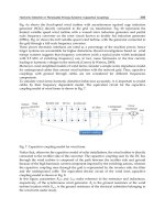
Fig.17-21 show the recorded parameters on MV Line, in the first stage of the heating. In the
recording period (11:20-12:18), the furnace charge was ferromagnetic.


Fig. 17. RMS values of the phase voltages in the cold state (MV Line)
RMS values of phase voltages in the cold state indicate a small unbalance of the load. THD
of phase voltages are within compatibility limits in the first stage of the heating process.
The RMS values of line currents show a poor balance between the phases. The Steinmetz
circuit is not efficient for load balancing in this stage of the melting process.
THD of line currents have values of 20% 70%, and exceed very much the compatibility
limits during the recording period. This indicates a significant harmonic pollution with a
risk of temperature rise.


Fig. 18. THD of phase voltages in the cold state (MV Line)

Power Quality Harmonics Analysis and Real Measurements Data

252

Fig. 19. RMS values of the currents in the cold state (MV Line)


Fig. 20. THD of line currents in the cold state (MV Line)


Fig. 21. DPF and PF per phase 1 in the cold state (MV Line)
In the recorded period of the cold state, power factor (PF) per phase 1 and displacement
factor (DPF) per phase 1 are less than unity; in the time period 12:00 - 12:18 PF is less than

neutral value (0.92). PF is smaller than DPF because PF includes fundamental reactive
power and harmonic power, while DPF only includes the fundamental reactive power
caused by a phase shift between voltage and fundamental current.

Power Quality Problems Generated by Line Frequency Coreless Induction Furnaces

253
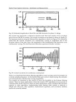
Fig.22-29 show the recorded parameters in the intermediate state of the heating. The furnace
charge was partially melted in the recording period, 13:20-14:18.



Fig. 22. RMS values of phase voltages in the intermediate state (MV Line)


Fig. 23. THD of phase voltages in the intermediate state (MV Line)
In the intermediate state, THD of phase voltages do not exceed the compatibility limits, but
are bigger comparatively with the cold state.



Fig. 24. RMS values of line currents in the intermediate state (MV Line)

Power Quality Harmonics Analysis and Real Measurements Data

254

Fig. 25. THD of line currents in the intermediate state (MV Line)
In the intermediate state, the RMS values of the line currents show a poor balance between
the phases. THD of line currents are remarkably high and exceed the compatibility limits.

Fig. 26. DPF and PF per phase 1 in the intermediate state (MV Line)
The difference between the power factor and the displacement factor is significant in the
intermediate state. This indicates the significant harmonic pollution and reactive power
consumption.
PF per phase 1 is less than neutral value (0.92) almost all the time during the intermediate
state. In the time period 13:20-13:35, PF is very small.


Fig. 27. Active power per phase 1 in the intermediate state (MV Line)

Power Quality Problems Generated by Line Frequency Coreless Induction Furnaces

255

Fig. 28. Reactive power per phase 1 in the intermediate state (MV Line)
In the time period 13:20 - 13:35, the values of reactive power per phase 1 are almost equal to
the values of active power. As a result, the power factor per phase 1 is very poor in the time
period 13:20 - 13:35 (fig.26).


Fig. 29. Apparent power per phase 1 in the intermediate state (MV Line)
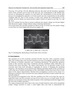
Fig.30-37 show the recorded parameters in the last stage of the heating. The furnace charge
was totally melted in the recording period, 18:02-18:12.


Fig. 30. RMS values of phase voltages in the last stage of the melting process (MV Line)
In the last stage of the melting process, THD of phase voltages are within compatibility
limits, being smaller comparatively with the cold state or the intermediate state.

Power Quality Harmonics Analysis and Real Measurements Data

256

Fig. 31. THD of phase voltages in the last stage of the melting process (MV Line)


Fig. 32. RMS values of line currents in the last stage of the melting process (MV Line)


Fig. 33. THD of line currents in the last stage of the melting process (MV Line)
At the end of the melting process, the RMS values of line currents are much closer
comparatively with cold state or intermediate state. THD of line currents exceed the
compatibility limits, being of 20%…50% during this recording period.
The difference between the power factor and the displacement factor is small in the last stage
of the melting process (fig.34). This indicates a decrease of harmonic disturbances and reactive
power consumption (fig.36), comparatively with the cold state or the intermediate state.

Power Quality Problems Generated by Line Frequency Coreless Induction Furnaces

257
In the time period 18:07 - 18:12, the values of reactive power per phase 1 increase;
consequently, the power factor and the displacement factor per phase 1 decrease.
Recorded values of active power per phase 1 are close to the apparent power values.




Fig. 34. DPF and PF per phase 1 in the last stage of the melting process (MV Line)

Fig. 35. Active power per phase 1 in the last stage of the melting process (MV Line)



Fig. 36. Reactive power per phase 1 in the last stage of the melting process (MV Line)

Power Quality Harmonics Analysis and Real Measurements Data

258

Fig. 37. Apparent power per phase 1 in the last stage of the melting process (MV Line)
6. Conclusion
The measurements results show that the operation of the analyzed furnace determines
interharmonics and harmonics in the phase voltages and harmonics in the currents absorbed
from the network.
THD of phase voltages are within compatibility limits, but voltage interharmonics exceed
the compatibility limits in all the analyzed situations.
THD of line currents exceed the compatibility limits in all the heating stages. Because I
THD

exceed 30%, which indicates a significant harmonic distortion, the probable malfunction of
system components would be very high.
THD of line currents are bigger in intermediate state comparatively with the cold state, or
comparatively with the end of melting. This situation can be explained by the complex and
strongly coupled phenomena (eddy currents, heat transfer, phase transitions) that occur in
the intermediate state.
Harmonics can be generated by the interaction of magnetic field (caused by the inductor)

and the circulating currents in the furnace charge.
Because the furnace transformer is in / connection, the levels of the triple-N harmonics
currents are much smaller on MV Line versus LV Line. These harmonics circulate in the
winding of transformer and do not propagate onto the MV network.
On MV Line, 5
th
and 25
th
harmonics currents exceed the compatibility limits. The levels of
these harmonics are higher on MV Line versus LV Line. Also, THD of line currents and
THD of phase voltages are higher on MV Line versus LV Line, in all the analyzed situations.
The harmonic components cause increased eddy current losses in furnace transformer,
because the losses are proportional to the square of the frequency. These losses can lead to
early failure due to overheating and hot spots in the winding.
Shorter transformer lifetime can be very expensive. Equipment such as transformers is
usually expected to last for 30 or 40 years and having to replace it in 7 to 10 years can have
serious financial consequences.
To reduce the heating effects of harmonic currents created by the operation of analyzed
furnace it must replaced the furnace transformer by a transformer with K-factor of an equal
or higher value than 4.
Peak factors of line currents are high during the heating stages, and characterizes high transient
overcurrents which, when detected by protection devices, can cause nuisance tripping.

Power Quality Problems Generated by Line Frequency Coreless Induction Furnaces

259
The capacitors for power factor correction and the ones from Steinmetz circuit amplify in
fact the harmonic problems.
PF is less than unity in all the analyzed situations. But, Steinmetz circuit is efficient only for
unity PF, under sinusoidal conditions.

Under nonsinusoidal conditions, any attempt to achieve unity PF does not result in harmonic-
free current. Similarly, compensation for current harmonics does not yield unity PF.
For optimizing the operation of analyzed induction furnace, it’s imposing the simultaneous
adoption of three technical measures: harmonics filtering, reactive power compensation and
load balancing. That is the reason to introduce harmonic filters in the primary of furnace
transformer to solve the power interface problems. In order to eliminate the unbalance, it is
necessary to add another load balancing system in the connection point of the furnace to the
power supply network.
7. References
Arrillaga, J., Watson, N. R., & Chen, S. (2000). Power System Quality Assessment, John Wiley
and Sons, ISBN 978-0-471-98865-6, New York.
Ching-Tzong Su, Chen-Yi Lin, & Ji-Jen Wong (2008). Optimal Size and Location of
Capacitors Placed on a Distribution System. WSEAS Transactions on Power Systems,
Vol. 3, Issue 4, (april 2008), pp. 247-256, ISSN 1790-5060.
George, S., & Agarwal, V. (2008). Optimum Control of Selective and Total Harmonic
Distortion in Current and Voltage Under Nonsinusoidal Conditions, IEEE
Transactions on Power Delivery, Vol.23, Issue 2, (april 2008), pp. 937-944, ISSN 0885-
8977.
De la Rosa, F. C. (2006). Harmonics and Power Systems, CRC Press, Taylor&Francis Group,
ISBN 0-8493-30-16-5, New York.
Iagăr, A., Popa, G. N., & Sora I. (2009). Analysis of Electromagnetic Pollution Produced by
Line Frequency Coreless Induction Furnaces, WSEAS TRANSACTIONS on
SYSTEMS, Vol. 8, Issue 1, (january 2009), pp. 1-11, ISSN 1109-2777.
Lattarulo, F. (Ed(s).). (2007). Electromagnetic Compatibility in Power System, Elsevier
Science&Technology Books, ISBN 978-0-08-045261-6.
Muzi, F. (2008). Real-time Voltage Control to Improve Automation and Quality in Power
Distribution, WSEAS Transactions on Circuit and Systems, Vol. 7, Issue 4, (april 2008),
pp. 173-183, ISSN 1109-2734.
Nuns, J., Foch, H., Metz, M. & Yang, X. (1993). Radiated and Conducted Interferences in
Induction Heating Equipment: Characteristics and Remedies, Proceedings of Fifth

European Conference on Power Electronics and Applications, Brighton, UK., Vol. 7, pp.
194-199, september 1993.
Panoiu, M., Panoiu, C., Osaci, M. & Muscalagiu, I. (2008). Simulation Result about
Harmonics Filtering Using Measurement of Some Electrical Items in Electrical
Installation on UHP EAF, WSEAS Transactions on Circuit and Systems, Vol. 7, Issue 1,
(january 2008), pp. 22-31, ISSN 1109-2734.
Rudnev, V., Loveless, D., Cook, R., & Black, M. (2002). Handbook of Induction Heating, CRC
Press, Taylor&Francis Group, ISBN 0824708482, New York.
Sekara, T. B., Mikulovic, J.C., & Djurisic, Z.R. (2008). Optimal Reactive Compensators in
Power Systems Under Asymmetrical and Nonsinusoidal Conditions, IEEE

Power Quality Harmonics Analysis and Real Measurements Data

260
Transactions on Power Delivery, Vol. 23, Issue 2, (april 2008), pp. 974-984, ISSN 0885-
8977.
CA8334, Three Phase Power Quality Analyser, technical handbook, Chauvin Arnoux,
France, 2007.
IEC 61000-3-4, EMC, Part 3-4: Limits – Limitation of Emission of Harmonic Currents in Low-
Voltage Power Supply Systems for Equipment with Rated Current Greater than
16A, 1998.
IEC/TR 61000-3-6, EMC, Part 3-6: Limits – Assessment of Harmonic Emission Limits for the
Connection of Distorting Installations to MV, HV and EHV Power Systems
(revision), 2005.
Power Quality for Induction Melting in Metal Production, TechCommentary Electric Power
Research Institute (EPRI), U.S.A., 1999, available at:

11
Harmonic Distortion in Renewable
Energy Systems: Capacitive Couplings

Miguel García-Gracia, Nabil El Halabi,
Adrián Alonso and M.Paz Comech
CIRCE (Centre of Research for Energy Resources and Consumption)
University of Zaragoza
Spain
1. Introduction
Renewable energy systems such as wind farms and solar photovoltaic (PV) installations are
being considered as a promising generation sources to cover the continuous augment
demand of energy.
With the incoming high penetration of distributed generation (DG), both electric utilities
and end users of electric power are becoming increasingly concerned about the quality of
electric network (Dugan et al., 2002). This latter issue is an umbrella concept for a multitude
of individual types of power system disturbances. A particular issue that falls under this
umbrella is the capacitive coupling with grounding systems, which become significant
because of the high-frequency current imposed by power converters.
The major reasons for being concerned about capacitive couplings are:
a. Increase the harmonics and, thus, power (converters) losses in both utility and customer
equipment.
b. Ground capacitive currents may cause malfunctioning of sensitive load and control
devices.
c. The circulation of capacitive currents through power equipments can provoke a
reduction of their lifetime and limits the power capability.
d. Ground potential rise due to capacitive ground currents can represent unsafe
conditions for working along the installation or electric network.
e. Electromagnetic interference in communication systems and metering infrastructure.
For these reasons, it has been noticed the importance of modelling renewable energy
installations considering capacitive coupling with the grounding system and thereby
accurately simulate the DC and AC components of the current waveform measured in the
electric network.
Introducing DG systems in modern distribution networks may magnify the problem of

ground capacitive couplings. This is because DG is interfaced with the electric network via
power electronic devices such as inverters.
These capacitive couplings are part of the electric circuit consisting of the wind generator,
PV arrays, AC filter elements and the grid impedance, and its effect is being appreciated in
most large scale DG plants along the electric network (García-Gracia et al., 2010).

Power Quality Harmonics Analysis and Real Measurements Data

262
Power electronic devices, as used for DG, might be able to cause harmonics. The magnitude
and the order of harmonic currents injected by DC/AC converters depend on the technology
of the converter and mode of its operation (IEC Std. 61000-4-7, 2010, IEEE Std. 519-1992, 1992).
Due to capacitive coupling between the installation and earth, potential differences imposed
by switching actions of the converter inject a capacitive ground current which can cause
significant electromagnetic interferences, grid current distortion, losses in the system, high-
noise level in the installation and unsafe work conditions (Chicco et al., 2009).
Several renewable system installations analyses have been reported (Bellini, 2009, Conroy,
2009, Luna, 2011, Sukamonkol, 2002, Villalva, 2009), where most theoretical analysis and
experimental verifications have been performed for small-scale installations without
considering capacitive coupling. Power electronics models and topologies also have been
studied, but without considering the amount of losses produced by the capacitive current that
appears due to the switching actions (Zhow, 2010, Chayawatto, 2009, Kim, 2009). In (Iliceto &
Vigotti, 1998), the total conversion losses of a real 3 MW PV installation have been studied
considering reflection losses, low radiation and shadow losses, temperature losses, auxiliary
losses, array losses and converters losses. The latter two factors sum a total of 10% of the rated
power where part of these losses is due to the capacitive coupling that was neglected.
Therefore, for an accurate study of power quality, it is important to model DG installations
detailing the capacitive coupling of the electric circuit with the grounding system, which are
detailed for PV installations and wind farms in Sections 2 and 3, respectively. These models
allow analyzing the current distortion, ground losses and Ground Potential Rise (GPR) due

to the capacitive coupling. The combined effect of several distributed generation sources
connected to the same electric network has been simulated, and results have been presented
together with solutions based on the proposed model to minimize the capacitive ground
current for meeting typical power quality regulations concerning to the harmonic distortion
and safety conditions.
2. Capacitive coupling in solar-photovoltaic installation
The region between PV modules and PV structure essentially acts as an insulator between
layers of PV charge and ground. Most shunt capacitive effects that may be ignored at very
low frequencies can not be neglected at high frequencies for which the reactance will
become relatively small due to the inverse proportionality with frequency f and, therefore, a
low impedance path is introduced between power elements and ground.
This effect is present in PV installations because of the high frequency switching carried out
by the converters stage, which arises different capacitive coupling between modules and
ground. Thus, the capacitive effect must be represented as a leakage loop between PV
arrays, cables and electronic devices and the grounding system. By means of this leakage
loop, capacitive currents are injected into the grounding system creating a GPR along the PV
installation which introduces current distortion, electromagnetic interference, noise and
unsafe work conditions. For this reason, an accurate model of these capacitive couplings are
requiered for PV installations.
2.1 Equivalent electric circuit for ground current analysis
Depending on the switching frequency, the harmonics produced may be significant
according to the capacitive coupling and the resonant frequency inside the PV installation.

Harmonic Distortion in Renewable Energy Systems: Capacitive Couplings

263
Moreover, every PV array is considered as an independent current source with a DC current
ripple independent of the converter ripple. These ripple currents are not in synchronism
with the converter and produce subharmonics in the DC circuit which increase the Total
Harmonic Distortion in the current waveform (THDI) (Zhow et al., 2010).

The typical maximum harmonic order h = 40, defined in the power quality standards,
corresponds to a maximum frequency of 2 kHz (with 50 Hz as fundamental frequency) (IEC
Std. 61000-4-7, 2002). However, the typical switching frequency of DC/DC and DC/AC
converters, usually operated with the Pulse Width Modulation (PWM) technique, is higher
than 3 kHz. Hence, higher order harmonics up to the 100th order, can be an important
concern in large scale PV installations where converters with voltage notching, high pulse
numbers, or PWM controls result in induced noise interference, current distortion, and local
GPR at PV arrays (Chicco et al., 2009).
A suitable model of capacitive couplings allows reproducing these harmonic currents
injected not only into the grid, but also into the DC circuit of the PV installation that would
lead to internal resonant, current distortion and unsafe work conditions where capacitive
discharge currents could exceed the threshold of safety values of work (IEEE Std. 80-2000,
2000). The capacitive coupling is part of the electric circuit consisting of the PV cells, cables
capacitive couplings, AC filter elements and the grid impedance, as shown in Fig. 1, and its
effect is being appreciated in most large scale PV plants.





Fig. 1. Model of PV module, PV array and capacitive coupling with PV structure.

Power Quality Harmonics Analysis and Real Measurements Data

264
2.2 Behavior of the PV installation considering capacitive coupling
Normally, numerous PV modules are connected in series on a panel to form a PV array as it
is shown in Fig. 1. The circuit model of the PV module (Kim et al., 2009) is composed of an
ideal current source, a diode connected in parallel with the current source and a series
resistor. The output current of each PV module is determined as follows:

·
·exp
·
s
sc d sc o
T
VIR
II I I I
nV













(1)
where I
o
is the diode saturation current, V the terminal voltage of a module, n the ideal
constant of diode, V
T
is the thermal potential of a module and it is given by m·(kT/q) where

k the Boltzmann's constant (1.38E-23 J/K), T the cell temperature measured in K, q the
Coulomb constant (1.6E-19 C), and m the number of cells in series in a module. I
sc
is the
short circuit current of a module under a given solar irradiance. I
d
is the diode current,
which can be given by the classical diode current expression. The series resistance R
s

represents the intrinsic resistance to the current flow.
The capacitive coupling of PV modules with the ground is modelled as a parallel resistance
R
pv
and capacitor C
pv
arrangement which simulates the frequency dependency on the
insulator between PV modules and the grounding system. The PV structure is connected to
the grounding system represented in the model by the grounding resistance R
g
.
Taking into account that the converter represents a current source for both DC circuit and
AC circuit of the PV installation, an equivalent circuit is deduced to analyze the capacitive
coupling effect over the current and voltage waveforms.
The equivalent circuit of both DC circuit of the PV installation and AC circuit for connection
to the grid as seen between inverter terminals and ground is illustrated Fig. 2. In the AC
circuit R
ac_cable
, L
ac_cable

and C
ac_cable
are the resistance, inductance and capacitance of the AC
underground cables, R
g_es
is the ground resistance at the substation and L
filter
and C
filter
are
the parameters of the LC filter connected at AC terminals of the inverter.


Fig. 2. Capacitive coupling model for the DC and AC electric circuit of a PV installation.
The inclusion of R
pv
and C
pv
on the PV equivalent circuit allows representing the leakage
path for high frequency components between PV modules and ground. This DC equivalent
circuit is represented by the following continuous-time equations, at nominal operating
condition

1
12
d() 1 1
·() ·() ·()
d
c
in

ccc
R
it
vt it vt
tL L L

(2)

2
122
d() 1 1 1
·() ·() · ()
d·() ·()· ··()
c s g c s g pv pv pv pv s g
it
it it vt
tCRR CRRCR CRRR




 



(3)

Harmonic Distortion in Renewable Energy Systems: Capacitive Couplings

265

2
12
d() 1 1
· () · ()
d
cc
vt
it it
tC C
 (4)

12
2
d() ·
·() ·()
d·() · ·()·
1
·() · ()
··( ) ·
pv g pv g g g
c s g pv pv c s g pv pv
g
pv
pv pv s g pv pv
vt R R R R R
it it
tCRR CRCRRCR
R
vt v t

CR R R CR











(5)
According to the equivalent DC circuit shown in Fig. 2, i
1
(t) and i
2
(t) are the current of mesh
1 and mesh 2, respectively, v
in
(t) is the injected voltage by the converter, v
2
(t) the voltage at
node 2 and v
pv
(t) is the voltage between PV module and ground and represents the
parameter under study. Parameter C
c
represents the capacitive coupling between cables and
ground and R

c
and L
c
are the resistance and inductance of the cable, respectively.
In some simplified models of PV installation (Villalva, 2009, Kim, 2009, Bellini, 2009), the
capacitance C
pv
and resistance R
pv
are considered like infinite and zero, respectively. Then,
the capacitive coupling with the grounding system is totally neglected. Even ground
resistance of the PV installation is not considered (R
g
= 0).
The PV arrays are connected to a DC system of 700 V, and the power is delivered to an
inverter stage based on four inverters of 125 kW in full bridge topology and operation
frequency of 3.70 kHz. The underground cables, which connect the PV arrays to the inverter
stage, have been included through their frequency dependent model.
The electrical parameters of the capacitive coupling between PV arrays and grounding
system are shown in Table 1 and have been adjusted according to the field measurement in
order to simulate the response of the capacitive coupling model accurately against the
harmonics injected by the operation of the converters.

Element Parameter Value
PV array
Operation voltage 700 Vdc
Capacitance C
PV
1x10
-9

F
Resistance R
PV
1x10
7

Series Resistance R
S

0.30

DC cable
Resistance R
C
0.25 /km
Inductance L
C
0.00015 H/km
Capacitive coupling C
C
1x10
-4
F/km
Filter LC
Inductance L
filter
90 µH
Capacitance C
filter
0.756 mF

Underground cable
Positive sequence impedance
0.3027 + j 0.1689
/km
Zero sequence impedance
0.4503 + j 0.019
/km
Zero sequence susceptance 0.1596 mS/km
Power grid
Thevenin voltage 20 kV
Thevenin impedance
0.6018+j 2.4156

Ground resistance R
g
1.2 
Table 1. Electric parameters for the solar PV installation capacitive grounding model.

Power Quality Harmonics Analysis and Real Measurements Data

266
The frequency response of both capacitive coupling and simplified model for the DC circuit of
a PV installation operating at nominal operating condition is shown in the Bode diagram of
Fig. 3. The capacitive coupling model presents a considerable gain for waveforms under 108
kHz in comparison with the simplified model which has a limited gain for this range of
frequencies. Hence, the capacitive coupling model is able to simulate the leakage loop between
PV module and grounding system for high frequencies, unlike the simplified model.


Fig. 3. Bode diagram for both capacitive coupling model (solid line) and simplified model

(dashed line) for the DC circuit of a PV installation.
The PV installation modelled consists of 184 PV arrays connected in parallel to generate
1 MW. Both circuits have been modelled to analyze the mutual effect raised from the
capacitive couplings between the electric circuits and the grounding system, at rated
operating conditions. The simulation has been performed using PSCAD/EMTDC [PSCAD,
2006] with a sampling time of at least 20 µs.
The current and voltage waveforms obtained from the proposed model together with the
FFT analysis are shown in Fig. 4a and Fig. 4b. The THDI and THDV obtained from
simulations are 26.99% and 3725.17%, respectively, where the DC fundamental
component of current is 88.56 mA, and the fundamental voltage component is 8.59 V. The
frequencies where most considerable harmonic magnitudes are the same of those
obtained at field measurement; 3.70 kHz, 11.10 kHz, 14.80 kHz and 18.50 kHz within a
percentage error of ±27.42% for fundamental component and ±15.35% for the rest of
harmonic components.
2.3 Additional information provided by the PV installation capacitive coupling
The model considering capacitive coupling between PV modules and grounding system of
the installation leads to an accurate approximation to the response of the PV installation
against the frequency spectrum imposed by the switching action of the inverters. This
approximation is not feasible using simplified models because of the bandwidth limitation
shown in Fig. 3 for high frequencies.

Harmonic Distortion in Renewable Energy Systems: Capacitive Couplings

267

(a)


(b)
Fig. 4. Simulation result of the capacitive coupling model: (a) voltage waveform between PV

array and grounding system and (b) FFT analysis of the voltage waveform obtained.
Simulation results indicate that ground current in large scale PV installations can be
considerable according to the values expressed in (IEEE Std. 80-2000, 2000). In the range of
9-25 mA range, currents may be painful at 50-60 Hz, but at 3-10 kHz are negligible (IEC
60479-2, 1987). Thus, the model allows the detection of capacitive discharge currents that
exceeds the threshold of safety values at work.
Because of large scale installations are systems with long cables, the resonant frequency
becomes an important factor to consider when designing the AC filters and converters
operation frequency. The proposed model accurately detects the expected resonant
frequency of the PV installations at 12.0 kHz with an impedance magnitude Z of 323.33

while simplified models determine a less severe resonant at a frequency value of 15.50 kHz
with a Z of 150.45
, as shown in Fig. 5.
This latter resonant frequency is misleading and pointless for the real operating parameters
of the installation. The total DC/AC conversion losses obtained from simulations is 5.6%
when operating at rated power, which is equivalent to 56.00 kW. Through the proposed
model, it has been detected that a 22.32% of the losses due to the DC/AC conversion is

Power Quality Harmonics Analysis and Real Measurements Data

268
because of the capacitive coupling modelled. Thus, a 1 MW PV installation as modelled in
Fig. 2 presents 12.50 kW of losses due to the capacitive couplings or leakage loop between
PV modules and ground.



Impedance |Z| ()
Frequency (Hz)

Fig. 5. Resonance frequency of the PV installation without capacitive coupling (dashed line)
and considering capacitive couplings (solid line).
3. Capacitive coupling in wind farms
Wind energy systems may contribute to the distribution network voltage distortion because
of its rotating machine characteristics and the design of its power electronic interface. As
presented in Fig. 6, wind energy system designs incorporate a wide range of power
electronic interfaces with different ratings (Comech et al., 2010).



Fig. 6. Wind turbine configurations.
(
b
)
GB

(a)
GB
GB
(c)