Fundamental and Advanced Topics in Wind Power Part 4 pptx

Verification of Lightning Protection Measures

79
8
0m
3000m
1000m

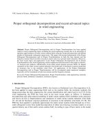
Fig. 11. A typical model of a turbine used in the research. The size of the analysis volume is
considerably larger than the turbine, in this case 1km x 1km x 3km.
fulfilling the inception conditions divided by the height of the analysis volume, whereas the
term successful upward leader refers to a leader that will propagate upwards self
consistently.
Having the stabilisation field defined for each point on the structure, the second part of the
process is to follow the procedure for assigning static leader inception zones, finally
resulting in individual probabilities as seen above. To understand the basis of the discrete
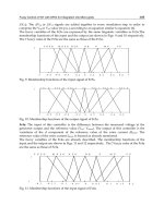
probabilities, 3D scatter plots of the successful leader inception points for the orientation 30°
to horizontal level are shown in Fig. 12. Here it is clear how the upward leader inceptions
occur with a larger distance to the downward leader tip for higher prospective peak
currents (Left), whereas lower prospective peak currents allow the downward leader to
approach closer to the turbine before upward leader inception (Right).

-500
0
500
-600
-400
-200
0
200

400
600
-550
-500
-450
-400
-350
-300
-250
-200
-150
-100
-50
0
Z-coordinates [ m]
Y-coordi nates [ m]
Scat ter plot of leader incept ion points , 30deg, 40kA
X-coordinate, negative heights [m ]

-500
0
500
-600
-400
-200
0
200
400
600
-550

-500
-450
-400
-350
-300
-250
-200
-150
-100
-50
0
Z-coordinates [m]
Scatter plot of leader inception points, 30deg, 20kA
Y-c oordina tes [m ]
X-coordinat e, negativ e heights [m]

Fig. 12. Scatter plots showing origins of the downward leaders, leading to successful
upward leader inception. Each colour corresponds to different attachment points. Left:
40kA, Right 20kA.
By evaluating the results presented graphically on Fig. 12 for three different rotor
orientations and the four different peak current levels, an indication of the attachment point
distribution for all possible situations is derived. In practice, it is done by counting the
number of points with each individual colour and relating them to the total number of
points (corresponding to the static leader inception zone defined previously). On Fig. 13,
examples of the results considering two different rotor orientations and the 18 different
points incepting lightning strikes are shown.

Fundamental and Advanced Topics in Wind Power

80

A
B
C
D
E
K
M
L
J
I
H
G
F
R
P
Q
O
N
A
B
C
D
E
K
M
L
J
I
H
G

F
R
P
Q
O
N

30° - Probabilities [%] 60° - Probabilities [%]
Point 60kA 40kA 20kA 10kA Point 60kA 40kA 20kA 10kA
A 50 50 50 50 A 100 100 99 98
F 50 50 50 50 F 0 0 1 2
Fig. 13. Attachment point distribution along five points for each blade, two points on the
rear of the nacelle and the tip of the spinner.
In Fig 13. it is seen how the blade tips are the only exposed structures to peak currents down
to 10kA and that the attachment distribution dictates equal probability for each of the
upward pointing blades in the 30° orientation. For the second orientation (60° with
horizontal), the probability of striking the upward pointing blade is by far larger than the
probability of striking other parts of the turbine. However, as indicated in Fig. 13, the
probability of striking the blade tip on the horizontal blade (point F) increases as the peak
current is lowered.
Intuitively, the general conclusion based on the probabilities found above seems too simple.
However, they depend strictly on the geometry and the algorithms derived. By
investigating the situation having the rotor in the 30° orientation, the differences at the
different peak return stroke currents are clarified. Fig. 14 shows three views of the turbine
along with the points representing the leader tip positions at the successful inception of the
upward leader. The blue points correspond to the situation where point A incepts upward
leaders, whereas the green points represent the situations where point F receives the
lightning strike.

Fig. 14. Scatter plots visualising the 30° orientation considering 10kA prospective peak
currents.

Verification of Lightning Protection Measures

81
On Fig. 15 two plots of the same data are shown with a view parallel to the rotor axis and
from directly above the turbine. In each case it is seen how the sphere caps drawn by the
coloured points tend to wrap the turbine more smoothly at such low peak currents, so that
the turbine geometry becomes more apparent to the leader tip. At high peak currents only
the turbine extremities are exposed, whereas for low peak currents suddenly the less
exposed structures on the turbine might incept lightning strikes.


Fig. 15. Scatter plots shown parallel to the rotor axis (left) and from directly above the
turbine (right), 10kA prospective peak current.
If full simulations were to be conducted at even smaller peak currents, the tendency would
be that suddenly inboard receptors or the rear of the nacelle would be exposed enough to
incept direct lightning strikes. However, at such low peak currents the associated damages
are easier to control by suitable protection measures.
To prove this tendency, a simple situation is simulated manually by a vertical leader
approaching directly above the turbine. Fig. 16 shows the leader tip height at connecting
leader inception as well as the points from which the inception occurs for different peak
currents. When lowering the current, the height of inception is lowered as well, meaning
that the leader tip gets closer to the turbine before anything happens. Down to 8.5kA, the
blade tip still incepts the connecting leaders first (A and F). At 8.25kA and 8kA, the fifth
receptor pair (E and J) tends to incept leaders initially. The blade tips are not struck in this
case. Lowering the current even further down to 7kA results in the exposure of the rear of
the nacelle, since points K and L now incepts the initial leaders.

Fig. 16. By lowering the prospective peak return stroke current, attachment points elsewhere
than the blade tips becomes possible.

Fundamental and Advanced Topics in Wind Power

82
Considering higher peak currents than the 60kA used in these simulations, the attachment
distribution would be similar, as shown in the 60kA simulations, since the sphere caps will
move further away from the turbine. The findings using vertical leaders therefore shows
that inboard parts of the structure are only exposed to small amplitude lightning strikes,
and that lightning strikes having peak amplitudes in excess of 10kA will attach to the blade
tips.
3.1.4 Application of attachment point modelling
Modelling of the lightning attachment points on wind turbines is used to foresee where and
with which amplitudes the lightning discharge will affect the structure. This enables the
lightning protection engineer to place adequate protection measures at the right locations
without over-engineering the solutions. To get the turbine designs certified by DNV, GL or
similar, it requires that the protection principles applied are verified according to IEC 61400-
24. Here either testing or modelling becomes necessary.
In the larger perspective, numerical modelling has also been used to address the issues of
subdividing the wind turbine blades into lightning protection zones. The principle is known
from the avionics industry, were the areas of an aircraft fuselage or a wing is divided into
zones struck directly, experiencing a swept stroke, hang on zones and similar (SAE ARP
5414). The reason for considering zoning as an important part of the lightning protection
design is that damages and attachment points inboard the blade tips - foreseen by the
general EGM methods - are not experienced. Data from recent field surveys on modern
wind turbines indicate that mainly attachments at the blade tips occur (Madsen et al. 2010).

11,9%

88,1%
0,0%
20,0%
40,0%
60,0%
80,0%
100,0%
0 5 10 15 20 25 30 35 38,8
Attachnment point distribution
Length of blade [m]

9,7%
27,6%
40,5%
0,0%
20,0%
40,0%
60,0%
80,0%
100,0%
Attachnment point distribution
Length of blade [m]

Fig. 17. Left: Attachment point distribution on 236 blades (39m) after two years of lightning
exposure at the 'Horns Rev' wind farm, Right: Attachment point distribution of 2818
identified lightning attachment points on 45m blades.
From both graphs on Fig. 17 it is obvious how the blade tips are most favoured when it
comes to lightning attachment. The main conclusion from the recent site inspection program
is that the tip of the blades (within 1.5m) receives 70% of the lightning strikes, that 90% of
the lightning strikes attaches within the outermost 6m of the blade, and that the remaining

10% attaches further inboard (6m from the tip). No correlations have been done so far
considering the size of the erosion on receptors, and hence the current peak amplitude /
specific energy / charge levels, but these are topics that will be addressed by the research
team in future publications.
Based on the field surveys, and heavily supported by the numerical computations, it was
therefore decided to define a zoning concept of wind turbine blades according to Fig. 18.

Verification of Lightning Protection Measures

83


Fig. 18. New zoning concept based on the expected peak current amplitudes. (Madsen et al.
2010)
The zoning concept is regarded a possible upgrade for the test requirements in the next
revision of the IEC 61400-24.
3.2 Modelling of magnetic fields
When a DC current is injected through a complex structure with several different paths, the
current will be distributed according to the resistances of the different paths. There are no
mutual couplings of neither inductive nor capacitive nature, since the currents or voltages
are not time dependant. The solution of the current distribution is then straightforward, and
can be performed using simple linear algebra.
If AC currents or transient currents are injected, the dI/dt of the AC current or the dU/dt of
the AC voltage will introduce mutual couplings, which means that the current flowing in
one conductor might induce a voltage on another conductor, or vice versa. In this case, the
mutual couplings must be identified. It can be done analytically on very simple structures
(two parallel wires, two wires of infinite length crossing at a fixed angle, etc.), but when it
comes to real physical structures, numerical methods are required.
The numerical codes typically used are based on the FDTD (Finite Difference Time Domain)
or the FEM (Finite Element Method). In both cases, the structure geometry is subdivided

into a finite number of elements, and Maxwell Equations are then solved for each element
respecting the mutual boundary conditions.
3.2.1 Current components
To model voltage drops during the interception of a lightning strike, the different
components of the lightning strike must be considered individually. In the international
standards for lightning protection, three characteristic current components for a Level 1
stroke are derived:
- The first return stroke, a 200kA current pulse with a rise time of 10µs and a decay time
of 350µs. In the frequency domain, this waveform is simulated by an oscillating
waveform exhibiting a frequency of 25kHz.
- The subsequent return stroke, a 50kA current pulse with a rise time of 0.25µs and a
decay time of 100µs. In the frequency domain, this waveform is simulated by an
oscillating waveform exhibiting a peak frequency of 1MHz.
- The continuing current, a DC current pulse of amplitude 200-800A and duration of up
to a second.

Fundamental and Advanced Topics in Wind Power

84
In natural lightning, all possible combinations occur, but for verification of lightning
protection systems (simulation and testing) these three individual components apply. In the
case of determining the maximum magnetic fields within the nacelle, the first and the
subsequent return stroke are of most concern.
Due to the frequencies of the lightning current and the permeability of the involved
conductor materials for the nacelle structure, the skin effect becomes very important.
Considering Iron with a relative permeability of 200 and conductivity in the range of 10
7

S/m, the skin depth for a 10kHz current component will be only 0.11mm, decreasing with
increasing frequency. Therefore, the high frequency model (>10kHz) treats the solid

structure of the nacelle as thin boundaries, since it can be assumed that all current flows at
the structure extremity.
3.2.3 Modelling output
The simulations consider several different attachment points for the lightning strike, by
injecting the lightning current into different places at the nacelle. A typical model of a wind
turbine considering magnetic fields and current distribution when a blade is struck is seen
on Fig. 19.


Fig. 19. The configuration where the turbine is struck on a blade pointing to the left with an
angle of 45° with horizontal. The line extending from the HUB is simulating the blade down
conductor.
In the case of a lightning strike to a blade located on the left side of the nacelle, the
magnitude of the magnetic field during the first return stroke (200kA@25kHz) is illustrated
on Fig. 20.
The magnetic field is visualized by drawing surfaces of equal magnitude. The red surface
represents an area where the magnetic field attains a value of 30kA/m, the green surface
represents a value of 20kA/m, the light blue surface represents a value of 10kA/m and the
dark blue a value of 5kA/m.
The magnitude and distribution of the magnetic field around the geometry depends on the
current path and current density on the surface of the structure. By evaluating the field
distribution on Fig. 20, it is seen that the highest field strengths are obtained close to the
main current paths where these are of limited size (the down conductor, lightning channel,
etc.). At the rear of the nacelle and around the structural bars some metres away from the

Verification of Lightning Protection Measures

85
HUB, the field is much lower. The current flowing in the nacelle construction works as the
current in a faraday cage; hence the magnetic field in the centre of the nacelle is cancelled

out to some degree.




Fig. 20. Illustration of the magnetic field magnitude during a first return stroke represented
by 200kA at 25kHz. The magnetic field is visualized by an iso-surface plot in which red
represents a magnetic field strength of 30 kA/m, green represents 20 kA/m, light blue
represents 10 kA/m and dark blue represents a field strength of 5 kA/m. Magnetic fields
strength above 30 kA/m and below 5 kA/m has been omitted to simplify the illustration.
The current distribution within the different structural components also tends to minimize
the magnetic field in the centre of the nacelle. This is seen more clearly at the following 2D
slice plot, where the magnitude of the magnetic field is plotted for two different slice plots.




Fig. 21. 2D slice plot of the magnetic field when 200kA at 25kHz is conducted from one of
the blades towards the tower base. The range for the plot is 5kA/m (blue) to 30kA/m (red).

Fundamental and Advanced Topics in Wind Power

86
The magnetic field is forced to the outside of the nacelle structure, due to the mutual
coupling between the current flowing in the different structural components. The
consequence is that the structural bars act as a Faraday cage for the interior of the nacelle,
which is to be considered when placing panels and cables within the nacelle.
3.2.4 Application of results
Once the magnetic fields within the structure are known, panels and shielded cables can be
selected to ensure certain compatibility between the control and sensor systems within the

nacelle and the environment in terms of magnetic fields. Based on the current distribution
also obtained by the numerical simulations, expressions can be derived, which couple
lightning currents in the main structure with induced currents in cable shields.
Having the currents flowing on shielded cable or EMC enclosures with well-known transfer
impedance, finally enables the designer to calculate the expected potential rise on
conductors and hence select appropriate surge protection.
Along with testing, it is believed that future verification will benefit considerably by
numerical modelling of lightning protection systems.
4. Conclusion
The present chapter presents general aspects of lightning protection to be considered when
designing lightning protection systems for wind turbines. Since the release of the new
standard IEC 61400-24, for lightning protection of wind turbines, verification of the
protection measures has become mandatory. The verification can be done by either high
voltage or high current testing, or by means of numerical modelling that has previously
been verified against experimental findings or field surveys.
The test programme begins with an Initial Leader Attachment Test, defining where the
turbine or in most cases the blade will most likely be struck. Hopefully, the blade will only
be struck at places designed to handle the lightning current (lightning receptors) otherwise
the design must be improved before passing the blade on to the high current test.
After defining these possible attachment points, the blade is tested in a high current
laboratory to be subjected to the threat of the lightning current. The various lightning
current waveforms are injected into the locations determined by the high voltage test, and
the damage or wearing associated with these tests might require further design
optimisation.
At an early stage of a design phase or in situations where testing is not an option, numerical
modelling can be used as mean of verification. Basically the same two phenomena are
modelled, the attachment process and the current conduction.
Attachment point modelling aims at identifying possible lightning attachment points on the
wind turbine and defines the probabilities that certain areas will receive strikes of certain
amplitudes. The methodology is used to foresee the most optimum placement of air

termination systems on the nacelle and the blades, which is no longer applicable to the EGM
methods according to IEC 61400-24.
Simulation of current distribution and magnetic fields in especially the nacelle structure is
vital for design engineers to require a sufficient degree of shielding for their equipment. The
magnetic environment within or adjacent to the nacelle structure during a lightning strike, is
considerably higher than what the general EMC standards describe.

Verification of Lightning Protection Measures

87
5. Acknowledgement
The research within lightning protection of wind turbines is carried out in a major
community worldwide including representatives from the wind turbine manufacturers,
wind turbine operators, test facilities, universities, public and private research institutes, etc.
The knowledge accumulated within this group of researchers, and published at
international conferences, in scientific journals and at commercial expos would not be
possible without the involvement and professionalism of all participants.
A special acknowledgement is dedicated to friends and colleagues that have helped me and
the wind turbine industry to gain a higher level of engineering expertise within lightning
protection of wind turbines.
6. References
Madsen, S.F. (2006). Interaction between electrical discharges and materials for wind turbine
blades particularly related to lightning protection, Ørsted-DTU, The Technical
University of Denmark, Ph.D. Thesis, ISBN: 87-91184-60-6
Larsen, F.M & Sorensen, T. (2003). New lightning qualification test procedure for large wind
turbine blades, Proceedings of International Conference on Lightning and Static
Electricity, Blackpool, UK.
Madsen, S.F., Holboll, J., Henriksen, M., Bertelsen, K. & Erichsen, H.V. (2006) New test
method for evaluating the lightning protection system on wind turbine blades.
Proceedings of the 28th International Conference on Lightning Protection, Kanazawa,

Japan.
Holboll, J., Madsen, S.F., Henriksen, M., Bertelsen, K. & Erichsen, H.V. (2006) Lightning
discharge phenomena in the tip area of wind turbine blades and their dependency
on material and environmental parameters. Proceedings of the 28th International
Conference on Lightning Protection, Kanazawa, Japan.
Bertelsen, K., Erichsen, H.V. & Madsen, S.F. (2007) New high current test principle for wind
turbine blades simulating the life time impact from lightning discharges.
Proceedings of the 30th International Conference on Lightning and Static Electricity, Paris,
France.
IEC 61400-24 Ed. 1.0. Wind turbines – Part 24: Lightning Protection, 2010.
IEC TR 61400-24. Wind turbine generator systems – Part 24: Lightning protection, 2002.
SAE ARP 5416. Aircraft Lightning Test Methods, Section 5: Direct Effects Test Methods,
2004.
IEC 62305-1 Ed. 1.0. Protection against lightning – Part 1: General principles, January 2006.
EN 50164-1 Lightning Protection Components (LPC) – Part 1: Requirements for connection
components, September 1999.
Heater, J. and Ruei, R. (2003). A Comparison of Electrode Configurations for Simulation of
Damage Caused by a Lightning Strike, Proceedings of International Conference on
Lightning and Static Electricity, Blackpool, UK.
IEC 62305-2 Ed. 1.0, Protection against lightning – Part 2: Risk management, January 2006.
IEC 61000-4-5 Ed. 2.0, Electromagnetic compatibility (EMC) – Part 4-5: Testing and
measurement techniques – Surge immunity test, November 2005.
Madsen, S.F., Bertelsen, K., Krogh, T.H., Erichsen, H.V., Hansen, A.N., Lønbæk, K.B. (2010)
Proposal of new zoning concept considering lightning protection of wind turbine

Fundamental and Advanced Topics in Wind Power

88
blades. Proceedings of the 30th International Conference on Lightning Protection, Calgari,
Italy.

Becerra, M. (2008) On the Attachment of Lightning Flashes to Grounded Structures,
Doctoral thesis, Uppsala University, ISBN :XXXX.
Becerra, M. and Cooray, V. (2005) A simplified model to represent the inception of upward
leaders from grounded structures under the influence of lightning stepped leaders,
Procedings of the 29th International Conference on Lightning and Static Electricity,
Seattle Washington, USA.
Becerra, M., Cooray V. & Abidin H.Z. (2005) Location of the vulnerable points to be struck
by lightning in complex structures, Procedings of the 29th International Conference on
Lightning and Static Electricity, Seattle Washington, USA.
Bertelsen, K., Erichsen, H.V., Skov Jensen M.V.R. & Madsen, S.F. (2007) Application of
numerical models to determine lightning attachment points on wind turbines,
Proceedings of the 30th International Conference on Lightning and Static Electricity, Paris,
France.
Madsen, S.F. & Erichsen, H.V. (2008) Improvements of numerical models to determine
lightning attachment points on wind turbines, Procedings of the 29th International
Conference on Lightning Protection, Uppsala, Sweden.
Cooray, V., Rakov, V. & Theethayi, N. (2004) The relationship between the leader charge
and the return stroke current – Berger’s data revisited, Procedings of the 27th
International Conference on Lightning Protection, Avignon, France.
Madsen, S.F. & Erichsen, H.V. (2009) Numerical model to determine lightning attachment
point distributions on wind turbines according to the revised IEC 61400-24,
Proceedings of the 31st International Conference on Lightning and Static Electricity,
Pittsfield, Massachussetts, USA.
Golde, R.H. (1977) Lightning Conductor, Chapter 17 in Golde, R.H. (Ed.), Lightning, vol. 2,
Academic Press: London, UK.
SAE ARP 5414. Aircraft Lightning Zoning, 1999.
5
Extreme Winds in Kuwait
Including the Effect of Climate Change
S. Neelamani and Layla Al-Awadi

Coastal Management Program, Environment and Life Sciences Centre,
Kuwait Institute for Scientific Research,
Kuwait
1. Introduction
Wind turbines need to convert the kinetic energy of normal wind speed into electric power
but the structure needs to withstand the wind loads exerted by the extreme wind speed on
the mast and blades. Also high rise buildings around the world are designed for a wind
speed whose probability of exceedence is 2% (Gomes and Vickery (1977), Milne (1992),
Kristensen et al., (2000), Sacré (2002) and Miller (2003)). Recently, the State of Kuwait has
approved construction of multistory buildings up to about 70 floors. For safe and optimal
design of these high rise buildings, extreme wind speeds for different return periods and
from different directions are essential. Wind data, measured at 10 m above the ground level
at different locations can be used for the prediction of extreme wind speeds at that elevation.
These unexpected high wind speed from different directions dictates the design of many
structures like towers, high rise buildings, power transmission lines, devises for controlling
the sand movements in desert areas, ship anchoring systems in ports and harbors, wind
power plants on land and sea, chimneys etc. Also normal and extreme wind data is required
for ground control and operation of aircrafts, planning for mitigating measures of life and
properties during extreme winds, movements of dust etc. One of the factors for fixing the
insurance premium for buildings, aircrafts, ships and tall towers by insurance companies is
based on the safety and stability of these structures for extreme winds. The extreme wind
speed, whose probability of occurrence is very rare, is also responsible for generating high
waves in the seas, which dictates the design, operation and maintenance of all types of
marine structures. How does one know the maximum wind speed which is expected at a
specified location on the earth for a return period of 50 years or 100 years? This is a billion
dollar question. The down to earth answer is "Install anemometers and measure the wind
speed for 50 years or 100 years." One cannot wait for 50 to 100 years to obtain the maximum
wind speed for that such a large period. The procedure is to use the available and reliable
past data and apply the extreme value statistical models to predict the expected wind
speeds for certain return periods (Gumbel (1958), Miller (2003)). Most of the countries

around the world have the code for design wind speed and wind zoning systems. As on
today, Kuwait does not have a code for design wind speed. Wind speed and its directions
have been measured in many places in Kuwait for certain projects (for example, Abdal et al.,
(1986), Ayyash and Al-Tukhaim (1986)). It is also reported that the hinterland areas of
Kuwait has wind power potential of about 250 W/m
2
which is appreciable (Ayyash and Al-

Fundamental and Advanced Topics in Wind Power

90
Tukhaim (1986)). Al-Nassar et al. (2005) has reported that wind power density of the order
of 555 W/m
2
is available in Al-Wafra, South of Kuwait, especially during summer, when the
electricity demand is at its peak. The Kuwait International Airport has been collecting the
wind data at different locations in Kuwait. These data, measured at 10 m elevation from the
ground is used for the extreme value prediction from different directions in this project.
Measured wind data were purchased from the Kuwait International Airport for different
spatial locations for the past as many years as is available with them. The measured data
from locations 1. Kuwait International Airport, 2. Kuwait Institute for Scientific Research
(KISR), 3. Ras Al-Ardh (Salmiya), 4. Failaka Island and 5. Al-Wafra as shown in Fig.1 was
used for the present study.
This book chapter contains the extreme wind speed at different directions and at 10 m
elevation in Kuwait for all these five different locations. These five locations cover to a
certain extent, the important land areas, Coastal and Island areas in Kuwait. Also the effect
of climate change on extreme wind and gust speed is also studied for Kuwait International
Airport location, where the measured data is available for 54 years. The results of this study
can be used by public and private organizations/companies for analysis, design,
construction and maintenance of tall engineering structures, where the extreme wind is one

of the essential inputs.
The Gumbel extreme value distribution is widely used by the wind engineering community
around the world, since the method is simple and robust. In Kuwait, wind data have been
collected at many stations for many years, e.g. at Kuwait International Airport since 1957.
The following studies are relevant for this book chapter with reference to wind studies in
Kuwait:
• Analysis of wind speed and direction at different locations (Ayyash and Al-Tukhaim
(1986), Abdal et.al. (1986))
• Assessment of wind energy potential (Ayyash et.al. (1985) and Al-Nassar et. al. (2005))
• Statistical aspect of wind speed (Ayyash et.al. (1984))
• Estimation of wind over sea from land measurement (Al-Madani et.al. (1989))
• Analysis of wind effect in the Arabian Gulf water flow field model (Gopalakrishnan
(1988))
• Height variations of wind (Ayyash and Al-Ammar (1984))
• Extreme wind wave prediction in Kuwaiti territorial waters from hind casted wind data
(Neelamani et. al. (2006))
Wind direction and speed are critical features in Kuwait because they are associated with
dust and sand storms, especially during summer. In Kuwait, NW winds are dominant. The
average wind speed in summer is about 30 to 50% higher than in fall-winter. Kuwait airport
has recorded a maximum wind speed of 66 mph and maximum gust speed of 84 mph
during 1968 (Climatological Summaries, Kuwait International Airport (1983)). Neelamani
and Al-Awadi (2004) have carried out the extreme wind analysis by using the Kuwait
International Airport data from 1962 to 1997 without considering the wind direction effect.
Reliable data for a very long period is the main input for successful prediction of extreme
wind speed. Simiu et al. (1978) found that the sampling error in estimating a wind speed
with a 50 year return period from 25 years of data, with a 68% confident level is about ±7%.
The error in estimating the 1000 year return period value from 25 years of data is calculated
to be ±9%.

Extreme Winds in Kuwait Including the Effect of Climate Change

91

Fig. 1. Locations selected in Kuwait for extreme wind speed predictions.
2. Anemometer, calibration and maintenance schedules
The wind data is collected by KIA using MET ONE 034A-L WINDSET supplied by
Campbell Scientific, INC, UK. The wind measuring station location, distance to the nearest
obstructions, type of ground cover etc follows the Guidelines of the standards prescribed by
WMO (1983), American Association of State Climatologists (1986) and the norms of EPA
(1987 and 1989). The MET ONE 034A-L WINDSET anemometer instrument has operating
1
2
3
4
5
A
rabian
Gulf

Fundamental and Advanced Topics in Wind Power

92
range of 0 to 49 m/s, threshold of 0.4 m/s, and accuracy of +/- 0.12 m/s for wind speed of <
10.1 m/s and +/- 1.1% of the reading for wind speed > 10.1 m/s. The wind direction range
is 0 to 360
o
with threshold of 0.4 m/s, accuracy of +/- 4
o
and resolution of 0.5
o

. The
operating temperature range is -30
o
to +70
o
C. In Kuwait, the minimum temperature in
winter is about 2
o
C and maximum temperature in the open desert in summer is about 52
o

C. Maintenance engineers specialized in operating and maintaining the above instrument
are available to take care of the maintenance of the sensors. Every month, a visual/audio
inspection of the anemometer at low wind speed is carried out. It was made sure that the
rotations of the cup assembly and wind vane rotations were free. The cups and vanes were
verified for its tightness. Every once in 6 month, the bearings of the anemometers are
replaced. Once in every year the instrument is calibrated in the calibration facility of
Ministry of Defense, Kuwait. The instrument is completely replaced once in two years. In
case of any problem, which is not possible to solve locally, the instruments are sent back to
Campbell Scientific, INC for refurbishment. Moreover, the wind data is measured by KIA
for the air navigation purpose and special attention is provided for accurate data collection
and proper routine maintenance of the anemometers.
For the present work, about 53 years of measured data at KIA location and about 12 years of
data for other locations are available. The chapter is divided into two parts. The first part
deals with extreme wind analysis for five deferent locations and different directions. The
second part deals with the effect of climate change on the extreme 10 minute average wind
speed and gust speed for the KIA location only, since wind data for 53 years is available
only at KIA location.
3. Part 1: Extreme 10 minute average wind speed analysis for different
locations and different directions

3.1 Details of wind data collected at different locations in Kuwait
The measured wind data for five different spatial locations (Table 1), measured at 10 m
elevation from the ground level were purchased from the Meteorology office, Kuwait
International Airport. The name of location, latitude, longitude, land elevation from mean
sea level (m) at each location, period of wind data available, the directions of wind
measurements are provided in table 1. The raw data obtained from Meteorology office of
KIA for the present study is the maximum wind speed and the corresponding direction for
every day for all the locations referred in table 1. The maximum wind speed for a day is
defined as the maximum value among the average of the 10 minute wind speed recorded for
the whole day from a number of 10 minute data records.
The wind direction is divided into different segments as shown in table 1. For KIA, KISR
and Al-Wafra location, the segment of the directional window is 22.5 degrees, whereas for
Ras Al-Ardh and Failaka Island the segment of the directional window is 45 degrees. In
table 1, fourth column, the direction 'N' means that wind is blowing from North. For KIA,
data for a period of 45 years (1962 to 2006) is obtained, whereas for the other 4 locations
(KISR, Ras Al-Ardh, Failaka Island and Al-Wafra) data for about 12 years is available. Hence
we have adopted two different options of data preparation for the extreme wind analysis:-
a. For KIA, the maximum value of the wind speed for each direction and for every year is
selected as input for extreme wind analysis. Hence a total of 45 data for each direction is
available for this location.

Extreme Winds in Kuwait Including the Effect of Climate Change

93
b. For the other four locations, the maximum wind speed for every month and for each
direction is used for extreme wind analysis. If yearly maximum wind speed value is
used (like the one for KIA), then it will result in only 12 Nos. of data, which may not be
sufficient for the extreme value analysis.

S.No. Location

Latitude
(North)
Longitude
(East)
Land
Elevation
from
Mean sea
level (m)
Period of
data used
Direction of
measurement
1
Kuwait
International
Airport (KIA)
29
o
13'
18"
47
o
57' 57"
45.46
Jan 1962 –
July 2006
N, NNW, NW,
WNW, W,
WSW, SW,

SSW, S, SSE,SE,
ESE, E, ENE,
NE and NNE
2
Kuwait
Institute for
Scientific
Research
(KISR)
29
o
20'
21.2 "
47
o
54' 17"
4.58
June 1995 –
March 2006
N, NNW, NW,
WNW, W,
WSW, SW,
SSW, S, SSE,SE,
ESE, E, ENE,
NE and NNE
3
Ras Al-Ardh
(Salmiya)
29
o

21'
05.4"
48
o
05'
58.7"
5.41
November
1992 –
December
2004
N, NW, W, SW,
S, SE, E and NE
4 Failaka Island
29
o
26'
55"
48
o
19' 58"
5.12
June 1996 –
May 2004
N, NW, W, SW,
S, SE, E and NE
5 Al-Wafra
28
o
37'

09.5"
47
o
56'
17.1"
164.0
June 1995 –
March 2006
N, NNW, NW,
WNW, W,
WSW, SW,
SSW, S, SSE,SE,
ESE, E, ENE,
NE and NNE
Table 1. Location, Period of Wind Data and Direction of Wind Measurements Available in
Kuwait (Source: Kuwait International Airport)
3.2 Steps adopted for extreme wind prediction
Gumbel's extreme value distribution technique is widely used around the world for extreme
wind prediction and hence the same is used for the present work. The following are the
steps adopted for the prediction of extreme wind speed for different return periods:-
a. The input data set for extreme wind analysis (yearly maximum wind speed for KIA
location and monthly maximum wind speed for KISR, Ras Al-Ardh, Failaka Island and
Al-Wafra respectively for different wind directions) is prepared by using the measured

Fundamental and Advanced Topics in Wind Power

94
hourly maximum wind speed and direction at different locations in Kuwait by the
Meteorology office, KIA.
b. Extreme wind analysis (Step c to h) is carried out for data for a typical wind direction.

c. The wind speed data for the selected direction is arranged in descending order.
d. The Gumbel's plotting formula Q = (i-c
1
)/(N+c
2
) is used to reduce the wind speed data
to a set of points describing the probability of exceedence of wind speed, Q, where 'i' is
the rank order and 'N' is the total number of values (N = 45, 101, 122, 63 and 108 for
KIA, KISR, Ras Al-Ardh, Failaka Island and Al-Wafra respectively, c
1
= 0.44 and c
2
=
0.12 for Gumbel distribution.
e. The wind speed is then plotted against a reduced variate of Q. The reduced variate of
Q for Gumbel distribution is y = -In [-In (1-Q)]).
f. A straight line is fitted by using least square principles through the points to represent a
trend.
g. The slope and intercept of the straight line fit is obtained.
h. The wind speed for different return period, U
TR
is then obtained using the formula U
TR

= γ - β In[-In{(λT
R
-1)/(λT
R
)}], where β is called as scale factor and γ is called as location
factor.

The value of β is calculated as β = (1/slope of the line)
The value of γ is calculated as γ = (-intercept / slope of the line).
Here T
R
is the return period in years and λ is the number of events per year. For the
present analysis, λ=1 for the data measured in KIA .and is 1/12 for the data measured
in KISR, Ras Al-Ardh, Failaka Island and Al-Wafra respectively.
i. The steps c to h is repeated for data from different wind directions and for different
locations in Kuwait.
A sample table of extreme wind analysis for KIA data for the NW direction is shown in
Table 2.

Year
Max.
Wind
speed
(m/s)
Max. Wind
speed in
descending
order (m/s)
Rank,
i
Q=(i-
0.44) /
(N+0.12)
P=1-Q
T
R
=1/ (λ

Q)
-In [-In
(P)]
1962 13.9 20.6 1 0.01241 0.9875 80.571 4.382
1963 15.6 20.1 2 0.03457 0.9654 28.923 3.347
1964 16.1 20.1 3 0.05673 0.9432 17.625 2.840
1965 12.5 20.1 4 0.07890 0.9210 12.674 2.498
1966 13 19.7 5 0.1010 0.8989 9.894 2.239
1967 15.6 18.8 6 0.1232 0.8767 8.115 2.028
1968 17.9 17.9 7 0.1453 0.8546 6.878 1.850
1969 18.8 17.9 8 0.1675 0.8324 5.968 1.696
1970 20.1 17.9 9 0.1897 0.8102 5.271 1.558
1971 20.1 17.4 10 0.2118 0.7881 4.719 1.435
1972 13.4 17 11 0.2340 0.7659 4.272 1.321
1973 20.1 16.7 12 0.2562 0.7437 3.903 1.217

Extreme Winds in Kuwait Including the Effect of Climate Change

95
1974 19.7 16.1 13 0.2783 0.7216 3.592 1.120
1975 20.6 16 14 0.3005 0.6994 3.327 1.028
1976 17 15.6 15 0.3226 0.6773 3.098 0.942
1977 17.9 15.6 16 0.3448 0.6551 2.899 0.860
1978 16.7 15 17 0.3670 0.6329 2.724 0.782
1979 17.9 15 18 0.3891 0.6108 2.569 0.707
1980 17.4 15 19 0.4113 0.5886 2.431 0.635
1981 14.7 14.7 20 0.4335 0.5664 2.306 0.565
1982 13.4 14.3 21 0.4556 0.5443 2.194 0.497
1983 13 14.3 22 0.4778 0.5221 2.092 0.431
1984 14.3 14 23 0.5 0.5 2 0.366

1985 13.4 14 24 0.5221 0.4778 1.915 0.303
1986 14.3 14 25 0.5443 0.4556 1.837 0.240
1987 14 14 26 0.5664 0.4335 1.765 0.179
1988 15 14 27 0.5886 0.4113 1.698 0.118
1989 15 13.9 28 0.6108 0.3891 1.637 0.057
1990 12 13.4 29 0.6329 0.3670 1.579 -0.002
1991 10 13.4 30 0.6551 0.3448 1.526 -0.062
1992 10 13.4 31 0.6773 0.3226 1.476 -0.123
1993 15 13 32 0.6994 0.3005 1.429 -0.184
1994 13 13 33 0.7216 0.2783 1.385 -0.245
1995 14 13 34 0.7437 0.2562 1.344 -0.308
1996 16 13 35 0.7659 0.2340 1.305 -0.373
1997 14 13 36 0.7881 0.2118 1.268 -0.439
1998 12 13 37 0.8102 0.1897 1.234 -0.508
1999 13 12.5 38 0.8324 0.1675 1.201 -0.580
2000 12 12 39 0.8546 0.1453 1.170 -0.656
2001 12 12 40 0.8767 0.1232 1.140 -0.738
2002 14 12 41 0.8989 0.1010 1.112 -0.829
2003 13 12 42 0.9210 0.0789 1.085 -0.931
2004 12 12 43 0.9432 0.0567 1.060 -1.054
2005 13 10 44 0.9654 0.0345 1.035 -1.213
2006 14 10 45 0.9875 0.0124 1.012 -1.479
Table 2. A Sample Table for the Extreme Wind Speed Analysis for the Wind Data from NW
Direction Collected in Kuwait International Airport.
Similar tables are prepared for all different wind directions and different locations.

Fundamental and Advanced Topics in Wind Power

96
3.3 Results and discussions

A typical Gumbel distribution plot for the Direction NW for KIA location is given in Fig.2.
The equation of the best line fit and the correlation coefficient, R
2
are provided. The value of
γ is 13.628 and β is 2.238 and R
2
is 0.9531.

y = 0.4468x - 6.0892
R
2
= 0.9531
-2
-1
0
1
2
3
4
5
0 5 10 15 20 25
Wind Speed (m/s)
-In(-In(P))

Fig. 2. Gumbel distribution plot for KIA wind data for the Direction NW

0
2
4
6

8
10
12
14
16
18
0
22.5
45
67.5
90
112.5
135
157.5
180
202.5
225
247.5
270
292.5
315
337.5
360
382.5
Wind Direction
Gumbel's Gamma Value

Fig. 3. Gumbel's γ value for all 16 directions and for the data without considering the effect
of wind direction for KIA location

Extreme Winds in Kuwait Including the Effect of Climate Change

97
The value of γ, β and R
2
for all 16 different directions and for the combined data of all
directions for KIA location is provided in Fig.3, 4 and 5 respectively.


0
1
2
3
4
5
6
0
22.5
45
67.5
90
112.5
135
157.5
180
202.5
225
247.5
270
292.5

315
337.5
360
382.5
Wind Direction
Gumbel's Beta Value

Fig. 4. Gumbel's β value for all 16 directions and for the data without considering the effect
of wind direction for KIA location

0.5
0.6
0.7
0.8
0.9
1
0
22.5
45
67.5
90
112.5
135
157.5
180
202.5
225
247.5
270
292.5

315
337.5
360
382.5
Wind Direction
Regression Coefficient

Fig. 5. Regression coefficient, R
2
for wind data from all 16 directions and for the data
without considering the effect of wind direction for KIA location.
In the above three figures, the wind direction of 0, 22.5, 45, 67.5, 90, 112.5, 135, 157.5, 180,
202.5, 225, 247.5, 270, 292.5, 315 and 337.5 corresponds to wind blowing from N, NNE, NE,
ENE, E, ESE, SE, SSE, S, SSW, SW, WSW, W, WNW, NW and NNW respectively. The γ, β

Fundamental and Advanced Topics in Wind Power

98
and R
2
values for the combined data, without considering the direction effect is provided for
x axis at 365 degree (Though there is no 365 degree in reality), mainly for the sake of
information and comparison. The γ value is found to be fluctuating from 5.3 to 16.2, β value
is found to fluctuate from 1.65 to 5.4 and the value of R
2
is found fluctuating from 0.87 to
0.99. The value of γ and β can now be substituted in the formula U
TR
= γ - β In [-In{(λT
R

-
1)/(λT
R
)}] in order to estimate the extreme wind speed for different return periods and for
different directions. It can be seen that most of the values of regression coefficients are more
than 0.9, which provides enough confidence in using the value of γ and β for the prediction
of extreme wind speed.
The values of γ, β and R
2
for all the five locations in Kuwait can be obtained from Neelamani
et al (2007). The wind speed for different return period, U
TR
and for different locations and
directions can then be estimated using the formula U
TR
= γ - β In[-In{(λT
R
-1)/(λT
R
)}]. The
predicted maximum wind speed for return periods of 10, 25, 50, 100 and 200 years from
different directions for KIA location is given in Fig. 6.



0
5
10
15
20

25
30
35
1
2
3
4
5
6
7
8
Tr=10 Years
Tr=25 Years
Tr=50 Years
Tr=100 Years
Tr=200 Years



Fig. 6. The predicted maximum wind speed for different return periods and from different
directions in KIA location in Kuwait
The following important information will be useful for the selection of suitable wind
turbine, designing wind power plants and other tall structures in Kuwait:-
a. The maximum wind speed for 100 year return period is expected to be of the order of
32.5 m/s and 30.5 m/s from SW direction and WSW directions respectively.

Extreme Winds in Kuwait Including the Effect of Climate Change

99
b. The maximum wind speed from NW and SE direction (Most predominant wind

direction in Kuwait) for a return period of 100 years is expected to be about 25 m/s and
22.3 m/s respectively.
c. The smallest value of maximum wind speed for 100 year return period is expected to be
about 19 m/s and is expected from the first quarter of the whole direction band (i.e.
from N to E).
d. From the present study it is found that the maximum wind speed without
considering the directional effect is expected to be of the order of 31.24 m/s for a return
period of 100 years in KIA location.
Similarly, from Fig. 7, one can see that the highest wind speed is from NW for any
return period for the KISR location.


0
5
10
15
20
25
30
1
2
3
4
5
6
7
8
Tr=10 Years
Tr=25 Years
Tr=50 Years

Tr=100 Years
Tr=200 Years


Fig. 7. The predicted maximum wind speed for different return periods and from different
directions in KISR location in Kuwait
For Ras Al-Ardh location (Fig. 8), the highest wind speed for any return period is from N.
For Failaka island (Fig.9), the highest wind speed for any return period is from N, NW and
SW.
Finally, for Al-Wafra (Fig.10), the highest wind speed for any return period is both from N
and S.
In order to see the effect of change in spatial locations on the predicted 100 year return
period wind speed, Fig.11 is provided. It can be seen that the change in spatial location to
an extent of about 50 km from the main station (KIA) has reflected significant change in the
predicted 100 year probable extreme wind speed.

Fundamental and Advanced Topics in Wind Power

100
0
5
10
15
20
25
30
1
2
3
4

5
6
7
8
Tr=10 Years
Tr=25 Years
Tr=50 Years
Tr=100 Years
Tr=200 Years

Fig. 8. The predicted maximum wind speed for different return periods and from different
directions in Ras Al-Ardh location in Kuwait

0
5
10
15
20
25
30
1
2
3
4
5
6
7
8
Tr=10 Years
Tr=25 Years

Tr=50 Years
Tr=100 Years
Tr=200 Years

Fig. 9. The predicted maximum wind speed for different return periods and from different
directions in Failaka Island location in Kuwait

Extreme Winds in Kuwait Including the Effect of Climate Change

101
0
5
10
15
20
25
1
2
3
4
5
6
7
8
Tr=10 Years
Tr=25 Years
Tr=50 Years
Tr=100 Years
Tr=200 Years

Fig. 10. The predicted maximum wind speed for different return periods and from different
directions in Al-Wafra location in Kuwait

10
15
20
25
30
35
40
0 45 90 135 180 225 270 315 360
Wind Direction
Predicted 100 year wind speed in m/s
KIA
KISR
Ras Al-Ardh
Failaka
Al-Wafra

Fig. 11. Comparison of the predicted maximum wind speed for 100 year return periods and
from different directions in KIA, KISR, Ras Al-Ardh, Failaka Island and Al-Wafra area

Fundamental and Advanced Topics in Wind Power

102
For example, the wind speed for 100 year return period from SW direction at KIA is about
30.3 m/s, whereas it is only about 18 m/s in Al-Wafra area. Al-Wafra area is located at the
Southern boundary of Kuwait and is the main farming area in Kuwait. The plants and trees
in the farm houses may dissipate significant amount of wind energy blowing from SW.
Fig.11 can be used to select the appropriate expected extreme wind speed for 100 year return

period at these 5 different locations and from different directions in Kuwait. This will help
in appropriate design orientation of tall buildings in order to reduce the wind loading.
The extreme wind speed value and the associated direction will also be useful for the
estimation of extreme sand and dust movements in Kuwait. This is because the extreme
wind blowing from Iraq (North and North-West) and from Saudi Arabia (South and South-
West) brings a large quantity of sand from the desert whereas the wind blowing from the
Arabian Gulf side (North-East, East and South-East) moves significant amount of sand from
Kuwait to the bordering countries.
4. Part 2: The effect of climate change on the extreme 10 minute average
wind and gust speed
Climate change is already beginning to transform the life on Earth
( Around the globe, seasons are
shifting, temperatures are increasing and sea levels are rising. If proper actions are not taken
now, the climate change will permanently alter the lands and waters we all depend upon for
our survival. Some of the most dangerous consequences of climate change are Higher
temperatures, changing landscapes, wildlife at risk, rising seas, increased risk of drought,
fire and floods, stronger storms and increased storm damage, more heat-related illness and
disease and significant global economic losses. In general, it is believed that global warming
and climate change has more negative impacts than positive impacts. There are no proven
findings on the effect of climate change on the extreme wind speeds at different locations on
the earth. However an attempt can be made to visualize the impact, if measured wind data
is available for the past many years, say at least for the past 50 years. How does one know
the effect of global warming and climate change on the extreme winds and gusts. The only
way is to get measured quality data for the past many years, divide them into few data
segments (like 20 years of oldest data, 20 years of intermediate years and the latest 20 years),
carry out the analysis on these data segments and analyze the trend of the predicted extreme
values. For the present work, 45 years of measured data at KIA location (From 1957 to 2009)
are available. The measured yearly maximum 10 minute average wind speed and the yearly
maximum gust speed are as shown in Fig.12. It is seen that the gust speed has reached to 38
m/s during the past 53 years and the 10 minute average wind speed has reached to 30 m/s.

The raw data obtained from Meteorology office of KIA for the present study is the
maximum value of the 10 minute average wind speed and the gust speed for every day.
Gumbel's extreme value distribution, as discussed in part I is adopted for obtaining the
extreme 10 minute average wind and gust speed. The input data for extreme wind analysis
(yearly maximum 10 minute average wind speed and the yearly maximum gust speed) is
updated and extracted from the measured daily maximum 10 minute average wind and the
gust speed data for the period 1957 to 2009. These data are separated into three sets of data
groups covering the year 1957-1974, 1975-1992, 1993-2009, each of 18 years duration.
Extreme wind analysis is carried out on each data group for both 10 minute average wind
speed and the gust speed.

Extreme Winds in Kuwait Including the Effect of Climate Change

103

Fig. 12. The measured yearly maximum 10 minute average wind speed and the yearly
maximum gust speed in Kuwait International Airport

Year
Max.
Wind
speed
(m/s)
Max. Wind
speed in
descending
order (m/s)
Rank,
i
Q=(i-0.44) /

(N+0.12)
P=1-Q
T
R
=1/
(λ Q)
-In [-In (P)]
1993 24 32 1 0.012411348 0.987589 80.57143 4.3829061
1994 24 27 2 0.034574468 0.965426 28.92308 3.34709822
1995 24 25 3 0.056737589 0.943262 17.625 2.84025512
1996 23 24 4 0.078900709 0.921099 12.67416 2.49875277
1997 21 24 5 0.10106383 0.898936 9.894737 2.23920429
1998 20 24 6 0.12322695 0.876773 8.115108 2.02869443
1999 18 23 7 0.145390071 0.85461 6.878049 1.85080821
2000 21 23 8 0.167553191 0.832447 5.968254 1.69616232
2001 32 22 9 0.189716312 0.810284 5.271028 1.5588833
2002 23 21 10 0.211879433 0.788121 4.719665 1.4350469
2003 22 21 11 0.234042553 0.765957 4.272727 1.32189836
2004 20 20 12 0.256205674 0.743794 3.903114 1.21742716
2005 18 20 13 0.278368794 0.721631 3.592357 1.1201187
2006 27 20 14 0.300531915 0.699468 3.327434 1.02880144
2007 25 18 15 0.322695035 0.677305 3.098901 0.94254836
2008 17 18 16 0.344858156 0.655142 2.899743 0.86061123
2009 20 17 17 0.367021277 0.632979 2.724638 0.78237526
Table 3. A Sample Table for the Extreme Gust Speed Analysis for the Wind Data during the
year 1993 to 2009