Six Sigma Projects and Personal Experiences Part 7 pot

Analysing Portfolios of Lean Six Sigma Projects

81
or

0
Zx

(3)
The EWMA control chart has the following control limits and center line and is constructed
by plotting Z
i
versus the sample number, i :



2
0
11
2
i
UCL L

 



 




(4)

0
CL


(5)



2
0
11
2
i
LCL L

 



 



(6)
According to Montgomery (1997) values of λ in the interval 0.05 ≤ λ ≤ 0.25 work well, with λ
= 0.05, λ = 0.10, and λ = 0.25 being popular. L values between 2.6 and 3.0 also work
reasonably well. Hunter (1989) has suggested values of λ = 0.40 and L = 3.054 to match as

closely as possible the performance of a standard Shewhart control chart with Western
Electric rules (Hunter 1989).
Regression is another tool that may be employed to model and predict a Six Sigma program.
The familiar regression equation is represented by equation 7 below:
y
est
(β
est
,x) = f(x)΄β
est (7)
where f(x) is a vector of functions only of the system inputs, x. Much of the literature on Six
Sigma implementation converges on factors such as the importance of management
commitment, employee involvement, teamwork, training and customer expectation. A
number of research papers have been published suggesting key Six Sigma elements and
ways to improve the management of the total quality of the product, process, corporate and
customer supplier chain. Most of the available literature considers different factors as an
independent entity affecting the Six Sigma environment. But the extent to which one factor
is present may affect the other factor. The estimation of the net effect of these interacting
factors is assumed to be partly responsible for the success of the Six Sigma philosophy.
Quantification of Six Sigma factors and their interdependencies will lead to estimating the
net effect of the Six Sigma environment. The authors are not aware of any publication in this
direction.
3. Data base example: midwest manufacturer
The company used for study is a U.S. based Midwestern manufacturing company which
manufactures components for the aerospace, industrial, and defense industries. It has
approximately 1,000 employees, annual sales of $170 million, with six factories located in
five states. The data is all derived from one of its six manufacturing sites. This site has 250
employees with sales of $40 million. Quality improvement and cost reduction are
important competitive strategies for this company. The ability to predict project savings
and how best to manage project activities would be advantages to future competitiveness

of the company.

Six Sigma Projects and Personal Experiences

82
Field Description
Expected savings An estimate of the projects saving over an 18 month period
based on the current business forecast.
Expected time An estimate made at the start of a project as to the time needed
to complete the project
s-short less than 3 months
m-medium between 3 and 9 months
l- long over 9 months
M/I management or
self initiated
Whether the project was initiated by management or initiated by
team members
Assigned or
participative
Whether the project was assigned to a team by management or
the members actively chose to participate
# people Number of team members
EC Economic analysis A formal economic analysis was preformed with the aid of
accounting to identify cost and cost brake allocations
CH Charter Formally define project scope, define goals and obtain
management support
PM Process Mapping Identify the major process steps, process inputs, outputs, end
and intermediate customers and requirements; compare the
process you think exists to the process that is actually in place
CE Cause & Effect Fishbone diagram to identify, explore and display possible

causes related to a problem
GR Gage R&R Gage repeatability and reproducibility study
DOE A multifactor Screening or optimization design of experiment
SPC Any statistical process control charting and analysis
DC Documentation Formally documenting the new process and or setting and/or
implementing a defined control plan
EA Engineering
analysis
Deriving conclusions based solely on calculations or expert
opinion
OF one factor
experiment
A one factor at a time experiment
Time Actual time the project took to completion
Profit A current estimate of the net profit over the next 18 months after
implementation based on the actual project cost and actual
savings
Actual Savings A current estimate of the savings over the next 18 months after
implementation based on the new operating process and current
business forecast
Cost The actual cost as tracked by the accounting system based on
hours charged to the project, material and tooling, equipment
Formal Methods A composite factor, if multiple formal methods were used in a
project this was positive
Table 1. Definition of Variables

Analysing Portfolios of Lean Six Sigma Projects

83
Over the course of this study data was collected on 20 variables and two derived

variables: Profit (Actual Savings minus cost), and a Boolean variable, Formal Methods
(FM) which is “true” if any combination of Charter, Process Mapping, Cause & Effect,
Gauge R&R, DOE, or SPC is used and false otherwise (see Table 1). Thirty-nine
improvement projects were included in this study, which generated a total of $4,385,099
in net savings (profit).
Data was collected on each project by direct observation and interviews with team members
to determine the use of a variable such as DOE or Team Forming. No attempt was made to
measure the degree of use or the successfulness of the use of any variable. We only were
interested if the variable activity took place during the project. A count was maintained if an
activity was used multiple times such as multiple DOE runs (i.e. a screening DOE and an
optimization DOE would be recorded as 2 under the variable heading).
Expected Savings and Actual Savings are based on an 18 month period after
implementation. The products and processes change fairly rapidly in this industry and it is
standard company policy to only look at an 18 month horizon to evaluate projects, based on
a monthly production forecast. Costs were tracked with existing company accounting
procedures. All projects were assigned a work order for the charging of direct and non-
direct time spent on a specific improvement activity. Direct and non-direct labor was
charged at the average loaded rate. All direct materials and out side fees (example,
laboratory analysis) were charged to the same work order to capture total cost.
One of the main principles of Six Sigma is the emphasis placed on the attention to the
bottom line (Harry 2000 and Montgomery 2001). In the literature reviewed, bottom line
focus was mentioned by 24% of relevant articles as a critical success factor. Profit, therefore,
is used as the dependant variable, with the other 18 variables constituting the dependant
variables.
3.1 EWMA
A common first step in deriving the process control chart is to check the assumption of
normality. Figure 1 is a normal probability plot of the profits from the projects. The obvious
conclusion is that project 5 is an outlier. There is also a possible indication that the other data
divide into two populations.
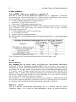
Next, we constructed an EWMA chart of the profit data. We start with plotting the first 25

points to obtain the control limits as shown in Figure 2. One out of limit point was found
and discarded after the derivation of this chart, which was the same project as the outlier on
the normal probability plot (number 5). This was the sole DFSS project (Design for Six
Sigma) in the data base. The others were process improvement projects without design
control. A second graph was developed without the DFSS project point to obtain the chart
shown in Figure 3. These charts were constructed based on Hunter (1989) with λ = 0.40 and
L = 3.054.
Of special interest are the last seven projects. These projects took place after a significant
Six Sigma training program. This provides strong statistical evidence that the training
improved the bottom line of subsequent projects. Such information definitely supports
decisions to invest in training of other divisions. Similar studies with this same technique
could be used to verify whether training contributed to a fundamental change in the
process.

Six Sigma Projects and Personal Experiences

84
Profi t
Percent
40000003000000200000010000000-1000000-2000000
99
95
90
80
70
60
50
40
30
20

10
5
1

Fig. 1. Normal Probability Chart for Six Sigma Projects.

-1500000
-1000000
-500000
0
500000
1000000
1500000
2000000
1 3 5 7 9 1113151719212325
Project
Profit ($)
UCL
zi
LCL
Fig. 2. EWMA Control Chart for first 25 Six Sigma Projects{XE “ system“}.

Analysing Portfolios of Lean Six Sigma Projects

85
-100000
-50000
0
50000
100000

150000
135791113151719212325272931333537
P
r
o
f
i
t

$
Six Sigma Project

Fig. 3. EWMA Control Chart for Six Sigma Projects {XE “ system“}.
3.2 Regression
Many hypotheses can be investigated using regression. Somewhat arbitrarily, we focus on
two types of questions. First, we investigate the appropriateness of applying any type of
method as function of the expected savings. Therefore, regressors include the expected
savings, the total number of formal methods (FM) applied, and whether engineering
analysis (EA) was used. Second, we investigate the effects of training and how projects were
selected. In fitting all models, project 5 caused outliers on the residual plots. Therefore, all
models in this section are based on fits with that (DFSS) project removed.
The following model resulted in an R-squared adjusted equal to 0.88:



Profit $ 22,598.50 1.06´Expected Savin
g
s
2,428.13´FM 5,955.72´EA 0.05´Expected Savin
g

s´FM
0.37´Expected Savings´EA
  


(8)
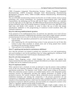
Fig. 4. is based on predictions from equation (8). It provides quantitative evidence for the
common sense realization that applying many methods when engineers do not predict
much savings is a losing proposition.
The model and predictions can be used to set limits on how many methods can be applied
for a project with a certain expected savings. For example, unless the project is expected to
save $50,000, it likely makes little sense to apply multiple formal methods. Also, the model
suggests that relying heavily on engineering analysis for large projects is likely a poor
choice. If the expected saving is higher than $100,000 it is likely not advisable to rely solely
on engineering analysis.

Six Sigma Projects and Personal Experiences

86
$1,600
$490,133
$978,667
$1,467,200
$1,955,733
0
3
6
-$200,000
$0
$200,000

$400,000
$600,000
$800,000
$1,000,000
$1,200,000
$1,400,000
$1,600,000
# Formal
Methods
Used (FM)
Expected Savings
Predicted Profit

Fig. 4. 3D Surface Plot of the Regression Model in Equation (8)

$0
$10,000
$20,000
$30,000
$40,000
$50,000
$60,000
Before
Training
After
Training
Mgt.
Initiated
Individual
Initiated

Predicted Response

Fig. 5. Main Effects Plot of Predictions of the Simple Regression Model{XE “ system“}.
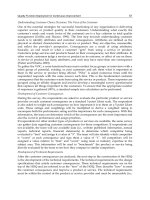
A second regression model was created using the indicator variables:

 if the project was
not influenced by training and

= 1 otherwise and J = 1 if the project was management

Analysing Portfolios of Lean Six Sigma Projects

87
initiate and J = 0 otherwise. This model is represented by equation 9, and shows a positive
correlation between both independent variables non-management initiated and training
with profit:
Profit = 13510 + 38856 I + 19566 J (9)
This model has an adjusted R-squared of only 0.15 presumably because most of the
variation was explained by the variables in equation 8. Note that multicollinearity prevents
fitting a single model accurately with the regressors in both equations. The predictions for
the model in equation (9) are shown in Figure 5.
4. Discussion
The ability to estimate potential effects of changes on the profitability of projects is valuable
information for policymakers in the decision-making process. This study demonstrated that
utilizing existing data analysis tools to this new management data source provides useful
knowledge that could be applied to help guide in project management. Findings included:
 Design for Sigma Projects (DFSS) can be significantly more profitable than process
improvement projects. Therefore, permitting design control can be advisable. In our
study, probability plotting, EWMA charting, and regression all established this result
independently.


Training can significantly improve project performance and its improvement can be
observed using EWMA charts.

Regression can create data-driven standards establishing criteria for how many
methods should be applied as a function of the expected savings.
Also, in our study we compared results of various sized projects and the use of formal tools.
We found that determining the estimate of the economical value to be important to guide
the degree of use of formal tools. Based on the results of this study, when predicted impact
is small, a rapid implementation based on engineering analysis is best. As projects’
predicted impact expands, formal methods can play a larger role.
The simple model also tends to show a strong benefit to training. This model has good
variance inflation factors (VIF) values and supports the findings from the SPC findings. Of
interest is the negative correlation on management initiation of projects. In this regard, there
is still ambiguity in the results. For example, it is not known if people worked harder on
projects they initiated or if they picked more promising projects.
The research also suggests several topics for future research. Replication of the value of the
methods in the context of other companies and industries could be valuable and lead to
different conclusions for different databases. Many other methods could be relevant for
meso-analysis and the effects of sites and the nature of the industry can be investigated.
Many companies have a portfolio of business units and tailoring how six sigma is applied
could be of important interest. In addition, the relationship between meso-analysis and
organizational “resilience” could be studied. These concepts are related in part because
through applying techniques such as control charting, organization might avoid over-
control while reacting promptly and appropriately to large unexpected events, i.e., be more
resilient. Finally, it is hypothetically possible that expert systems could be developed for
data-driven prescription of specific methods for specific types of problems. Such systems
could aid in training and helping organizations develop and maintain a method oriented
competitive advantage.

Six Sigma Projects and Personal Experiences

88
5. Acknowledgment
We thank Clark Mount-Campbell, Joseph Fiksel, Allen Miller, and William Notz for helpful
discussions and encouragement. Also, we thank David Woods for many forms of support.
6. Appendix
This appendix contains the data from the 39 case studies shown in Table 2.

Project Exp. Savings Exp. Time M/I A/P #people EC CH TF PM CE GR
1 $35000 L M A 7 0 1 1 2 1 0
2 $70000 L M A 1 1 1 0 0 0 0
3 $81315 M M A 2 1 1 1 1 0 0
4 $40000 M M A 1 0 0 0 1 0 0
5 $250000 L I P 6 1 1 1 0 2 2
6 $150000 L M P 4 0 1 1 1 0 0
7 $125000 L I P 3 0 1 1 0 0 1
8 $2200000 L M P 9 0 1 0 0 3 0
9 $50000 M M P 5 1 1 1 1 1 1
10 $39195 M M P 1 1 1 0 0 0 0
11 $34500 L M A 1 1 0 0 1 1 1
12 $21000 L M A 1 0 1 0 0 0 0
13 $25000 M M A 1 0 0 0 1 0 0
14 $20000 M M A 1 0 0 0 1 0 0
15 $10000 M M A 1 0 1 0 0 0 0
16 $20000 S M A 1 0 0 0 0 0 0
17 $28000 M I P 1 0 0 0 1 0 0
18 $20000 S M P 5 0 1 1 0 2 0
19 $20000 S M P 1 0 0 0 1 0 0
20 $4350 S M A 1 0 1 0 1 0 0

21 $13750 S M A 1 0 1 0 1 0 0
22 $8500 S M A 1 0 1 0 1 0 0
23 $1600 S M A 1 1 0 0 0 0 0
24 $12500 S M A 1 0 1 0 1 0 0
25 $4000 S M A 1 0 0 0 0 0 0
26 $13000 S M A 1 0 0 0 0 0 0
27 $15000 L I P 1 1 1 0 0 0 0
28 $6000 M I P 1 1 1 0 1 0 0
29 $11500 M I P 2 0 1 1 1 0 0
30 $4500 M I P 1 1 1 0 1 0 0
31 $11000 S M P 5 0 1 1 0 1 0
32 $5400 S M P 5 0 1 1 1 1 0
33 $150000 S I P 4 0 1 0 1 1 1
34 $8600 S I P 2 1 1 0 0 0 0
35 $90000 M M A 5 1 1 1 1 1 1
36 $30000 M M P 7 1 1 1 0 1 0
37 $45000 S M A 3 0 1 0 0 0 1
38 $240000 S I P 3 1 0 0 0 0 0
39 $50000 S I P 4 1 1 0 1 0 0
Table 2. (Continued).

Analysing Portfolios of Lean Six Sigma Projects

89
Project DOE SPC DC FT EA OF Time Cost Act Savings Profit
1 0 0 1 2 0 1 13 $48700 $36000 $-12700
2 1 0 0 1 1 1 18 $7590 $0 $-7590
3 0 0 1 1 1 0 25 $35300 $31500 $-3800
4 0 0 0 0 1 0 20 $2900 $0 $-2900
5 2 0 1 7 0 1 16 $325500 $4E+06 $3874500

6 0 0 1 1 1 0 9 $76000 $170000 $94000
7 1 0 0 2 1 0 7 $17725 $130500 $112775
8 4 0 0 7 4 0 30 $220000 $0 $-220000
9 2 2 1 7 2 1 5.5 $31125 $97800 $66675
10 0 0 1 1 1 1 14 $12350 $19575 $7225
11 0 0 1 3 2 0 18 $22800 $13500 $-9300
12 0 0 0 0 1 0 18 $2600 $0 $-2600
13 0 0 0 0 1 0 18 $2000 $0 $-2000
14 0 0 0 0 1 0 20 $7500 $21740 $14240
15 0 0 1 1 1 1 8 $30800 $17200 $-13600
16 0 0 0 0 1 0 9 $2000 $0 $-2000
17 0 0 2 2 1 0 4 $12000 $7000 $-5000
18 2 1 1 6 0 0 1.5 $5300 $23220 $17920
19 0 0 1 1 1 0 3 $1900 $8050 $6150
20 0 0 1 1 0 0 3 $1000 $4025 $3025
21 0 0 1 1 0 0 3 $1000 $4025 $3025
22 0 0 1 1 0 0 3 $1000 $4025 $3025
23 0 0 1 1 1 1 3 $3525 $3125 $-400
24 0 0 1 1 0 0 3 $3000 $8400 $5400
25 0 0 0 0 1 0 18 $1900 $0 $-1900
26 0 0 0 0 1 0 8 $1900 $0 $-1900
27 1 0 1 2 1 0 19 $12125 $14985 $2860
28 0 0 1 1 1 0 2.5 $1700 $6500 $4800
29 0 1 0 1 1 1 8 $12880 $11700 $-1180
30 0 0 1 1 1 0 4.5 $3060 $6300 $3240
31 1 2 1 5 0 0 3 $4250 $10900 $6650
32 0 1 1 3 0 0 1.5 $2400 $5375 $2975
33 2 0 1 5 1 0 6 $38900 $165440 $126540
34 0 0 1 1 1 0 1 $1500 $10750 $9250
35 1 1 1 5 1 0 3 $12640 $66100 $53460

36 0 0 1 2 1 1 10 $18780 $34056 $15276
37 1 0 1 3 1 1 13 $38584 $46300 $7716
38 0 1 1 2 1 0 12 $15690 $236280 $220590
39 0 0 1 1 0 0 1.5 $1275 $11927 $10652
Table 2. Data From 39 Case Studies with Expected Times Being Short (S), Medium (M), or
Long (L), Management (M) or Individual (I) Initated, Assigned (A) or Participative (P) Team
Selection, and The Numbers of Methods Applied Including Economic Analyses (EC),
Charter (CH) Creations, Total Formal (TF) Design of Experiments or Statistical Process
Control Methods, Process Mapping (PM), Cause & Effect (CE), and Gauge Repeatability and
Reproducibility (GR) Analysis.
7. References
Bisgaard S. and Freiesleben J., Quality Quandaries: Economics of Six Sigma Program,
Quality Engineering, 13 (2), pp. 325-331, 2000.

Six Sigma Projects and Personal Experiences

90
Chan K.K., and Spedding T.A., On-line Optimization of Quality in a Manufacturing System,
International Journal of Production Research, 39 (6): pp. 1127-1145. 2001.
Gautreau N., Yacout S., and Hall R., Simulation of Partially Observed Markov Decision
Process and Dynamic Quality Improvement, Computers & Industrial Engineering,
32 (4): pp. 691-700, 1997.
Harry M.J. A new definition aims to connect quality with financial performance, Quality
Progress, 33 (1) pp. 64-66, 2001.
Harry, M. J., The Vision of Six Sigma: A Roadmap for Breakthrough, 1994 (Sigma Publishing
Company: Phoenix).
Hoerl R. W., Six Sigma Black Belts: What Do They Need to Know? Journal of Quality
Technology, 33 (4): PP. 391-406, 2001a.
Hunter J.S., A one Point Plot Equivalent to the Shewhart Chart with Western Electric Rules,
Quality Engineering, Vol. 2, 1989.

Juran, J. M. and Gryna F., Quality Planning and Analysis, New York: McGraw-Hill, 1980.
Linderman K., Schroeder R.G., Zaheer S. and Choo A.S., Six Sigma: A goal-theoretic
perspective, Journal of Operations Management, 21, (2), pp. 193-203, 2003.
Martin J. A garbage model of the research process, In J. E. McGrath (Ed)., Judgment calls in
research, Beverly Hills, CA: Sage, 1982.
Montgomery D., Editorial, Beyond Six Sigma, Quality and Reliability Engineering
International, 17(4): iii-iv, 2000.
Montgomery D.C., Introduction to Statistical Quality Control, 2004 (John Wiley & Sons, Inc.
New York).
Shewhart W.A. Economic Control of Manufactured Product, New York: D. Van Nostrand,
Inc., 1931.
Yacout S., and Gautreau N., A Partially Observable Simulation Model for Quality
Assurance Policies, International Journal of Production Research, Vol. 38, No. 2,
pp. 253-267, 2000.
Yu B. and Popplewell K., Metamodel in Manufacturing: a Review, International Journal of
Production Research, 32: pp. 787-796, 1994.
5
Successful Projects from the Application
of Six Sigma Methodology
Jaime Sanchez and Adan Valles-Chavez
Instituto Tecnologico de Cd. Juarez
Mexico
1. Introduction
This chapter describes briefly the Six Sigma Methodology (SSM) phases and Key factors for
the effective implementation as well as the important tools. SSM was first introduced by
Motorola in the 1980´s to improve product and service quality through the waste and
variance reduction (Pyzdek, 2003). The SSM is a systematic way to solve problems with
individual projects to attain better profitability. The SSM main objective is to reduce the
number of defective parts to as low as 3.4 parts per million. The objective of this chapter is to
show that taking into account the key factors and applying the right tools profitable results

can be obtained. Three different application cases are used to illustrate the methodology
throughout the chapter and were conducted in twin plants in the Juarez area where the
authors participated.
The SSM is structured in a five steps or phases in order solve successfully quality problems.
These five steps or phases are known as, Define, Measure, Analysis, Improve and Control or
DMAIC procedure. This paper describes these steps and illustrates the Key factors and tools
that are needed for successful applications. The cases are related to applications that have
been published previously (Valles et al., 2009a, 2009b, 2009c) They are design and the
Improvement of Binder manufacturing process, Improvement of automotive speakers
manufacturing process and the implementation of SSM for the manufacturing of a circuit
that is used in inkjet printer cartridges.
The three illustrative applications were successfully implemented by considering the key
factors and important tools used throughout the deployment of the SSM. Also, some
fundamentals were included such as basic definitions and philosophy, efficient
communication, team work, training and management involvement and commitment.
Beside the defective part reductions, some other important results were observed in the
implementation process, such as culture change, trained employees and better human
resources, and better project management skills. In conclusions, there were changes for the
better in all the organizations where the SS implementations were conducted.
2. DMAIC procedure
The DMAIC procedure will be briefly describe in this section (Pande et al., 2002). The SSM
relies on this procedure for the implementation of improvement projects that requires
management commitment and team work. It also involves the use of statistical methods,
quality improvement techniques and the scientific method as well.

Six Sigma Projects and Personal Experiences
92
In the Define step, a team defines the problem objectives and goals, identifies the customers
of the process and customers requirements. The project charter, work plan, measurement of
the customer requirements and process map documentation are needed.

In the Measure step includes the process performance measure selection, measurement
system evaluation and analysis and determination of the process performance level and
capability. In this step what to measure must be decided by the team. Sometimes, it is
difficult to decide, because data collection is even more difficult and time consuming.
The step of Analysis includes the analysis and determination of potential root causes of
variation through the use of statistical tools and the basic quality tools such as Pareto charts,
Ishikawa Diagrams, etc. The phases of the root cause analysis are used in this step. They are
exploring, generating hypotheses about causes and verifying or eliminating causes. The
main input of this step is data generated by the measuring the important variables.
The goal of the Improve step is to find and implement solutions that will eliminate the
causes of problems, reduce variation in a process or prevent a problem from recurring. The
key factor and important tools for the Improve step are identification, evaluation and
verification of potential solutions by the use of basic statistical methods, design of
experiments, response surface, Taguchi methods, etc. The identification of potential
solutions is often generated by brainstorming.
At last, the Control step has the objective to continue measuring the performance of the
process periodically and keeping it under control. The process management control and
action plans are made by implementing control charts, control plans and mistake-proof
devices. It is important to mention that the first three steps are observational studies, that is,
there is not intervention in the process. While in the last two steps are designed
experiments, where the researchers take active action into the process in order to achieve the
established goals.
3. Reduction of the nonconforming fraction in manufacturing of a circuit
The specific objectives of this project were grouped in three categories; measurement
equipment, failure analysis, and process improvement. Regarding the measurement
equipment, the objectives were to evaluate the current measurement system and to assess
the repeatability and reproducibility of the electric tester. In relation to the method of failure
analysis, the objectives were to: evaluate the standardization of criteria for the technical
failures; develop a procedure and sampling plan for defective parts; obtain a reliable
estimate of the distribution for failures in the total population; propose an alternate method

for the analysis of defective parts; and identify and measure the defects, specially the main
electrical defect.
About the analysis of problems and process improvement, the objectives were to; identify
the factors or processes that affect the quality feature in question (electrical function of the
circuit); identify the levels of the parameters in which the effect of the sources of variation
will be minimal; develop proposals for improvement; and to implement and monitor the
proposed improvements.
Definition: During the years 2006 and 2007 the main product had a low level of
performance in electrical test. Historical data shows that on average, 3.12% of the material
was defective. The first step was the selection of the Critical Customer Characteristics and
the response variable. The critical characteristic, in this case, was the internal electrical
defects detected during electrical testing.

Successful Projects from the Application of Six Sigma Methodology
93
Measurement: This phase is to certify the validity of the data through the evaluation of the
measurement system. The first step is a normality test of the data and an analysis of the
process capacity. This began with the measurement of the percentage of electrical failures.
The percentage of electrical failures is obtained after a test is performed to the 100% of
electric circuits.

Repetition Measurement

Moving
Range
Repetition

Measurement

Moving

Range
1 80.1 0 11 80.0 0.2
2 79.9 0.2 12 80.1 0.1
3 80.1 0.2 13 80.1 0
4 79.8 0.3 14 79.9 0.2
5 80.1 0.3 15 79.9 0
6 80.1 0 16 80.0 0.1
7 79.9 0.2 17 79.8 0.2
8 80.2 0.3 18 79.8 0
9 80.1 0.1 19 80.1 0.3
10 79.8 0.3 20 80.0 0.1
Table 1. Measured by Operator (Reference Value of 73.5 Ohms)
In order to evaluate the accuracy of the equipment, a standard piece was used with a
reference value of 75.3 Ω, which was measured 20 times by the same operator. According to
the results of the data shown in Table 1, it is concluded that a 0.05% accuracy of the
calibration of the instrument is acceptable.
The evaluation of the capability of the measurement process in terms of precision was
conducted through a study of repeatability and reproducibility (R&R). The evaluation was
conducted with 10 pieces of production taken at different hours, with 3 operators and 3
repetitions. The results of the R&R study was performed with Minitab© shown in Table 2.
The total variability introduced by the electrical tester is 3.32%, which is considered
excellent.

Source StdDev Study Var
(6 * SD)
%Study Var
(%SV)
%Tolerance
(SV/Toler)
%Process

(SV/Proc)
Total Gauge
R&R
4.43E-02 0.265832 48.59 3.32 28.90
Repeatability 3.78E-02 0.232379 42.47 2.90 25.26
Reproducibility 2.15E+00

0.129099 23.60 1.61 14.04
Operator 0.00E+00

0.000000 0.00 0.00 0.00
Operator*Part 2.15E-02 0.129099 23.60 1.61 14.04
Part-To-Part 7.97E-02 0.478191 87.40 5.98 51.99
Total Variation 9.12E-02 0.547114 100.00 6.84 59.48
Table 2. Results of the Repeatability and Reproducibility Study
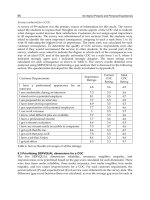
A study of repeatability and reproducibility for attributes was done with purpose of
ensuring the consistency of the criteria used by four different inspection areas. Table 3
shows the result.

Six Sigma Projects and Personal Experiences
94
Evaluatio
n

Shift A
Ins
p
ector

Shift B

Ins
p
ector

Shift C
Ins
p
ector

Shift D
Ins
p
ector
% Matched

96.67%

96.67%

93.33%

90.00%
%Appraised Vs. known
standard

93.33%

93.33%

86.66%

76.67%
Table 3. Study of Repeatability and Reproducibility for Attributes
Analysis: This phase consisted of searching through brainstorming rounds the possible
factors that may be affecting the electrical performance of the product. The factors that were
considered most important were raised as hypotheses and verified by different statistical
tests. The objective was to identify key factors of variation in the process. For the
identification of potential causes were prepared Pareto Charts of Defects, in one of them,
about 33% of the electrical faults analyzed cannot be identified with the test equipment and
21.58% are attributed to the defect called "Waste of Aluminum Oxide”, given that the
current equipment does not detect 33% of nonconformities. Samples were sent to an external
laboratory, observing that more than 50% of the parts had traces of aluminum oxide so
small that they could not be detected with the microscope used in the laboratory of failure
analysis. Because this waste may cause several problems, a cause and effect matrix shown in
Table 4 was prepared to prioritize areas of focus.
The causes considered important were; the quantity of wash cycles, the thickness of the
Procoat layer, Lots circuit, the parameters of grit blast equipment and the operational
differences among shifts. With respect to the quantity of wash cycles, to determine if they
affect the fraction of electrical defects, an experiment with, one, two and three wash cycles as
factor levels with sample sizes of 30 wafers each. Data was tested for normality. The
statistical differences among wash cycles are not significant, concluding that Wash Cycle is
not an important factor. The results of these tests are not shown. In relation to the thickness
of the Procoat finish, it was suspected that the increase of the thickness reduces the
percentage of electrical failures. This is to reduce the impact that grains of aluminum oxide
has on the semiconductor. An experiment with a single factor was carried out. The factor
assessed was the thickness of the layer of Procoat under 4 levels and 30 replications. The 120
runs were conducted completely random. The different thicknesses of Procoat tested were 0,
14, 30, 42 microns. The results of the Anova for this experiment are shown in Figure 1.
The data indicate that there is a difference between the levels, as the p-value is less or equal
to 0.0001. Only the level of 0 micron is different from the others and the confidence intervals

of the other three levels overlap, then they have the same mean. Figure 2 shows the
comparisons of the four levels of procoat in relation to the percentage of electrical failures.
The layer of procoat improves electrical performance up to 14 microns (a condition of the
current process); however it is not justifiable to increase the thickness of the layer, as it did
not represent improvement in the average electric performance or to reduce the variation.
Concerning the Lots of raw material for the Circuit, in order to prove that the condition of
the raw material is not a factor that is influencing the electrical performance, it was
necessary to verify the following hypotheses: H
0
: There is no difference in the fraction of
defective units between different batches vs. H
1
: There is a difference in the fraction of
defective units between different batches. Because the four lots of raw material that were
selected randomly contain different amounts of wafers, the experiment was an unbalanced
completely random design. Each batch contains between 20 and 24 wafers. In a shift 200

Successful Projects from the Application of Six Sigma Methodology
95
circuits can be assembled. Each circuit is mounted in a cartridge for inkjet printers that are
electrically tested on an individual basis. The ANOVA results are summarized in Figure 2,
indicating that there is no difference in the percentage of electrical failures of wafers per
batch. The P-Value of 0. 864 is a high probability that the lots have equal means. Therefore,
the null hypothesis is not rejected. Then it is concluded that the lots of wafers show no
difference in electric behavior and the assumption that some batches posses a lower
electrical performance is discarded.

Cause and Effect Matrix
Rating of Importance to
Costumers

5.91 2.3 1 0.78

Y´s 1 2 3 4 5


Residual
AIO
Scratch

Tester
Error
Pad
Contamination

Requirement

Total

X´s
Process
Step
Process Input


1 Grit Blast 9 9 0 3

75.96

2
Nozzle

Attached
6 6 0 6

53.76

3 Lexfilm 0 9 0 9

27.45

4 Electrical Test

0 0 9 0

9.36
5 Dicing 0 3 0 0

6.81
6 Tab Bond 0 0 0 0

0

Total 89 61 9 14

Table 4. Cause-Effect Matrix


Fig. 1. Results of the ANOVA for the Procoat Layer Thickness
Additionally, the test of equal variances (for the four lots) concluded that there is no hard
evidence to suggest that the variability in the percentage of electrical failures depends on the
lot or semiconductor wafers. Figure 3 shows the results of Bartlett test, where the p-value of

0.926 (P> 0.05). Data was tested for normality before the test the hypothesis of equality of
the averages of the batches with an ANOVA. There was no evidence to say that the data was
not normally distributed.