Superconductivity Theory and Applications Part 4 potx

Superconductivity – Theory and Applications
64

Fig. 6. The panels on the left (a)-(c) show the ’’(T) response for different H. The right hand
panels (d)-(f), show the derivative d’’/dT determined from the corresponding ’’(T) curves
on the left panel. (see discussion in the text) [Mohan et al. 2007; Mohan 2009b]
In Fig.5(c), for H= 12500 Oe, three distinct regimes of behaviour in the ’’(T) response have
been identified as the regions 1, 2 and 3. Region 1 is characterized by a high dissipation
response. As noted earlier, this high dissipation results from full penetration of h
ac
to the
center of the sample, similar to the dissipation peak marked at A in Fig.3(b). As noted earlier
in Fig.5(a), at these high fields beyond 1000 G, at T > T
cr
, ’(T) response possesses no distinct
signature of the PE phenomenon. The absence of any distinct PE feature in ’(T) should have
caused no modulations in the behavior of ’’(T) response, except for a peak in dissipation
close to T
c
(H). Instead, in the region 2 (cross shaded and located between the T
cr
and T
fl

arrows in Fig.5(c)) a new behaviour in the dissipation response is observed, viz., in this
region there is a substantial decrease in dissipation.
As seen earlier in the context of PE in Fig.3(b), that any anomalous increase in pinning
corresponds to a decrease in the dissipation. The observation of a large drop in dissipation
across T
cr

(Fig.5(c)) indicates there is a transformation from low J
c
state to a high J
c
state, i.e.,
a transformation from weak pinning to strong pinning. Subsequent to the drop in ’’(T) in

Nonlinear Response of the Static and Dynamic Phases of the Vortex Matter
65
region 2, the dissipation response attempts to show an abrupt increase (see change in slope
in d’’/dT in Fig.6(d) to (f)) at the onset of region 3 (marked as T
fl
in Fig.5 and Fig.6). The
abrupt increase in dissipation beyond T
fl
is more pronounced at low H and high T (see
behavior in Fig.5(b)). The significance of T
fl
will be revealed in subsequent sections. In brief,
the T
fl
will be considered to identify the onset of a regime dominated by thermal
fluctuations, where pinning effects become negligible and dissipation response goes through
a peak. It is interesting to note that the T
fl
locations are identical to the location of T
p
(viz.,
the peak of PE) in Figs.5(a) and 5(c). For H < 750 Oe, the T
fl

location can be identified with
the appearance of a distinct PE peak at T
p
(see Fig.4, where dissipation enhances at T
p
= T
fl
).
It is important to reiterate that the anomalous drop in dissipation in region 2 near T
cr
is not
associated with the PE phenomenon.


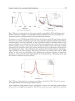
Fig. 7. The real (a) and imaginary (b) parts of the ac susceptibility measured in the ZFC and
FC modes, for H = 1000 Oe. Also marked for are the locations of the T
cr
and T
fl
. [Mohan et
al. 2007; Mohan 2009b]
All the above discussions pertain to susceptibility measurements performed in the zero field
cooled (ZFC) mode. Detailed studies of the dependence of the thermomagnetic history
dependent magnetization response on the pinning (Banerjee et al. 1999b, Thakur et al.,
2006), had shown an enhancement in the history dependent magnetization response and
enhanced metastablility developing in the vortex state as the pinning increases across the
PE. While the ZFC and field cooling (FC), ’(T) response can be identical in samples with
weak pinning, the will show that ’’(T) is a more sensitive measure of small difference in the
thermomagnetic history dependent response. Figures 7(a) and 7(b) display ’(T) and ’’(T)
measured for a vortex state prepared either in ZFC or FC state in 1000 Oe. Figure 7(a) shows

the absence of PE at T
cr
in the ’(T) response at 1000 Oe for vortex state prepared in both FC
and ZFC modes. Furthermore, there is no difference between the ZFC and FC ’(T)

Superconductivity – Theory and Applications
66
responses (cf.Fig.7(a)). However, the dissipation (’’(T)) behaviour in the two states
(Fig.7(b)) are slightly different. While there are no clear signatures of T
cr
in the ’(T)
response, in ’’(T) response (Fig.7(b)) below T
cr
one observes that the FC response
significantly differs from that of the ZFC state, with the dissipation in the FC state below T
cr

being lower as compared to that in the ZFC state. The presence of a strong pinning vortex
state above T
cr
, causes the freezing in of a metastable stronger pinned vortex state present
above T
cr
,

when the sample is field cooled to T < T
cr
. As the FC state has higher pinning than
the ZFC state (which is in a weak pinning state) at the same T below T
cr

, therefore, the ’’(T)
response is lower for the FC state. Above T
cr
the behavior of ZFC and FC curves are
identical, as both transform into a maximally pinned vortex state above T
cr
. The behavior of
’’(T) in the FC state indicates that the pinning enhances across T
cr
. Beyond T
cr
, the ZFC and
FC curves match and the high pinning regime exists till T
fl
. This observation holds true for
all H
dc
above 1000 Oe as well.
3.2.1 Transformation in pinning: evidence from DC magnetization measurements
Figure 8 displays measured forward (M
fwd
) and (M
rev
) reverse magnetization responses of
2H-NbSe
2
at temperatures of 4.4 K, 5.4 K and 6.3 K for H  c.


Fig. 8. The M-H hysteresis loops at different T. (a) The forward and reverse legs of the M-H

loops are indicated as M
fwd
and M
rev
. (b) in M
rev
(H) array at different T. The locations of the
observed humps in the M
rev
(H) curves are marked with arrows. Also indicated, in the 6.3 K
curve, is the location of the field that corresponds to the temperature, T
fl
= T
irr
. [Mohan et al.
2007; Mohan 2009b]
A striking feature of the M-H loops in Fig. 8 is the asymmetry in the forward (M
fwd
) and
reverse (M
rev
) legs. The M
rev
leg of the hysteresis curve exhibits a change in curvature at low
fields. In Fig.8(b) we plot only the M
rev
from the M-H recorded at 4.4 K, 5.4 K and 6.3 K. At
low fields, the M
rev
leg exhibits a hump; the location of the humps are denoted by arrows in

Fig.8(b). The characteristic hump-like feature (marked with arrows in Fig.8(b)) can be
identified closely with T
cr
locations identified in Figs.4, 5 and 6. The tendency of the
dissipation ’’ to rapidly rise close to T
fl
(H) (cf. Figs.4, 5 and 6) is a behaviour which is
expected across the irreversibility line (T
irr
(H)) in the H-T phase diagram, where the bulk
pinning and, hence, the hysteresis in the M(H) loop becomes undetectably small. The
decrease in pinning at T
irr
(H), results in a state with mobile vortices which are free to

Nonlinear Response of the Static and Dynamic Phases of the Vortex Matter
67
dissipate. We have confirmed that T
fl
(H) coincides with T
irr
(H), by comparing dc
magnetization with ’’ response measurements (cf. arrow marked as T
fl
= T
irr
in Fig.8 for the
6.3 K curve). Thus T
fl
(H) coincides with T

irr
(H), which is also where the peak of the PE
occurs, viz., the peak of PE at T
p
occurs at the edge of irreversibility (cf. H-T phase diagram
in Fig.9).
3.3 The H-T vortex phase diagram and pinning crossover region
Figure 9(a) shows the H

- T, vortex matter phase diagram wherein we show the location of
the T
c
(H) line which is determined by the onset of diamagnetism in (T), the T
p
(B) line
which denotes the location of the PE phenomenon, the T
cr
(H) line across which the (T)
response (shaded region 2 in Fig.5(c)) shows a substantial decrease in the dissipation and
the T
fl
line beyond which dissipation attempts to increase. The PE ceases to be a distinct
noticeable feature beyond 750 G and the T
p
(H) line (identified with arrows in Fig. 5(a))
continues as the T
fl
(H) line. Note the T
fl
(H) line also coincides with T

irr
(H). For clarity we
have indicated only the T
fl
(H) line in the phase diagram with open triangles in Fig.9(a).


(a) (b)
Fig. 9. (a) The phase diagram showing the different regimes of the vortex matter. The inset is
a log-log plot of the width of the hysteresis loop versus field at 6K. (b) An estimate of
variation in J
c
with f
p
/f
Lab
in different pinning regimes. [Mohan et al. 2007; Mohan 2009b].
We consider the T
cr
(H) line as a crossover in the pinning strength experienced by vortices,
which occurs well prior to the PE. A criterion for weak to strong pinning crossover is when
the pinning force far exceeds the change in the elastic energy of the vortex lattice, due to
pinning induced distortions of the vortex line. This can be expressed as (Blatter et al, 2004),
the pinning force (f
p
) ~ Labusch force (f
Lab
) = (
0
/a

0
), where 
0
= (
0
/4)
2
is the energy
scale for the vortex line tension,  is the coherence length, 
0
flux quantum associated with a
vortex,  is the penetration depth and a
0
is the inter vortex spacing (a
0
 H
-0.5
). A softening of
the vortex lattice satisfies the criterion for the crossover in pinning. At the crossover in
pinning, we have a relationship, a
0
 
0
 f
p
-1
. At H
cr
(T)

and far away from T
c
, if we use a
monotonically decreasing temperature dependent function for f
p
~ f
p0
(1-t)

, where t=T/T
c
(0)
and  > 0, then we obtain the relation H
cr
(T)  (1-t)
2

. We have used the form derived for
H
cr
(T) to obtain a good fit (solid line through the data Fig.9(a)) for T
cr
(B) data, giving 2~
1.66  0.03. Inset of Fig. 9(a) is a log-log plot of the width of the magnetization loop (M)

Superconductivity – Theory and Applications
68
versus H. The weak collective pinning regime is characterized by the region shown in the
inset, where the measured M(H) (red curve) values coincide with the black dashed line,
viz.,

1
c
p
MJ
H
 , with p as a positive integer (discussed earlier). Using expressions for
J
c
(f
p
/f
Lab
) (Blatter, 2004), a
0
~  and = 2300 A, = 23 A for 2H-NbSe
2
(Higgins and
Bhattacharya, 1996) and parameters like density of pins suitably chosen to reproduce J
c

values comparable to those experimentally measured for 2H-NbSe
2
, Fig.9(b) shows the
enhancement in J
c
expected at the weak to strong pinning regime, viz., around the shaded
region in Fig.9(b) marked J
c
, in the vicinity of f
p

/f
Lab
~ 1. In Fig.9(a), the shaded region in
the M(H) ( J
c
(H), Bean, 1962; 1967) plot shows the excess pinning that develops due to the
pinning crossover across H
cr
(T) ( T
cr
(H)). Comparing Figs.9(b) and 9(a) we find Jc/J
c,weak

~ 1 compares closely with the (change in M in shaded region ~ 0.6 T in Fig.9(a) inset)/ M
(along extrapolated black line ~ 0.6 T) ~ 0.5. In the PE regime, usually Jc/J
c,weak
 10 (see
for example in Fig.2). Note from the above analysis and the distinctness of the T
cr
and T
p

lines in Fig.9(a), shows that the excess pinning associated with the pinning crossover does
not occur in the vicinity of the PE, rather it is a line which divides the elastically pinned
regime prior to PE. Based on the above discussion we surmise that the T
cr
(H) line marks the
onset of an instability in the static elastic vortex lattice due to which there is a crossover
from weak (region 1 in Fig.5(c)) to a strong pinning regime (region 2 in Fig.5(c)). The
crossover in pinning produces interesting history dependent response in the

superconductor, as seen in the M
rev
measurements of Fig. 8 and in the (T) response for the
ZFC and FC vortex states, in the main panel of Fig.7. In the inset (b) of Fig.8 we have
schematically identified the pinning crossover (by the sketched dark curved arrows in
Fig.8(b)) by distinguishing two different branches in the M
rev
(H) curve, which correspond to
magnetization response of vortex states with high and low J
c
. We reiterate that the onset of
instability of the elastic vortex lattice sets in well prior to PE phenomenon without
producing the anomalous PE.
As the strong pinning regime commences upon crossing H
cr
, how then does pinning
dramatically enhance across PE? The T
fl
(H) line in Fig.9 marks the end of the strong pinning
regime of the vortex state. Above the T
fl
(H) line and close to T
c
(H), the tendency of the
dissipation response to increase rapidly (Figs.1 and 2) especially at low H and high T,
implies that thermal fluctuation effects dominate over pinning. We find that our values (H
fl
,
T
fl

) in Fig.9(a), satisfies the equation governing the melting of the vortex state, viz.,
2
2
4
2
2
(0) 1
(0)
fl fl
c
L
fl m c
iflcc
TB
T
c
BH
GTTH

















, where,

m
= 5.6 (Blatter et al, 1994),
Lindemann no. c
L
~ 0.25 (Troyanovski et al. 1999, 2002),
2
(0)
c
c
H

= 14.5 T, if a parameter, G
i
is
in the range of 1.5 x 10
-3
to 10
-4
. The Ginzburg number, G
i
, in the above equation controls the
size of the H - T region in which thermal fluctuations dominate. A value of O(10
-4
) is

expected for 2H-NbSe
2
(Higgins & Bhattacharya, 1996). The above discussion implies that
thermal fluctuations dominate beyond T
fl
(H). By noting that T
p
(H) appears very close to
T
fl
(H), it seems that PE appears on the boundary separating strong pinning and thermal
fluctuation dominated regimes.
The above observations (Mohan et al, 2007) imply that instabilities developing within the
vortex lattice lead to the crossover in pinning which occurs well before the PE. Infact, PE

Nonlinear Response of the Static and Dynamic Phases of the Vortex Matter
69
seems to sit on a boundary which separates a strong pinning dominated regime from a
thermal fluctuation dominated regime. These assertions could have significant ramifications
pertaining to the origin of PE which was originally attributed to a softening of the elastic
modulii of the vortex lattice. Even though thermal fluctuations try to reduce pinning, we
believe newer results show that at PE, the pinning and thermal fluctuations effects combine
in a non trivial way to dramatically enhance pinning, much beyond what is expected from
pinning crossovers. The change in the pinning response deep in the elastic vortex state is
expected to lead to nonlinear response under the influence of a drive. It is interesting to ask
if these crossovers and transformation in the static vortex state evolve and leave their
imprint in the driven vortex state.
4 Nonlinear response of the moving vortex state
4.1 I-V characteristics and the various phases of the driven vortex matter
In the presence of an external transport current (I) the vortex lattice gets set into motion. A

Lorentz force,
f
L
=J x 
0
/c, acting on each vortex due to a net current density J (due to current
(I) sent through the superconductor and the currents from neighbouring vortices) sets the
vortices in motion. As the Lorentz force exceeds the pinning force, i.e f
L
>f
p
, the vortices begin
to move with a force-dependent velocity, v. The motion of the flux lines induces an electric
field
E = B x v, in the direction of the applied current causing the appearance of a longitudinal
voltage (V) across the voltage contacts (Blatter et al, 1994). Hence, the measured voltage, V in a
transport experiment can be related to the velocity (v) of the moving vortices via V=Bvd,
where d is the distance between the voltage contacts. Measurements of the V (equivalent to
vortex velocity v) as a function of I, H, T or time (t) are expected to reveal various phases and
their associated characteristics an nonlinear behavior of the driven vortex state.
When vortices are driven over random pinning centers, broadly, four different flow regimes
have been established theoretically and through significantly large number of experiments
(Shi & Berlinski 1991; Giammarchi & Le Doussal, 1996; Le Doussal & Giammarchi, 1998;
Giammarchi & Bhattacharya, 2002). These are: (a) depinning, (b) elastic flow, (c) plastic
flow, and (e) the free-flow regime. At low drives, the depinning regime is first encountered,
when the driving force just exceeds the pinning force and the vortices begin moving. As the
vortex state is set in motion near the depinning regime, the moving vortex state is
proliferated with topological defects, like, dislocations (Falesky et al, 1996). As the drive is
increased by increasing the current through the sample, the dislocations are found to heal
out from the moving system and the moving vortex state enters an ordered flow regime

(Giammarchi & Le Doussal, 1996; Yaron et al., 1994; Duarte, 1996). The depinning regime is
thus followed by an elastically flowing phase at moderately higher drives, when all the
vortices are moving almost uniformly and maintain their spatial correlations. The nature
and characteristics of this phase was theoretically described as the moving Bragg glass
phase (Giammarchi & Le Doussal, 1996; Le Doussal & Giammarchi, 1998). In the PE regime
of the H- T phase diagram, it is found that as the vortices are driven, the moving vortex state
is proliferated with topological defects and dislocations, thereby leading to loss of
correlation amongst the moving vortices (Falesky et al, 1996; Giammarchi & Le Doussal,
1996; Le Doussal & Giammarchi, 1998; Giammarchi & Bhattacharya 2002). This is the regime
of plastic flow. In the plastic flow regime, chunks of vortices remain pinned forming islands
of localized vortices, while there are channels of moving vortices flowing around these
pinned islands, viz., different parts of the system flow with different velocities

Superconductivity – Theory and Applications
70
(Bhattacharya & Higgins, 1993, Higgins & Bhattacharya 1996; Nori, 1996; Tryoanovski et al,
1999). The effect of the pins on the moving vortex phase driven over random pinning
centers is considered to be equivalent to the effect of an effective temperature acting on the
driven vortex state. This effective temperature has been theoretically considered to lead to a
driven vortex liquid regime at large drives (Koshelev & Vinokur, 1994). At larger drives, the
vortex matter is driven into a freely flowing regime. Thus, with increasing drive, interplay
between interaction and disordering effects, causes the flowing vortex matter to evolve
between the various regimes.
The plastic flow regime has been an area of intense study. The current (I) - voltage (V)
characteristics in the plastic flow regime across the PE regime are highly nonlinear (Higgins
& Bhattacharya, 1996), where a small change in I is found to produce large changes in V.
Investigations into the power spectrum of V fluctuations revealed significant increase in the
noise power on entering the plastic flow regime (Marley, 1995; Paltiel et al., 2000, 2002). The
peak in the noise power spectrum in the plastic flow regime was reported to be of few Hertz
(Paltiel et al., 2002). The glassy dynamics of the vortex state in the plastic flow regime is

characterized by metastability and memory effects (Li et al, 2005, 2006; Xiao et al, 1999). An
edge contamination model pertaining to injection of defects from the nonuniform sample
edges into the moving vortex state can rationalise variety of observations associated with
the plastic flow regime (Paltiel et al., 2000; 2002). In recent times experiments (Li et al, 2006)
have established a connection between the time required for a static vortex state to reach
steady state flow with the amount of topological disorder present in the static vortex state.
By choosing the H-T regime carefully, one finds that while the discussed times scales are
relatively short for a well ordered static vortex state, the times scales become significantly
large for a disordered vortex state set into flow, especially in the PE regime. The discovery
of pinning transformations deep in the elastic vortex state (Mohan et al, 2007), motivated a
search for nonlinear response deep in the elastic regime as well as to investigate the time
series response in the different regimes of vortex flow (Mohan et al, 2009).
4.2 Identification of driven states of vortex matter in transport measurements
The single crystal of 2H-NbSe
2
used in our transport measurements (Mohan et al, 2009) had
pinning strength in between samples of A and B variety (see section 2.1.1). The dc magnetic
field (H) applied parallel to the c-axis of the single crystal and the dc current (I
dc
) applied
along its ‘ab’ plane (Mohan et al, 2009). The voltage contacts had spacing of d ~ 1 mm apart.
Figure 10(a) shows the plots of resistance (R=V/I
dc
) versus H at 2.5 K, 4 K, 4.5 K, 5 K, 5.8 K
and 6 K measured with I
dc
=30 mA. With increasing H, all the R-H curves exhibit common
features viz., nearly zero R values at lowest H, increasing R after depinning at larger H, an
anomalous drop in R associated with onset of plastic flow regime and finally, a transition to
the normal state at high values of H. To illustrate in detail these main features, and to

identify different regime of driven vortex state, we draw attention only to the 5 K data in
Figure 10(b).
At 5 K, for H < 1.2 kOe, R < 0.1 m
, which implies an immobile, pinned vortex state.
Beyond 1.2 kOe (position marked as H
dp
in Fig.10(b)), the FLL gets depinned and R
increases to m
 range. From this we estimate the critical current I
c
to be 30 mA (at 5 K, 1.2
kOe). The enhanced pinning associated with the anomalous PE phenomenon leads to a drop
in R starting at around 6 kOe (onset location marked as H
pl
) and continuing up to around 8
kOe (location marked as H
p
). The PE ( plastic flow) region is shaded in Fig.10(b). As


Nonlinear Response of the Static and Dynamic Phases of the Vortex Matter
71

Fig. 10. (a) R versus H (H \\ c) of the vortex state, measured at different T with I
dc
=30 mA.
(b) R-H at 5 K only, with the different driven vortex state regimes marked with arrows. The
arrows marks the locations of, depinning (H
dp
), onset of plastic deformations (H

p
), peak
location of PE (H
p
) and upper critical field (H
c2
) at 5 K, respectively. The inset location of
above fields (Fig.10(b)) on the H-T diagram. [Mohan et al. 2009a; Mohan 2009b].

Fig. 11. (a) The V-I
dc
characteristics and dV/dI
dc
vs I
dc
in the elastic phase at 4 K and 7.6 kOe.
The solid line is a fit to the V-I
dc
data, (cf. text for details). (b) R-H curve at 4.5 K and I
dc
= 30
mA. [Mohan et al. 2009a; Mohan 2009b]
discussed earlier (Fig.9), beyond H
p
, thermal fluctuations dominate causing large increase in
R associated with pinning free mobile vortices until the upper critical field H
c2
is reached.
We determine H
c2

(T) as the intersection point of the extrapolated behaviour of the R-H
curve in the normal and superconducting states, as shown in Fig.10(b). By identifying these
features from the other R-H curves (Fig.10(a)), an inset in Fig.10(b) shows the H-T vortex
phase diagram for the vortex matter driven with I
dc
= 30 mA.
Figure 11 shows the V-I
dc
characteristics at 4 K and 7.6 kOe; this field value lies between
H
dp
(T) and H
pl
(T) (see inset, Fig.10(b)), i.e. in the elastic flow regime. It is seen that the data
fits (see solid line in Fig.11(a)) to V~(I
dc
- I
c
)

, where  ~ 2 and I
c
= 18 mA (I = I
c
, when V ≥ 5
V, as V develops only after the vortex state is depinned), which inturn indicates the onset
of an elastically flow. Experiments indicate the concave curvature in I-V coincides with
ordered elastic vortex flow (Duarte et al, 1996; Yaron et al.,1994; Higgins and Bhattacharya
1996). Unlike the elastic flow regime, the plastic flow regime is characterized by a convex

Superconductivity – Theory and Applications
72
curvature in the V-I
dc
curve alongwith a conspicuous peak in the differential resistance
(Higgins and Bhattacharya, 1996), which is absent in Fig.11 (see dV/dI
dc
vs I
dc
in Fig.11(a)).
All the above indicate ordered elastic vortex flow regime at 4 K, 7.6 kOe and I = 30 mA. The
dV/dI
dc
curve also indicates a nonlinear V-I
dc
response deep in the elastic flow regime.
4.3 Time series measurements of voltage fluctuations and its evolution across
different driven phases of the vortex matter
Figure 11(b), shows the R-H curve for 4.5 K. Like Fig.10(b), in Fig. 11 (b), the H
dp
, H
pl
, H
p

and H
c2
locations are identified by arrows, which also identify the field values, at which
time series measurements were performed. The protocol for the time series measurements
was as follows: At a fixed T, H and I

dc
, the dc voltage V
0
across the electrical contacts of the
sample was measured by averaging over a large number of measurements ~ 100. The V
0

measurement prior to every time series measurement run, ensures that we are in the desired
location on R-H curve, viz., the V
0
/I value measured before each time series run should be
almost identical to the value on the R(H) curve at the given H,T, like the one shown in
Figs.10(b) or 11(b). After ensuring the vortex state has acquired a steady flowing state, viz.,
by ensuring the mean V,i.e., <V> ~ V
0
, the time series of the voltage response (V(t)) is
measured in bins of 35 ms for a net time period of a minute, at different H, T.


Fig. 12. (a) The left most vertical column of panels represent the fluctuations in voltage
V(t)/V
0
measured at different fields at 4.5 K with I
dc
of 30 mA. Note: V
0
(2.6 kOe) = 1.4 V,
V
0
(3 kOe) = 3.7 V, V

0
(3.6 kOe) = 9.5 V, V
0
(5 kOe) = 21.1 V, V
0
(7.6 kOe) = 50.7 V. The
middle set of panels are the C(t) calculated from the corresponding V(t)/V
0
panels on the
left. The right hand set of panels show the amplitude of the FFT spectrum calculated from
the corresponding C(t) panels. In Fig.12 (b), the organization of panels is identical to that in
Fig.12 (a) with, V
0
(8 kOe) = 54.5 V, V
0
(9.6 kOe) = 9.8 V, V
0
(10 kOe) = 1.0 V, V
0
(10.8 kOe)
= 0.2
V, V
0
(12 kOe) = 3.2 V. [Mohan et al. 2009a; Mohan 2009b]
The time series V(t) measurements at T=4.5 K are summarised in Figs.12 (a), Fig.12 (b), Fig.
13 (a) and Fig.13 (b). The stack of left hand panels in Figs. 12(a), 12(b), 13(a) and 13(b) show
the normalized V(t)/V
0
versus time (t) for different driven regimes, viz., the just depinned
state (H ~ H

dp
), the freely flowing elastic regime (H
dp
<H < H
pl
), above the onset of the

Nonlinear Response of the Static and Dynamic Phases of the Vortex Matter
73
plastic regime (H > H
pl
), deep inside the plastic regime (H ~ H
p
) and above PE regime (H >
H
p
) (cf. Fig.11(b)). A striking feature in these panels is the amplitude of fluctuations in V(t)
about the V
0
value are significantly large, varying between 10-50% of V
0
, depending on the
vortex flow regime. As one approaches very near to the normal regime, the fluctuations in
V(t) are about 1% of V
0
(see bottom most plot at 16 kOe the left stack of panels in Fig.13(a))
and is about 0.02% deep inside the normal state (see Fig. 13(b), left panel). Near H
dp
(2.6 kOe
and 3 kOe, Fig.12(a)) the fluctuations are not smooth, but on entering the elastic flow

regime, one can observe spectacular nearly-periodic oscillations of V(t) (see at 3.6 kOe, 5 kOe
and 7.6 kOe in panels of Fig.12(a)). Such conspicuously large amplitude, slow time period
fluctuations of the voltage V(t), which are sustained within the elastically driven state of the
vortex matter (up to 7.6 kOe), begin to degrade on entering the plastic regime (above 8 kOe,
see Fig.12(b)).


Fig. 13. (a) consists of three columns representing V(t)/V
0
, C(t) and power spectrum of
fluctuations (see text for details) measured with I
dc
of 30 mA. Note: V
0
(12.4 kOe) = 13.6 V,
V
0
(12.8 kOe) = 49.6 V, V
0
(13.6 kOe) = 284.9 V, V
0
(14 kOe) = 404.5 V, V
0
(16 kOe) = 513.7
V. (b)Panels show similar set of panels as (a) in the normal state at T = 10 K and H = 10 kOe
with I
dc
of 30 mA (V
0
= 539. 6 V). [Mohan et al. 2009a; Mohan 2009b]

Considering that the voltage (V) developed between the contacts on the sample is
proportional to the velocity (v) of the vortices (see section 4.1, V=Bvd), therefore to
investigate the velocity – velocity correlations in the moving vortex state, the voltage-
voltage (
 velocity – velocity) correlation function:
)()(
1
)(
2
0
tVttV
V
tC 


, was determined
from the V(t)/V
0
signals (see the middle sets of panels in Figs.12 (a) and 12 (b) and Fig. 13
for the C(t) plots). In the steady flowing state, if all the vortices were to be moving
uniformly, then the velocity – velocity correlation (C(t)) will be featureless and flat. While if
the vortex motion was uncorrelated then they would lose velocity correlation within a short
interval of time after onset of motion, then the C(t) would be found to quickly decay. Note
an interesting evolution in C(t) with the underlying different phases of the vortex matter.
While there are almost periodic fluctuations in C(t) at 3.6 kOe, 5 kOe and 7.6 kOe (at H <
H
pl
) sustained over long time intervals, there are also intermittent quasi-periodic

Superconductivity – Theory and Applications

74
fluctuations sustained for a relatively short intervals even at H > H
pl
, viz., at 10.8 kOe and
13.6 kOe (see Fig.12 and Fig.13). The periodic nature of C(t) indicates that in certain regimes
of vortex flow, viz., even deep in the driven elastic regime (viz., 3.6 kOe, 5 kOe and 7.6 kOe
in Fig.12(a) panels) the moving steady state of the vortex flow, the vortices are not always
perfectly correlated. Instead their velocity appears to get periodically correlated and then
again drops out of correlation.
Once can deduce the power spectrum of the fluctuations by numerically determining the
fast Fourier transform (FFT) of C(t). The FFT results are presented in the right hand set of
panels in Figures 12(a), 12(b), 13(a) and 13(b). A summary of the essential features of the
power spectrum are as follows. At 2.6 kOe where the vortex array is just above the
depinning limit for I
dc
= 30 mA, one finds two peak-like features in the power spectrum
centered around 0.25 Hz and 2 Hz (Fig.12(a)). With increasing field, the peak feature at 2 Hz
vanishes, and with the onset of freely flowing elastic regime (>3 kOe), a distinct sharp peak
located close to 0.25 Hz survives. This low-frequency peak, which exists up to H = 7.6 kOe,
has an amplitude nearly five times that at 0.25 Hz for 2.6 kOe. In the plastic flow regime,
viz., H > H
pl
~ 8 kOe, the amplitude of the 0.25 Hz frequency starts diminishing (Figs.12(b),
the right most panel). At the peak location of the PE (H
p
=10.8 kOe), the 0.25 Hz frequency is
absent but there is now a well defined peak in the power spectrum close to 2 Hz (see
Fig.12(b)). Close to the vortex state depinning out of the plastic regime (i.e., close to the
termination of PE (e.g., at 12.4 kOe and beyond, in Fig.13(b)), the 2 Hz peak dissappears and
a broad noisy feature, which seems to be peaked, close to mean value ~ 0.25 Hz makes a

reappearance (cf. right hand panels set in Fig.13(a)).
Close to 13.6 kOe and 14 kOe, one finds that the fluctuations begin to appear at multiple
frequencies, indicating a regime of almost random and chaotic regime of response. Features
related to a chaotic regime of fluctuations are being described later in section 4.6. As one
begins to approach close to H
c2
, i.e., at 16 kOe, one observes a broad spread out spectrum
with weak amplitude. For the sake of comparison, in the panels in Fig.13(b), the measured
and analyzed V(t)/V
0
, C(t) and the power spectrum of voltage fluctuations in the normal
state of the superconductor at 10 K and 10 kOe stand depicted. Note that the V(t) is just abut
0.02% of V
0
, which is far lower than that present in the superconducting state. The C(t) is
featureless and the power spectrum of the fluctuations in the normal state also does not
show any characteristics peak in the vicinity of 0.25 Hz or 2 Hz.
The evolution in the fluctuations described above at T=4.5 K is also found at other
temperatures. Similar to 4.5 K measurements of the voltage – time series were done at 2.5 K, 5
K, 5.8 K, 6 K (Mohan, 2009b). Figure 14 shows the power spectrum of the fluctuations in V
recorded at 2.5 K in different field regimes (Mohan, 2009a). Panel (a) of Fig.14 shows the R-H
behavior plot for T=2.5 K, where the field locations of H
dp
, H
pl
, H
p
and H
c2
have been marked

with arrows. By comparing the power spectrum of fluctuations at 2.5 K (Figs.14 (a) and 14(b))
with those at 4.5 K (the left most set of panels in Figs.12(a), 12(b) and 13(a)), one can find
similarity in overall features, along with some variations as well. For example, note that like at
4.5 K, in 2.5 K also, just after depinning, the vortex state viz., at 6. 5 kOe at 2.5 K (Fig.14) and
2.6 kOe at 4.5 K (Fig.12(a)), one can observe the presence of two discernable features in the
power spectrum located in the vicinity of the 0.2 Hz and 2.25 Hz. However, unlike at 4.5 K
where the peak at 2 Hz quickly disappeared by 3 kOe (Fig.12(a)) at 2.5 K on moving to fields
away from the H
dp
, the two peak structure (one close to 0.2 Hz and another close to 2.25 Hz) in
the power spectrum persists upto field of 12. 5 kOe (see Fig.14(b)). At 2.5 K the peak located
near 2.25 Hz in the power spectrum progressively decreases with increasing H until it

Nonlinear Response of the Static and Dynamic Phases of the Vortex Matter
75
dissapears at 13.5 kOe and only a broad feature with peaks in the sub- Hertz regime remains
(see, 13.5 kOe and 14.5 kOe data in the panels of Fig.14(c)). Unlike at 4.5 K, where the
periodic nature of the fluctuations in the ordered elastic flow regime was clearly
discernable, at 2.5 K the fluctuations in V(t) are not as periodic (perhaps due to the
admixture of the two characteristic frequencies). Here one can argue that both drive and
thermal fluctuation effects play a significant role in generating the characteristic
fluctuations. At 2.5 K, on entering the PE regime, similar to 4.5 K data, one finds only find a
lone peak surviving near 2 Hz in the power spectrum of fluctuations (compare 18 kOe data
at 2.5 K in Fig.14(c) panel with the 10.8 kOe data in Fig.12(b)). Beyond the PE regime at 22
kOe at 2.5 K only the broad feature in the sub-Hertz regime survives. At other higher T (>
4.5 K and close to T
c
(H)) the features in the power spectrum are almost identical to those
seen for 4.5 K with the difference being that features in the sub-Hertz regime become
dominant compared to the Hertz regime (Mohan, 2009).

Fig. 14. (a) R–H behavior at 2.5 kOe measured with I
dc
= 30 mA. Panels (b) and (c) represent
the power spectrum of fluctuations at 2.5 K at different H. [Mohan 2009b]
4.4 Excitation of resonant like modes of fluctuations in the driven vortex phase
The above measurements have revealed that a dc drive (with I
dc
) excites large fluctuations in
voltage (equivalent to velocity) in the range of 10 – 40% of the mean voltage level (V
0
) at
characteristic frequencies (f
0
and f‘
0
) located in the range of 0.2 Hz and 2 Hz, respectively.
The observation that low-frequency modes can get excited in the driven (by I
dc
) vortex
lattice had led Mohan et al, (2009) to explore the effect of a small ac current (I
ac
)
superimposed on I
dc
, where the external periodic drive with frequencies (f) close to f
0
and f‘
0

may result in a resonant like response of the driven vortex medium. The vortex lattice was
driven with a current, I = I
dc
+I
ac
, where I
ac
= I
0
Cos(2ft) is the superposed ac current on I
dc
.
At 4 K at different H, the vortex state is driven with I(f), and the dc voltage V of the sample
was measured while varying the f of I
ac
(f). Figure 15 shows the measured V against f at
different values of H, where I
dc
= 22 mA and I
0
= 2.5 mA (I
ac
= I
0
Cos(2ft)), where the I
0
is
chosen to ensure that I
dc
+I

0
gives the same V as with only I
dc
= 30 mA, at the given H,T.

Superconductivity – Theory and Applications
76
In the elastic regime (7.6 kOe, cf. Fig. 15(a)) one observes spectacular oscillations in V(f).
Significantly large oscillations are observed in V at low f , viz., f < 3 Hz, where the
oscillations can exceed (by nearly 100%) of the mean V level determined by the I
dc
. Shown in
Fig.15(b) is an enlarged view of the low-f region of the V(f) data at 7.6 kOe presented in
Fig.15(a). An important feature to note in Fig. 15(b) is the enhanced regimes of fluctuations
in V(f) occurring at the harmonics of 0.25 Hz (see arrows in bold in Fig.15(b)).


Fig. 15. (a) The measured dc voltage V against frequency f of I
ac
at different values of H at 4
K and with a current I = I
dc
+I
ac
, where I
dc
= 22 mA and I
0
= 2.5 mA. (b) An enlarged view of
V(f) at 4 K and 7.6 kOe (panel (a)). The arrows in ‘bold‘ mark the location of the resonant

peaks in V(f). [Mohan et al. 2009a; Mohan 2009b]
Note that the peak of the fluctuations in V(f) at the harmonics of 0.25 Hz appears to follow
an envelope curve, which has a frequency of 2 Hz (see envelope curve in Fig.15(b)), though
the envelope of fluctuation at f
0
‘ ~ 2 Hz damps out faster than that at f
0
~ 0.25 Hz. However,
one can see that f of I
ac
matches with the characteristic frequencies f
0
and f‘
0
(cf Figs. 12 and
13), which are excited with I
dc
, viz., ~ 0.25 Hz and ~ 2 Hz, where one observes resonant
oscillations in the V. Note that by increasing H as one enters the plastic regime, for example
at 9.2 kOe (Fig.15(a)), the enhanced resonant like fluctuations in V(f) at the harmonics of 0.25
Hz seem to rapidly diminish. At 7.6 kOe, while one observes resonant like fluctuations in
V(f) upto 6f
0
, f
0
= 0.25 Hz, at 9.2 kOe, one observes the same till only about 4f
0
. Notice that
above the peak of the PE, viz., at 14 kOe and beyond, one observes no resonant like behavior
in V(f), instead the system seems to exited at all frequencies, which is indicative of a chaotic

regime of fluctuations. It is interesting to note similar behavior was also observed in the
power spectrum of fluctuations in the vortex velocity excited at 14 kOe in Fig.13(a). Thus,
the observation of large (~100%) excursions in the measured V
dc
signal at harmonics of 0.25
Hz indicates a significantly large nonlinear response in the traditionally assumed linear,
weakly disordered - driven vortex solid prior to the PE. The above chaotic behavior
continues well above the onset of the PE regime. Though from the earlier discussion of Figs.

Nonlinear Response of the Static and Dynamic Phases of the Vortex Matter
77
12 and 13, it may have appeared that f
0
~ 0.2 – 0.25 Hz makes a comeback above the PE,
leading one to propose a similarity of driven phases before and above the PE, yet the present
measurements indicate that above PE, the f
0
does not excite the resonant like feature which
are characteristic of f
0
deep in the elastic regime (viz., see Fig.15).
It has been proposed (Mohan et al, 2009a) that the resistance of the sample varies as,
/
000
1
[(2) (2)]
m
nn
n
RR RCosn ft RSinn ft



 

,under the influence of current, I = I
dc
+I
ac.
Here,
R
0
is the resistance of the sample in response to the I
dc
alone, R
n
and R
n
/
are the f dependent
coefficients of the in-phase and out-of-phase responses, and f
0
is the characteristic frequency
of fluctuations. The f
0
(= 0.25 Hz) corresponds to the peak value in the power spectrum for H
= 7.6 kOe and T = 4.5 K in Fig.15(b). Taking the time average of the expression, V = IR,
yields, V
dc
= I
dc

R
0
 (I
0
R
n
)/2, at f = nf
0
. From the very large fluctuations (~100%) seen in
Fig.15, it is clear that (I
0
R
1
)/2  I
dc
R
0
or R
1
~ 20 R
0
, is a substantially large component excited
at f = f
0
. Similarly, at f = 2 f
0
, R
2
~ 15 R
0

. Notice from Fig.15, that the nonlinear response can
be easily seen upto f = 5 to 6f
0
(see the positions of solid arrows in Fig.15(b)). The envelope of
the amplitude of fluctuations in Fig.15(b) appears to decrease upto 5 f
0
; thereafter, the
envelope regenerates itself into second and third cycles of oscillations, but, with
progressively, reduced intensities. Thus, a small perturbation with I
ac
~ 0.1 I
dc
triggers large
fluctuations along with a higher-harmonic generation indicating a highly nonlinear nature
of the dynamics. It is noteworthy that the envelope of the resonant oscillations at nf
0
seen at
7.6 kOe with a frequency of 2 Hz (= f‘
0
) is damped out in the plastic regime. Thus, the peak
in the vicinity of f
0
‘=2 Hz as seen in Figs.12, 13 and 14, have properties different from f
0
~ 0.2
– 0.25 Hz. Unlike f
0
, the I
ac
(f

0
‘) does not excite resonant like modes of fluctuations especially
in the plastic regime, and even in the elastic regime as noted earlier the envelope (dotted
curve in Fig.15(b)) with frequency f
0
‘ = 2 Hz damps out very quickly. Thus f
0
and

f
0
‘ are
associated with distinct behavior of different states of the driven vortex matter.
4.5 Evolution in the characteristic frequencies observed in the power spectrum with
vortex velocity
It is known that the periodically spaced vortices when driven over pins, lead to a specific
variety of vortex-velocity fluctuations, called the washboard frequency (Fiory 1971; Felming &
Grimes 1979; Harris et al., 1995; Kokubo et al, 2005), which are in the range of 0.1-1 MHz. The
wash board frequency is far larger than the frequencies, elucidated above. It has also been
reported that the nonlinear I-V characteristics in the PE regime is accompanied with low
frequency noise (<< washboard frequency) in the range of few Hz (Higgins and Bhattacharya
1996; Paltiel et al, 2000; 2002; Gordeev et al 1997; Marley et al 1995; Merithew et al. 1996). The
peak in the noise power density in the vicinty of 3 Hz in the PE regime in 2H-NbSe
2
was
rationalized within the edge contamination framework (Paltiel et al., 2000;2002). Qualitatively,
as per the edge contamination model (Paltiel et al, 2000; 2002), the disordered vortices injected
from irregularities on the sample boundaries lead to a slow down of the ordered vortices
driven inside the sample. This causes a reduction in the injection rate of the disordered
vortices. As the fraction of the injected disordered vortices decreases, the velocity of the driven

state inturn increases and the entire process repeats. This is the source of velocity fluctuations
via the edge contamination picture. It has been argued that edge contamination should result
in velocity fluctuations, which are proportional to the rate of injection of vortices which
typically are in the range few Hz. In our case, vortices need about 0.1 s to traverse the typical

Superconductivity – Theory and Applications
78
width of our sample of ~ 0.1 cm, with a vortex velocity , v = <V(t)>/(d.B) ~ 10
-2
m/s( = 1
cm/s), where V ~ 10
V observed at 30 mA, B =
0
H = 1 Tesla, and d is the distance between
the electrical contacts = 10
-3
m. Therefore, the injection rate of disordered vortices into the
moving vortex medium from irregularities at the sample edges is at the rate of ~ 10 Hz. The
observation of a peak in the velocity fluctuation spectrum centered around 2 Hz (cf. Figs. 12,
13 and 14) in the PE region could be termed as consistent with earlier reported observations of
peak in noise power in similar frequency range in the PE regime of NbSe
2
(Paltiel et al., 2002;
Merithew et al., 1996) and YBa
2
CuO
7-


(Gordeev et al., 1997). However, in the ordered elastic

driven vortex state prior to PE, one also notes a much lower frequency of 0.25 Hz (cf. Figs.12,
13 and 14), which as per the edge contamination model would imply an effective sample
width of 4 cm (with u = 1 cm/s), which would be >> actual sample width (~ 0.1 cm). This
implies a deviation from the edge contamination picture.


Fig. 16. The evolution of the characteristic frequencies associated with fluctuations in vortex
motion as a function of velocity of vortices. The shaded band represents the behaviour of the
higher characteristic frequency. [Mohan et al. 2009a; Mohan 2009b]
Figure16 shows an evolution in f
0
(~ 0.05 H
z
, solid squares) and f‘
0
(~ 2 Hz, solid triangles)
with velocity (v) of the vortices (Mohan et al, 2009). This compilation is based on
measurements at different H, T, and I
dc
. One can see that the higher characteristic frequency f
0
‘
increases with v, varying from around 1.75 Hz to 3.5 Hz, while the lower f
0
is v independent.
This is consistent with the impression from the I
dc
+I
ac
experiments that f

0
and f
0
‘ have distinct
behavior and do not correspond to part of the same behavior repeating at different
frequencies. From the conventional noise mechanism, based on edge contamination model,
one would expect the frequency of v fluctuations (equivalent to the disorder injection rate) to
increase with v without showing any tendency to saturate with v. However, this is not the case
as seen in Fig.16. While the higher frequency f
0
’does seem to increase with v at lower values
(see shaded region in Fig.16), it shows a much more slower change with v at higher values,
with a tendency to saturate. The lower frequency appears to be nominally v independent,
which is unexpected within edge contamination model. One may clarify that in certain v
regimes only one of the two frequencies survives. It can be stated that the detailed richness of

Nonlinear Response of the Static and Dynamic Phases of the Vortex Matter
79
the fluctuations in the descriptions presented here do not find a rationalization within the
present models relating to noise in the driven vortex state.
The current understanding of the nature of the flowing vortex state and transitions within it
are inadequate. This is best illustrated by the nonlinear nature of the response within the
steady state of driven elastic vortex medium (cf. discussion pertaining to Figs.12 – 16 above),
which is far from the conventional notion that the elastic medium is almost a benign medium,
which responds almost linearly to drive. Infact though a lot has been understood regarding the
plastic flow regime (see discussion relating to the plastic flow regime in section 4.1), newer
works (Olive & Soret, 2006; 2008) have indicated that the vortices in this regime exhibit chaotic
regimes of flow, where the velocity fluctuations of the vortices may show intermittent velocity
bursts which can be a route for the emergence of chaos in the vortex state.
4.6 Intermittent voltage bursts in driven vortex state

The nature of voltage fluctuations and the associated power spectrum of fluctuations at 4.5 K
(cf. Fig.13(a), 14 kOe data) reveal that in the regime just after PE the vortices driven by a dc
drive (I
dc
) begin to exhibit v fluctuations at all possible frequencies. This behavior is further
corroborated by the V(f) data in Fig.15, which shows that the vortex state at 14 kOe (just above
the PE regime) when driven with I
dc
and perturbed with I
ac.
The driven vortex state at 14 kOe
begins to show large nonlinear excursion in v (equivalent to V) at all f in the range over which
f is varied. Such a behavior, where the nonlinear fluctuations in v exists uniformly over a large
frequency interval is indicative of the onset of a chaotic regime of flow in the vortex state.


Fig. 17. Panels (a) and (b) show the measured temporal response of the dc voltage (V(t)) at 6
K in the plastic flux-flow regime. Panel (c) is a blow-up of the rectangular region marked in
(b). [Mohan et al. 2009a; Mohan 2009b]
One can capture the time resolved voltages (V(t)) in smaller time intervals of 1.25 ms (as
against the 35 ms interval in the earlier data) using the data storage buffer of the ADC in a
lock-in amplifier. At a higher T and deep in the plastic phase, one observe, the development
of an interesting fluctuation behaviour in the time domain, viz., that of intermittency
(Mohan et al, 2009a). The panels (a) and (b) in Fig.17 show the measured V(T) data at 6 K in
the plastic regime with H=2 kOe and H=2.2 kOe (see phase diagram in the inset of Fig.10).
At 2 kOe, one observes nearly-periodic fluctuations about a mean level 160
V. But, these V
fluctuations are interrupted by large, sudden voltage bursts. On entering deeper into the
plastic regime, i.e. at 2.2 kOe, these chaotic voltage bursts become much more prominent
(see Fig.17(b)). The intermittent large V (equivalent to v) bursts are almost twice as large as

the mean V level. In terms of the vortex velocity (v=V/Bd), the mean velocity level at 6 K
and 30 mA, is 750 mm/sec whereas during the intermittent bursts the voltage shoots up to a

Superconductivity – Theory and Applications
80
maximum v ~ 1500 mm/sec. Such bursts are followed by time intervals, when the
fluctuations are nearly periodic, as can be clearly seen in panel (c) of Fig.17. Here, it is useful
to mention that from simulations studies Olive and Soret (2006, 2008) have proposed that in
the plastic regime of flow the vortex motion within the channels periodically synchronizes
with the fluctuating vortices trapped in the pinned islands leading to periodic fluctuations.
This periodic regime can become unstable and give way to a chaotic burst, with large
velocity fluctuations. The intermittent velocity bursts indicate the onset of disordered
trajectories of the moving vortices, which is symptomatic of the onset of chaotic motion of
vortices. Apart from observing intermittency features in the plastic flow regime (Fig.17) at 6
K there are indirect evidences at 14 kOe at 4.5 K close to T
c
(H) (see Fig.13(a)) and Fig.15(a),
which indicate the onset of chaotic behavior at these T, H. Perhaps onset of such intermittant
velocity bursts appear closer to a regime where thermal fluctuations also begin to play a
significant role in the behavior of the vortices in the driven state especially after the onset of
plastic flow.
5. Epilogue and future directions
The nonlinear response deep within the driven elastic medium is presumably related to a
possible transformation into a heterogenous vortex configuration observed deep within the
elastic phase (Mohan et al, 2007). Complex nonlinear systems under certain conditions can
produce slow spontaneous organization in its dynamics. Under the influence of a sufficient
driving force, the system can exhibit coherent dynamics, with well-defined one or more
frequencies (Ganapati & Sood 2006; Ganapati et al., 2008). The evolution of fluctuations,
such as those illustrated in Figures 12, 13 and 14, can be viewed as the complex behavior of a
nonlinear driven vortex state with multiple attractors (stable cycles). The appearance of

stable cycles are characteristic of a particular phase of the driven vortex state. Underlying
phase transformations in the driven vortex state induce the system to fluctuate between
different stable cycles, leading to a typical spectrum of fluctuations discussed in Figs. 12, 13
and 14. The above nature may lead to extreme sensitivity of the driven vortex system to the
low amplitude perturbations, as is shown in Fig.15. We believe that the fluctuations with
characteristic frequencies with the nonlinear response discussed above are indicative of
phase transformations in the driven vortex state. Figures 15 and 16 have shown that the
behavior the characteristic low frequencies f
0
and f‘
0
are distinct

and cannot be completely
attributed to irregular edge related effects of the superconductor. Infact f
0
can be attributed
to the due to the elastic fraction of the vortices, where its response is found to be maximum
in Figs.12-16, while the 2 Hz represents to disordered fraction in the driven vortex state.
To summarise, we have dwelled the nature of transformations deep in the quasi static elastic
vortex state. As the vortex state is driven in the steady state, exploration of vortex-velocity
fluctuations in the time domain have uncovered signatures of complex nonlinear dynamics
even deep in the elastic driven vortex state prior to the onset of plastic flow. These pertain to
new regimes of coherent driven dynamics in the elastic phase with distinct frequencies of
fluctuations. These regimes are a precursor to chaotic fluctuations, which can germinate
deep in the plastic regime. In ongoing experiments pertaining to more detailed time series
measurements on systems other than NbSe
2,
novel interesting signatures of critical
behaviour at dynamical phase transition in driven mode of plastically deformed vortex

matter have recently been identified (Banerjee et al, 2011, unpublished).

Nonlinear Response of the Static and Dynamic Phases of the Vortex Matter
81
6. Acknowledgements
We first acknowledge Prof. A.K. Sood of I.I.Sc., Bangalore for sharing his insights on non-
linear response in soft condensed matter and motivating our recent investigations in vortex
state studies. The author acknowledge Prof. Shobo Bhattacharya and Prof. Eli Zeldov for
collaborative works in the past. A.K. Grover thanks C.V. Tomy, Geetha Balakrishnan, M.J.
Higgins and P.L. Gammel for the crystals of 2H-NbSe
2
for vortex state studies at TIFR. We
thank Ulhas Vaidya for his help during experiments at TIFR. Satyajit S. Banerjee (S. S.
Banerjee) acknowledges funding from DST, CSIR, DST Indo-Spain S &T forum, IIT Kanpur.
7. References
Angurel, L. A., Amin, F., Polichetti, M., Aarts, J. & Kes, P. H. (1997). Dimensionality of
Collective Pinning in 2H-NbSe
2
Single Crystals. Physical Review B Vol. 56, No. 6, pp.
3425-3432
Banerjee, S. S., Patil, N. G., Saha, S., Ramakrishnan, S., Grover, A. K., Bhattacharya, S.,
Ravikumar, G., Mishra, P. K., Chandrasekhar T. V. Rao, Sahni, V. C., Higgins, M. J.,
Yamamoto, E., Haga, Y., Hedo, M., Inada, Y. & Onuki, Y. (1998). Anomalous Peak
Effect in CeRu
2
and 2H-NbSe
2
: Fracturing of a Flux Line Lattice. Physical Review B
Vol. 58, No. 2, pp. 995-999
Banerjee, S. S., Patil, N. G., Ramakrishnan, S., Grover, A. K., Bhattacharya, S., Ravikumar, G.,

Mishra, P. K., Rao, T. V. C., Sahni, V. C. & Higgins, M. J. (1999a). Metastability and
Switching in the Vortex State of 2H-NbSe
2
. Applied Physics Letters Vol. 74, No. 1, pp.
126-128
Banerjee, S. S., Patil, N. G., Ramakrishnan, S., Grover, A. K., Bhattacharya, S., Ravikumar, G.,
Mishra, P. K., Rao, T. V. C., Sahni, V. C., Higgins, M. J., Tomy, C. V., Balakrishnan, G.
& Mck Paul, D. (1999b). Disorder, Metastability, and History Dependence in
Transformations of a Vortex Lattice. Physical Review B Vol. 59, No. 9, pp. 6043-6046
Banerjee, S. S., Ramakrishnan, S., Grover, A. K., Ravikumar, G., Mishra, P. K., Sahni, V. C.,
Tomy, C. V., Balakrishnan, G., Paul, D. Mck., Gammel, P. L., Bishop, D. J., Bucher, E.,
Higgins, M. J. & Bhattacharya, S. (2000a). Peak Effect, Plateau Effect, and Fishtail
Anomaly: The Reentrant Amorphization of Vortex Matter in 2H-NbSe
2
. Physical
Review B Vol. 62, No. 17, pp. 11838-11845
Banerjee, S. S., (2000b). In: Vortex State Studies In Superconductors. Thesis. Tata Institute of
Fundamental Research, Mumbai – 400005. University of Mumbai. India
Banerjee, S. S., Grover, A. K., Higgins, M. J., Menon, Gautam I., Mishra, P. K. , Pal, D.,
Ramakrishnan, S., Chandrasekhar Rao, T.V., Ravikumar, G., Sahni, V. C., Sarkar S.
and Tomy C.V. (2001) Disordered type-II superconductors: a universal phase
diagram for low-Tc systems, Physica C Vol 355, pp. 39 – 50.
Bean, C. P. (1962). Magnetization of Hard Superconductors. Physical Review Letters Vol. 8, No.
6, pp. 250-253
Bean, C. P. (1964). Magnetization of High-Field Superconductors. Reviews of Modern Physics
Vol. 36, No. 1, pp. 31-39
Berlincourt, T. G., Hake, R. R. & Leslie, D. H. (1961). Superconductivity at High Magnetic
Fields and Current Densities in Some Nb-Zr Alloys. Physical Review Letters Vol. 6, No.
12, pp. 671 -674

Superconductivity – Theory and Applications
82
Bhattacharya, S. & Higgins, M. J. (1993). Dynamics of a Disordered Flux Line Lattice. Physical
Review Letters Vol. 70, No. 17, pp. 2617-2620
Blatter G., Feigel’man, M. V., Geshkenbein, V. B., Larkin, A. I. & Vinokur, V. M. (1994).
Vortices in High-Temperature Superconductors. Reviews of Modern Physics Vol. 66,
No. 4, pp. 1125-1388
Blatter, G., Geshkenbein, V. B. & Koopmann, J. A. G. (2004). Weak to Strong Pinning
Crossover. Physical Review Letters Vol. 92, No. 6, pp. 067009(1)-067009(4)
Le Doussal, P. & Giamarchi, T. (1998). Moving Glass Theory of Driven Lattices with Disorder.
Physical Review B Vol. 57, No. 18, pp. 11356-11403
Duarte, A., Righi, E. F., Bolle, C. A., Cruz, F. de la, Gammel, P. L., Oglesby, C. S., Bucher, E.,
Batlogg, B. & Bishop, D. J. (1996). Dynamically Induced Disorder in the Vortex Lattice
of 2H-NbSe
2
. Physical Review B Vol. 53, No. 17, pp. 11336-11339
Faleski, M. C., Marchetti, M.C. & Middleton, A. A. (1996). Vortex Dynamics and Defects in
Simulated Flux Flow. Physical Review B Vol. 54, No. 17, pp. 12427-12436
Fiory, A. T. (1971). Quantum Interference Effects of a Moving Vortex Lattice in Al Films.
Physical Review Letters Vol. 27, No. 8, pp. 501-503
Fisher, M. P. A. (1989). Vortex Glass Superconductivity: A Possible New Phase in Bulk High-T
c

Oxides. Physical Review Letters Vol. 62, No. 12, pp. 1415-1418
Fisher, D. S., Fisher, M. P. A. & Huse, D. A. (1990). Thermal Fluctuations, Quenched Disorder,
Phase Transitions, and Transport in Type-II Superconductors. Physical Review B Vol.
43, No. 1, pp. 130-159
Fleming, R. M. & Grimes, C. C. (1979). Sliding-Mode Conductivity in NbSe
3
: Observation of a

Threshold Electric Field and Conduction Noise. Physical Review Letters Vol. 42, No.
21, pp. 1423-1426
Gammel, P. L., Yaron, U., Ramirez, A. P., Bishop, D. J., Chang, A. M., Ruel, R., Pfeiffer, L. N.,
Bucher, E., D'Anna, G., Huse, D. A., Mortensen, K., Eskildsen, M. R. & Kes, P. H.
(1998). Structure and Correlations of the Flux Line Lattice in Crystalline Nb Through
the Peak Effect. Physical Review Letters Vol. 80, No. 4, pp. 833-836
Ganapathy, R. & Sood, A. K. (2006). Intermittent Route to Rheochaos in Wormlike Micelles
with Flow-Concentration Coupling. Physical Review Letters Vol. 96, No. 10, pp.
108301(1)-108301(4)
Ganapathy, R., Mazumdar, S. & Sood, A. K. (2008). Spatiotemporal Nematodynamics in
Wormlike Micelles Enroute to Rheochaos. Physical Review E Vol. 78, No. 2, pp.
021504(1)- 021504(6)
Ghosh, K., Ramakrishnan, S., Grover, A. K., Menon, G. I., Chandra, G., Rao, T. V. C.,
Ravikumar, G., Mishra, P. K., Sahni, V. C., Tomy, C. V., Balakrishnan, G., Mck Paul,
D. & Bhattacharya, S. (1996). Reentrant Peak Effect and Melting of a Flux Line Lattice
in 2H-NbSe
2
. Physical Review Letters Vol. 76, No. 24, pp. 4600-4603
Giamarchi T. & Le Doussal, P. (1995). Elastic Theory of Flux Lattices in the Presence of Weak
Disorder. Physical Review B Vol. 52, No. 2, pp. 1242-1270
Giamarchi, T. & Le Doussal, P. (1996). Moving Glass Phase of Driven Lattices. Physical Review
Letters Vol. 76, No. 18, pp. 3408-3411
Giamarchi, T. & Bhattacharya, S. (2002). Vortex Phases, In: High Magnetic Fields: Applications in
Condensed Matter Physics and Spectroscopy, C. Berthier, L. P. Levy and G. Martinez
(Eds.), Springer, 314-360, ISBN: 978-3-540-43979-0
Ghosh, K., Ramakrishnan, S., Grover, A. K., Menon, G. I., Chandra, Girish, Chandrasekhar
Rao, T. V., Ravikumar, G., Mishra, P. K., Sahni, V. C., Tomy, C. V., Balakrishnan, G.,

Nonlinear Response of the Static and Dynamic Phases of the Vortex Matter
83

Mck Paul, D., Bhattacharya, S. (1996) Reentrant peak effect and melting of flux line
lattice in 2H-NbSe
2
. Physical Review Letters Vol. 76, pp. 4600 – 4603.
Gordeev, S. N., de Groot, P. A. J., Ousenna, M., Volkozub, A. V., Pinfold, S., Langan, R.,
Gagnon, R. & Taillefer, L. (1997). Current-Induced Organization of Vortex Matter in
Type-II Superconductors. Nature Vol. 385, pp. 324-326
Harris, J. M., Ong, N. P., Gagnon, R. & Taillefer, L.(1995). Washboard Frequency of the Moving
Vortex Lattice in YBa
2
Cu
3
O
6.93
Detected by ac-dc Interference. Physical Review Letters
Vol. 74, No. 18, pp. 3684-3687
Higgins, M. J. & Bhattacharya, S. (1996). Varieties of Dynamics in a Disordered Flux-Line
Lattice. Physica C Vol. 257, pp. 232-254
Kim, Y. B., Hempstead, C. F. & Strnad, A. R. (1962). Critical Persistent Currents in Hard
Superconductors. Physical Review Letters Vol. 9, No. 6, pp 306-309
Kokubo, N. , Kadowaki, K. and Takita, K. (2005). Peak Effect and Dynamic Melting of
Vortetex matter in NbSe
2
Crystals. Physical Review Letters Vol. 95, No. 17, pp
177005(1)-177005(4)
Larkin, A. I. & Ovchinnikov, Yu. N. (1979). Pinning in Type II Superconductors. Journal of Low
Temperature Physics, Vol. 34, No. 3/4, pp 409-428
Larkin, A.I. (1970a). Vliyanie neodnorodnostei na strukturu smeshannogo sostoyaniya
sverkhprovodnikov. Zh. Eksp. Teor. Fiz, Vol. 58, No. 4, pp. 1466-1470
Larkin, A.I. (1970b). Effect of inhomogeneities on the structure of the mixed state of

superconductors, Sov. Phys. JETP Vol. 31, No. 4, pp 784
Li, G., Andrei, E. Y. , Xiao, Z. L., Shuk, P. & Greenblatt. M. (2005). Glassy Dynamics in a
Moving Vortex Lattice. J. de Physique IV, Vol. 131, pp 101-106 (and references therein
to their earlier work)
Li, G., Andrei, E. Y., Xiao, Z. L., Shuk, P. & Greenblatt, M. (2006). Onset of Motion and
Dynamic Reordering of a Vortex Lattice. Physical Review Letters Vol. 96, No. 1, pp
017009(1)-017009(4)
Ling X. S., Park, S. R., McClain, B. A., Choi, S. M., Dender D. C. & Lynn J. W. (2001).
Superheating and Supercooling of Vortex Matter in a Nb Single Crystal: Direct
Evidence of a Phase Transition at the Peak Effect from Neutron Diffraction. Physical
Review Letters Vol. 86, No. 4, pp 712-715
Marchevsky, M., Higgins, M. J. & Bhattacharya, S. (2001). Two Coexisting Vortex Phases in the
Peak Effect Regime in a Superconductor. Nature, Vol. 409, pp 591-594
Marley, A. C., Higgins, M. J. and Bhattacharya, S. (1995). Flux Flow Noise and Dynamical
Transitions in a Flux Line Lattice. Physical Review Letters, Vol. 74, No. 15, pp 3029-
3032
Merithew, R. D., Rabin, M. W., Weissman, M. B., Higgins, M. J. and Bhattacharya, S. (1996).
Physical Review Letters Vol. 77, No. 15, pp 3197-3199
Mohan, S., Sinha, J., Banerjee, S. S. & Myasoedov, Y., (2007). Instabilities in the vortex matter
and the peak effect phenomenon. Physical Review Letters Vol. 98, No. 2, pp 027003 (1)-
027003(4)
Mohan, S., Sinha, J., Banerjee, S. S., Sood, A. K., Ramakrishnan, S.& Grover, A. K. (2009a).
Large Low-Frequency Fluctuations in the Velocity of a Driven Vortex Lattice in a
Single Crystal of 2H-NbSe
2
Superconductor. Physical Review Letters Vol. 103, No. 16,
pp 167001(1)-167001(4)
Mohan, S., (2009b). In: Instabilities in the vortex state of type II superconductors. Thesis.
Department of Physics. Indian Intitute of Technology – Kanpur, India

Superconductivity – Theory and Applications
84
Natterman, T and Scheidl, S (2000), Vortex - Glass phases in type II superconductors, Advances
in Physics 1460-6967, 49, 607-705.
Nelson, D. R. (1988). Vortex Entanglement in High Tc Superconductors. Physical Review
Letters Vol. 60, No. 19, pp 1973-1976
Nori, F. (1996). Intermittently Flowing River of Magnetic Flux. Science Vol. 271, pp 1373-1374
Olive, E. & Soret, J. C. (2006) Chaotic Dynamics of Superconductor Vortices in the Plastic
Phase. Physical Review Letters Vol. 96, No. 2, pp 027002(1)-027002(4)
Olive, E. & Soret, J. C. (2008). Chaos and Plasticity in Superconductor Vortices: Low-
Dimensional Dynamics. Physical Review B Vol. 77, No. 14, pp 144514(1)-144514(8)
Pippard A. B, (1969). A Possible Mechanism for the Peak Effect in Type II Superconductors.
Philosophical Magazine Vol. 19, No. 158, pp 217-220
Paltiel, Y., Fuchs, D. T., Zeldov, E., Myasoedov, Y., Shtrikman, H., Rappaport, M. L. & Andrei,
E. Y. (1998). Surface Barrier Dominated Transport in NbSe
2
, Physical Review B Vol. 58,
No. 22, R14763-R14766
Paltiel, Y., Zeldov, E., Myasoedov, Y. N., Shtrikman, H., Bhattacharya, S., Higgins, M. J., Xiao,
Z. L., Andrei, E. Y., Gammel, P. L. & Bishop, D. J. (2000). Dynamic Instabilities and
Memory Effects in Vortex Matter. Nature, Vol. 403, pp 398-401
Paltiel, Y., Jung, G., Myasoedov, Y., Rappaport, M. L., Zeldov, E., Higgins, M. J. &
Bhattacharya, S. (2002). Dynamic Creation and Annihilation of Metastable Vortex
Phase as a Source of Excess Noise. Europhysics Letters Vol. 58, No. 1, pp 112-118
Shi, A. C. & Berlinsky, A. J. (1991). Pinning and I-V characteristics of a two-dimensional
defective flux-line lattice. Physical Review Letters Vol. 67, No. 14, pp 1926-1929
Thakur, A. D., Banerjee, S. S., Higgins, M. J., Ramakrishnan, S. and Grover, A. K. (2005)
Exploring metastability via third harmonic measurements in single crystals of 2H-
NbSe
2

showing an anomalous peak effect. Physical Review B Vol.72, pp 134524-134529.
Thakur, A. D., Banerjee, S. S., Higgins, M. J., Ramakrishnan, S. and Grover, A. K. (2006) Effect
of pinning and driving force on the metastability effects in weakly pinned
superconductors and the determination of spinodal line pertaining to order-disorder
transition. Pramana Journal of Physics Vol. 66, pp. 159 – 177.
Troyanovski, A. M., Aarts, J. & Kes, P.H. (1999). Collective and plastic vortex motion in
superconductors at high flux densities, Nature Vol. 399, pp 665-668
Troyanovski, A. M., van Hecke, M., Saha, N., Aarts, J. & Kes, P. H. (2002). STM imaging of flux
line arrangements in the peak-effect regime. Physical Review Letters Vol. 89, No. 14, pp
147006(1)-147006(4)
Xiao, Z. L., Andrei, E. Y. & Higgins, M. J. (1999). Flow Induced Organization and Memory of a
Vortex Lattice. Physical Review Letters Vol.83, No. 8, pp 1664-1667.
Yaron, U., Gammel, P. L., Huse, D. A., Kleiman, R. N., Oglesby, C. S., Bucher, E., Batlogg, B.,
Bishop, D. J., Mortensen, K., Clausen, K., Bolle, C. A. & de la Cruz, F. (1994). Neutron
Diffraction Studies of Flowing and Pinned Magnetic Flux Line Lattices in 2HNbSe
2
.
Physical Review Letters Vol. 73, No. 20, pp 2748-2751 (1994)
Zeldov, E., Larkin, A. I., Geshkenbein, V. B., Konczykowski, M., Majer, D., Khaykovich, B.,
Vinokur, V. M. & Shtrikman, H. (1994). Geometrical Barriers in High-Temperature
Superconductors, Physical Review Letters Vol. 73, No. 10, pp 1428-1431.
5
Energy Dissipation Minimization
in Superconducting Circuits
Supradeep Narayana
1
and Vasili K. Semenov
2

1

Rowland Institute at Harvard,
Harvard University, Cambridge
2
Department of Physics and Astronomy,
Stony Brook University, Stony Brook
USA
1. Introduction
Low energy dissipation and ability to operate at low temperatures provide for Josephson
junction circuits a niche as a support for low temperature devices. With high speed
operation (Chen W. et al., 1999) capability the Josephson junction circuits make a prime
candidate for applications which are difficult to engineer with existing CMOS technology.
The development of Josephson junction technology took a major turn for the better with
the invention of the Rapid-Single-Flux-Quantum (RSFQ) devices (Likharev K.K. et al.,
1991), an improvement over voltage biased Josephson Junctions logic which were plagued
with the junction switching and reset problems. The modern applications of SFQ circuits
extend to a larger range of temperature operation and the applications vary from low
temperature magnetic sensor, to high speed mixed signal circuits, voltage and current
standards (Turner C.W. et al., 1998), and auxiliary components for quantum computing
circuits. Most of the SFQ circuits are fabricated with Niobium, but Aluminum based
circuits are being used for quantum gates (Nielsen M.A. et al., 2000) and qubit operations.
SFQ circuits based on Magnesium di-Boride junctions are being developed for higher
temperature operations (Tahara S. et al., 2004). Predominantly most of the Josephson
junction circuits today are operated at around 4K. All the circuits are optimized usually
for liquid helium temperatures, so the circuits operated in helium bath Dewars or
cryostat's do not experience any temperature gradients or drift effects which can affect the
operating margins.
With the improvement in the fabrication technology and soft-wares for SFQ circuit
technology, the designing complex circuits have become easier. Complex Circuits with over
20K junctions such digital synthesizer and digital RF Trans-receiver have already been
demonstrated (Oleg M.A. et al., 2011). Development of circuits over 100K junctions are

actively under progress. However, with enormously large circuits, power requirements also
increase.
Looking at the range of applications and complexity of the problems of energy
minimization, we try to look at the problem in two approaches. One for large complex
circuits, we try to reduce the power bias itself, or the overall load of current that is supplied

Superconductivity – Theory and Applications

86
to the chip. And secondly, we try to improve the operation of the circuit blocks by designing
components that can be operated in power independent mode.
The proposals made here should be applicable to all operations to make the maximum
benefit of the advantage of the design. To operate at lower temperatures such as in milli-
Kelvin ranges, required for quantum computing, the junctions and circuit components have
to be scaled. The cells, modules or blocks used in design of building larger parts of circuits,
are modified in a way such that the cells are capable of maintaining the state of the logic
even when the power bias is switched off.
The second and larger energy dissipation source, which can be directly, reduced by
lowering the bias current supply. One of the simplest methods of reducing the DC bias
current is recycling the bias from one part of the circuit to bias the other parts. This
technique called current recycling is a method for serially biasing the circuits. Small scale
demonstrations of the technique have been demonstrated a few years ago (Johnson M.W. et
al., 2003). We present here some of the results for techniques for over 1k junctions in a single
chip and also discuss some of the limitations of these techniques.
2. Background and related work
The problem of power dissipation has been attempted by several groups over the last two
decades and the problem has gained more attention based on the new developments of
applications into quantum computing technology and wireless technology applications
(Tahara S. et al., 2004, Narayana S. 2011). If Josephson SFQ technology has to be extended to
quantum computers, which require far fewer junctions but must be operated at much lower

temperatures to maintain longer quantum coherence, the issue of power dissipation comes
to the forefront.
Despite the numerous advantages, over its semiconductor counterparts, the power
dissipation is high in the conventional digital Josephson technology. If the application
revolves around quantum computation, the size of circuit is small but power dissipation
could seriously disrupt the quantum operations. On the other hand, if the circuits being
designed are large power dissipation in the bias lines could be larger by several orders of
magnitude compared to the power dissipation in single block or cell.
Early efforts of reducing power dissipation were using large inductances connected to the
bias resistors. This method was demonstrated for moderate size circuits in (Yoshikawa N. et
al., 2001), but operating margins were reported to be reduced at higher frequencies due
limitation of L/R time constant compared to the switching frequency. But reducing R also
reduces the maximum clock frequency, which limits the high circuit design.
Static power dissipation, largest source of power dissipation, was eliminated by
eliminating resistive biasing elements in circuit design (Polonsky S. 1999). An effort to
mimic CMOS logic, also to eliminate static power dissipation was presented by (Silver
A.H. et al., 2001), but was harder to integrate into SFQ circuits. But the method
successfully was designed for high speed circuits. A new RQL logic has been presented
which involves multi phase AC bias, which has been known to cause AC crosstalk (Silver
A.H. et al., 2006). Another method for static power dissipation was presented in
(Kirichenko D.E. et al., 2011), where the JTL is used to a digital controller to supply bias
current to the circuits under operation.

Energy Dissipation Minimization in Superconducting Circuits

87
3. Power dissipation in RSFQ circuits
Before we go into methods and experiments results, we can go to present a simplified model
as which are well studied in Detail (Rylyakov A. 1997). We will just recap some of the main
purpose with a numerical example so as to provide a continuation and feel for the value of

method presented. Let us begin with a simple model as to get an idea of the power
estimated without going into detailed mathematical models. The most power is dissipated
in the bias resistors and second source of power dissipation is the shunt resistors in the
junctions when junctions are in the resistive state.
If the clock operation has a frequency
f
, the power dissipation due to the switching of the
Josephson junction is

0
PFE f Ic

 (1)
Where, E is the total energy dissipated, I
C
is the critical current of the junction and Ф
0
is the
quantum flux constant. Now for a critical current of 100µA, and the clock frequency of
50GHz the power dissipated for a single junction by switching is 10 nW.
Now let us look at the second source of power dissipation, in figure 1, is a Josephson
junction network, the junctions are usually biased to a lower value than I
C
, about 0.7 I
C
, the
junction can switch when a correct SFQ pulse arrives.


Fig. 1. Josephson junction network

The inductances can L
bi
and L
i
, ratios influences the order of switching events and the effects
have been studied well in (Chen W. et al., 1999 and references therein) power dissipation.
So for a typical power dissipation based on V = 2.6mv, which is the sub band gap of the
niobium superconductors, and critical current 100uA. The power dissipation is P = VI, so
the power dissipation is P = 260nW, which is nearly 25 times higher in the bias resistors
compared to the junctions. In broader context, one can say that, the power dissipation is at
least one order of magnitude higher in bias resistors.
3.1 Temperature scaling
With the growing interest in quantum computing and the favorable choice of single flux
quantum circuits for its application, we do have to modify a few parameters for better
design. Since most of the quantum computing circuits are operate in milli- Kelvin range, we

Superconductivity – Theory and Applications

88
present a simple scaling method to avoid errors in design of SFQ circuits. The resistance of
the shunt resistance (R
Sh
) and the sub-band gap resistance of the junction is R
m,
and both the
resistances can be seen in parallel and can be calculated as in equation 2.

.Rm Rsh
R
Rm Rsh



(2)
The principle governing factors for the Josephson junction with the combined resistance R is
such that disparity must be avoided so the scaling of resistance should avoid errors due to
quantum fluctuations and these quantum fluctuations must be smaller than the thermal
fluctuations. So, the ratio of resistances must be smaller to the ratio of thermal noise and
critical current contributions and resistance scaling must be smaller. So for scaling
conditions to be satisfied we must have,

T
CQ
IR
IR

(3)
Where
2
Q
T
R
e


, I
C
is the critical current, I
T
is the thermal noise. Bias voltage cannot be
scaled similarly as resistance. However, for all conventional reasons the bias voltage is

fairly independent of temperature. But in reduction to the crosstalk reductions and circuit
designs specifics, the bias voltage can be reduced by a factor of 2 to 5 (Narayana S. 2011,
Salvin A. et al., 2006).
4. Power independent RSFQ logic
Superconducting structures have been known to keep circulating currents for unlimited
time. If this current or magnetic field caused by this persistent current then one can use this
phenomenon to perform useful functions without any energy dissipation. Unfortunately,
the list of such functions is quite small (Tahara S. et al., 2004). This are because most of
functions or blocks using the persistent currents such as RSFQ cells/latches lose their state
when the power is turned off. However, below we would like to show that RSFQ cells could
be modified for Power Independent (PI) operation. Let us remind that power independence
means an ability of circuits to be un-powered without any loss of stored information. As a
result, power independent circuits should be powered only when logic operations should be
performed.
The simplest power independent circuit with memory is a well-known single junction
SQUID as shown in figure 2a. The single junction SQUID is a superconducting loop with
sufficiently large loop inductance L interrupted by a single Josephson junction. The
dynamics of single Josephson junction SQUID has been well known for many years now
and will not be discussed in detail here. But, it may be sufficient to recap the flux
modulation as a function of the bias current to the SQUID as shown in figure 2b. From the
figure 2b we can see that, we can write "1" or "0" by applying large enough positive
(
1bth
II ) or negative (
0bth
II ) bias current I
b
.
The device continues to remember any of these states if bias current is switched off (
0

b
I  )
as there is no dissipation in the superconducting loop.