Superconductivity Theory and Applications Part 9 doc

Properties of Macroscopic Quantum Effects
and Dynamic Natures of Electrons in Superconductors

189
condensation. As a matter of fact, immediately after the first experimental observation of
this condensation phenomenon, it was realized that the coherent dynamics of the condensed
macroscopic wave function could lead to the formation of nonlinear solitary waves. For
example, self-localized bright, dark and vortex solitons, formed by increased (bright) or
decreased (dark or vortex) probability density respectively, were experimentally observed,
particularly for the vortex solution which has the same form as the vortex lines found in
type II-superconductors and superfluids. These experimental results were in concordance
with the results of the above theory. In the following sections of this text we will study the
soliton motions of quasiparticles in macroscopic quantum systems, superconductors. We
will see that the dynamic equations in macroscopic quantum systems do have such soliton
solutions.
3.4 Differences of macroscopic quantum effects from the microscopic quantum
effects
From the above discussion we may clearly understand the nature and characteristics of
macroscopic quantum systems. It would be interesting to compare the macroscopic
quantum effects and microscopic quantum effects. Here we give a summary of the main
differences between them.
1.
Concerning the origins of these quantum effects; the microscopic quantum effect is
produced when microscopic particles, which have only a wave feature are confined in a
finite space, or are constituted as matter, while the macroscopic quantum effect is due
to the collective motion of the microscopic particles in systems with nonlinear
interaction. It occurs through second-order phase transition following the spontaneous
breakdown of symmetry of the systems.
2.
From the point-of-view of their characteristics, the microscopic quantum effect is
characterized by quantization of physical quantities, such as energy, momentum,

angular momentum, etc. wherein the microscopic particles remain constant. On the
other hand, the macroscopic quantum effect is represented by discontinuities in
macroscopic quantities, such as, the resistance, magnetic flux, vortex lines, voltage, etc.
The macroscopic quantum effects can be directly observed in experiments on the
macroscopic scale, while the microscopic quantum effects can only be inferred from
other effects related to them.
3.
The macroscopic quantum state is a condensed and coherent state, but the microscopic
quantum effect occurs in determinant quantization conditions, which are different for
the Bosons and Fermions. But, so far, only the Bosons or combinations of Fermions are
found in macroscopic quantum effects.
4.
The microscopic quantum effect is a linear effect, in which the microscopic particles
and are in an expanded state, their motions being described by linear differential
equations such as the Schrödinger equation, the Dirac equation, and the Klein-
Gordon equations.
On the other hand, the macroscopic quantum effect is caused by the nonlinear interactions,
and the motions of the particles are described by nonlinear partial differential equations
such as the nonlinear Schrödinger equation (17).
Thus, we can conclude that the macroscopic quantum effects are, in essence, a nonlinear
quantum phenomenon. Because its’ fundamental nature and characteristics are different
from those of the microscopic quantum effects, it may be said that the effects should be
depicted by a new nonlinear quantum theory, instead of quantum mechanics.

Superconductivity – Theory and Applications

190
4. The nonlinear dynamic natures of electrons in superconductors
4.1 The dynamic equations of electrons in superconductors
It is quite clear from the above section that the superconductivity of material is a kind of

nonlinear quantum effect formed after the breakdown of the symmetry of the system due to
the electron-phonon interaction, which is a nonlinear interaction.
In this section we discuss the properties of motion of superconductive electrons in
superconductors and the relation of the solutions of dynamic equations in relation to the
above macroscopic quantum effects on it. The study presented shows that the
superconductive electrons move in the form of a soliton, which can result in a series of
macroscopic quantum effects in the superconductors. Therefore, the properties and motions
of the quasiparticles are important for understanding the essences and rule of
superconductivity and macroscopic quantum effects.
As it is known, in the superconductor the states of the electrons are often represented by a
macroscopic wave function,
(,)
0
(,) (,)
irt
rt frt e
θ
φ= φ



, or
i
e
θ
φ=
ρ
,
as mentioned above, where
2

0
/2φ=α λ
. Landau et al [45,46] used the wave function to give
the free energy density function, f, of a superconducting system, which is represented by

2
224
2
sn
ff
m
=− ∇
φ
−α
φ
+λ
φ

(50)
in the absence of any external field. If the system is subjected to an electromagnetic field
specified by a vector potential
A


, the free energy density of the system is of the form:

2
2
24
2

*1
() H
28
sn
ie
ff A
mc
=− ∇− φ−αφ+λφ+
π






(51)
where e*=2e , H=
A∇×




, α and λ are some interactional constants related to the features of
superconductor, m is the mass of electron, e* is the charge of superconductive electron, c is
the velocity of light, h is Planck constant,
/2
h=π
, fn is the free energy of normal state.
The free energy of the system is
3

ss
F
f
dx=

. In terms of the conventional
field,
j
jl j l l
FAA=∂ −∂ , (j, l=1, 2, 3), the term
2
H/8π


can be written as / 4
jl
jl
FF . Equations
(50) - (51) show the nonlinear features of the free energy of the systems because it is the
nonlinear function of the wave function of the particles,
(,)
rtφ

. Thus we can predict that the
superconductive electrons have many new properties relative to the normal electrons. From
/0
s
Fδδ
φ
= we get

2
23
20
2
m
∇
φ
−α
φ
+λ
φ
=

(52)
and

2
23
*
()20
2
ie
A
mc
∇−
φ
−α
φ
+λ

φ
=




(53)
Properties of Macroscopic Quantum Effects
and Dynamic Natures of Electrons in Superconductors

191
in the absence and presence of an external fields respectively, and

2
**
(* *)
2
ee
JA
mi mc
=+ φ ∇φ−φ∇φ − φ



(54)
Equations (52) - (54) are just well-known the Ginzburg-Landau (GL) equation [48-54] in a
steady state, and only a time-independent Schrödinger equation. Here, Eq. (52) is the GL
equation in the absence of external fields. It is the same as Eq. (15), which was obtained from
Eq. (1). Equation (54) can also be obtained from Eq. (2). Therefore, Eqs. (1)-(2) are the
Hamiltonians corresponding to the free energy in Eqs. (50)- (51).

From equations (52) - (53) we clearly see that superconductors are nonlinear systems.
Ginzburg-Landau equations are the fundamental equations of the superconductors
describing the motion of the superconductive electrons, in which there is the nonlinear term
of
3
2λ
φ
. However, the equations contain two unknown functions
φ
and A


which make
them extremely difficult to resolve.
4.2 The dynamic properties of electrons in steady superconductors
We first study the properties of motion of superconductive electrons in the case of no
external field. Then, we consider only a one-dimensional pure superconductor [62-63],
where

22
0
(,), '() /2 , /'()xt T m x x T
′
φ=φ ϕ ξ = α = ξ



(55)

and where

'( )Tξ
is the coherent length of the superconductor, which depends on
temperature. For a uniform superconductor,
2
0
'( ) 0.94 [ /( )]
cc
TTTTξ=ξ − , where
c
T
is the
critical temperature and
0
ξ
is the coherent length of superconductive electrons at T=0. In
boundary conditions of
ϕ
(x′=0)=1 , and
ϕ
(x′ →±∞) =0, from Eqs. (52) and (54) we find
easily its solution as:
0
2sec
'( )
xx
h
T


−

ϕ=±


ξ



or

0
0
2
sec [ ] sec [ ( )]
'( )
xx
m
hhxx
T
−
ααα
φ=± =± −
λξ λ

(56)

This is a well-known wave packet-type soliton solution. It can be used to represent the
bright soliton occurred in the Bose-Einstein condensate found by Perez-Garcia et. al. [64]. If
the signs of
α
and λ in Eq. (52) are reversed, we then get a kink-soliton solution under the

boundary conditions of
ϕ
(x′=0)=0,
ϕ
(x′ →±∞)= ± 1,

1/2 2 1/2
0
(/2) tanh{[ ( / ] }mxxφ=± α λ α −  (57)

The energy of the soliton, (56), is given by

Superconductivity – Theory and Applications

192

23/2
224
1
4
()
2
32
so
d
Edx
mdx
m
∞
−∞


φα
=−αφ−λφ=

λ




(58)
We assume here that the lattice constant, r
0
=1. The above soliton energy can be compared
with the ground state energy of the superconducting state, Eground=
2
/4−α λ . Their
difference is
3/2
1 ground
16
/2 0
32
so
EE
m

−=αα+ λ>




. This indicates clearly that the soliton
is not in the ground state, but in an excited state of the system, therefore, the soliton is a
quasiparticle.
From the above discussion, we can see that, in the absence of external fields, the
superconductive electrons move in the form of solitons in a uniform system. These solitons
are formed by a nonlinear interaction among the superconductive electrons which
suppresses the dispersive behavior of electrons. A soliton can carry a certain amount of
energy while moving in superconductors. It can be demonstrated that these soliton states
are very stable.
4.3 The features of motion of superconductive electrons in an electromagnetic field
and its relation to macroscopic quantum effects
We now consider the motion of superconductive electrons in the presence of an
electromagnetic field A


; its equation of motion is denoted by Eqs. (53)-(54)．Assuming now
that the field A

satisfies the London gauge
0A∇⋅ =


[65], and that the substitution of
()
0
(,) (,)
ir
rt rt e
θ
φ=ϕφ



into Eqs. (53) and (54) yields [66-67]:

2
2
0
*
*
=( )
e
e
JA
mc
φ
∇θ −
ϕ



(59)
and

22 22
0
2
*2
[( ) ] ( 2 ) 0
em
c

∇
ϕ
−∇θ−
ϕ
−α−λ
φϕ ϕ
=A




(60)
For bulk superconductors, J is a constant (permanent current) for a certain value of
A

, and
it thus can be taken as a parameter. Let
222224
0
/(*)BmJ e=φ ,
22
2/ 'bm
−
=α =
ξ
 , from Eqs.
(59) and (60), we can obtain [66-67]:

22
0

*
()
*
eJm
c
e
∇θ − =
φϕ
A


 (61)

22
24
eff eff
22
11
(), ()
24
2
dd B
UU b b
d
dx
ϕ
=−
ϕϕ
=−
ϕ

+
ϕ
ϕ
ϕ
(62)
where Ueff is the effective potential of the superconductive electron in this case and it is
schematically shown in Fig. 2. Comparing this case with that in the absence of external
fields, we found that the equations have the same form and the electromagnetic field
changes only the effective potential of the superconductive electron. When
0A =

, the
Properties of Macroscopic Quantum Effects
and Dynamic Natures of Electrons in Superconductors

193
effective potential well is characterized by double wells. In the presence of an
electromagnetic field, there are still two minima in the effective potential, corresponding to
the two ground states of the superconductor in this condition. This shows that the
spontaneous breakdown of symmetry still occurs in the superconductor, thus the
superconductive electrons also move in the form of solitons. To obtain the soliton solution,
we integrate Eq. (62) and can get:

1
eff
2[ ( )
d
x
EU
ϕ

ϕ
ϕ
=
−
ϕ

(63)
Where E is a constant of integration which is equivalent to the energy, the lower limit of the
integral,
1
ϕ
, is determined by the value of
ϕ
at x=0, i.e.
eff0 eff1
() ()EU U=
ϕ
=
ϕ
. Introduce
the following dimensionless quantities
2
,u
ϕ
=
2
22
4
,2
2

(*)
bJm
Ed
e
λ
=ε =
α

, and equation (63) can
be written as the following upon performing the transformation u→−u,

1
32 2
2
232
u
u
du
bx
uu ud
−=
−−ε−


(64)
It can be seen from Fig. 3 that the denominator in the integrand in Eq. (64) approaches zero
linearly when u=u
1
=
2

1
ϕ
, but approaches zero gradually when u=u
2
=
2
0
ϕ
. Thus we give [66-67]

22 2
01
11
() () sec tan
22
u x x u g h gbx u g h gbx
 
=ϕ = − = +
 
 
 
(65)
where g= u
0
−u
1
and satisfies

22
(2 ) (1 ) 27ggd+−=


,
01
2=2uu+
,
2
001
22uuu+=−ε,
22
10
=2uu d

(66)
It can be seen from Eq. (65) that for a large part of sample, u
1
is very small and may be
neglected; the solution u is very close to u
0
. We then get from Eq. (65) that

0
1
() tan
2
xhgbx

ϕ =ϕ




(67)
Substituting the above into Eq. (61), the electromagnetic field A


in the superconductors can
be obtained
22 2 222
000
11
cot
*2*
(e*) ( *)
Jmc c Jmc c
Ahgbx
ee
e

=− −∇θ= −∇θ


φϕ φϕ







For a large portion of the superconductor, the phase change is very small. Using
HA=∇×



the magnetic field can be determined and is given by [66-67]

3
222
00
2
11
[cot cot ]
22
(*)
Jmc gb
H h gbx h gbx
e

=+


φϕ




(68)

Superconductivity – Theory and Applications

194
Equations (67) and (68) are analytical solutions of the GL equation.(63) and (64) in the one-

dimensional case, which are shown in Fig. 3. Equation (67) or (65) shows that the
superconductive electron in the presence of an electromagnetic field is still a soliton.
However, its amplitude, phase and shape are changed, when compared with those in a
uniform superconductor and in the absence of external fields, Eq. (66). The soliton here is
obviously influenced by the electromagnetic field, as reflected by the change in the form of
solitary wave. This is why a permanent superconducting current can be established by the
motion of superconductive electrons along certain direction in such a superconductor,
because solitons have the ability to maintain their shape and velocity while in motion.
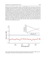
It is clear from Fig.4 that (x)H

is larger where
(x)
φ
is small, and vice versa. When 0x → ,
()Hx

reaches a maximum, while
φ
approaches to zero. On the other hand, when x →∞,
φ

becomes very large, while
()Hx

approaches to zero. This shows that the system is still in
superconductive state.These are exactly the well-known behaviors of vortex lines-magnetic
flux lines in type-II superconductors [66-67]. Thus we explained clearly the macroscopic
quantum effect in type-II superconductors using GL equation of motion of superconductive
electron under action of an electromagnetic-field.

Fig. 3. The effective potential energy in Eq. (67).


Fig. 4. Changes of φ(x) and
(x)H

with x in Eqs. (67)-(68)
Properties of Macroscopic Quantum Effects
and Dynamic Natures of Electrons in Superconductors

195
Recently, Garadoc-Daries et al. [68], Matthews et al. [69] and Madison et al.[70] observed
vertex solitons in the Boson-Einstein condensates. Tonomure [71] observed experimentally
magnetic vortexes in superconductors. These vortex lines in the type-II-superconductors are
quantized. The macroscopic quantum effects are well described by the nonlinear theory
discussed above, demonstrating the correctness of the theory.
We now proceed to determine the energy of the soliton given by (67). From the earlier
discussion, the energy of the soliton is given by:
22
22
+
224 2
00
0
22
0
2
1b
=() 1(1)

224 322
22
b
db B b B
Edx
dx
∞
−∞


ϕϕ
ϕ
+ϕ−ϕ− ≈ϕ −+ − −


ϕϕ






which depends on the interaction between superconductive electrons and electromagnetic
field.
From the above discussion, we understand that for a bulk superconductor, the
superconductive electrons behave as solitons, regardless of the presence of external fields.
Thus, the superconductive electrons are a special type of soliton. Obviously, the solitons are
formed due to the fact that the nonlinear interaction
2
λ

φφ
suppresses the dispersive effect
of the kinetic energy in Eqs. (52) and (53). They move in the form of solitary wave in the
superconducting state. In the presence of external electromagnetic fields, we demonstrate
theoretically that a permanent superconductive current is established and that the vortex
lines or magnetic flux lines also occur in type-II superconductors.
5. The dynamic properties of electrons in superconductive junctions and its
relation to macroscopic quantum effects
5.1 The features of motion of electron in S-N junction and proximity effect
The superconductive junction consists of a superconductor (S) which contacts with a normal
conductor (N), in which the latter can be superconductive. This phenomenon refers to a
proximity effect. This is obviously the result of long- range coherent property of
superconductive electrons. It can be regarded as the penetration of electron pairs from the
superconductor into the normal conductor or a result of diffraction and transmission of
superconductive electron wave. In this phenomenon superconductive electrons can occur in
the normal conductor, but their amplitudes are much small compare to that in the
superconductive region, thus the nonlinear term
2
λ
φφ
in GL equations (53)-(54) can be
neglected. Because of these, GL equations in the normal and superconductive regions have
different forms. On the S side of the S-N junction, the GL equation is [72]

2*
3
ie
(A) 20
2m ch
∇−

φ
−α
φ
+λ
φ
=



(69)
while that on the N side of the junction is

2*
ie
(A)'0
2m ch
∇−
φ
−α
φ
=



(70)
Thus, the expression for J

remains the same on both sides.

Superconductivity – Theory and Applications

196

*2
2
**
e(e*)
J( ) A
2mi mc
= φ ∇φ − φ∇φ − φ



(71)
In the S region, we have obtained solution of (69) in the previous section, and it is given by
(65) or (67) and (68). In the N region, from Eqs. (70)- (71) we can easily obtain

'
2'22 '
'
2222i '2 2 'i2 2i2
N0 0
1
() 4dsin(2bx)
22
1
e()4dsin(2bx)e e
22
−θ −θ −θ


ε
ϕ=ε− +



ε

φ=ϕφ = ε − + φ




(72)
where
'
'
2'2
2m 1
b,
α
==
ξ


2
2
22
4J m
2d ,
(e*) '

λ
=
α



'
''
b
E.
2
=ε .
here 'ε is an integral constant. A graph of
φ
vs. x in both the S and the N regions, as shown
in Fig.5, coincides with that obtained by Blackbunu [73]. The solution given in Eq. (72) is the
analytical solution in this case. On the other hand, Blackbunu’s result was obtained by
expressing the solution in terms of elliptic integrals and then integrating numerically. From
this, we see that the proximity effect is caused by diffraction or transmission of the
superconductive electrons
5.2 The Josephson effect in S-I-S and S-N-S as well as S-I-N-S junctions
A superconductor-normal conductor -superconductor junction (S-N-S) or a superconductor-
insulator-superconductor junction (S-I-S) consists of a normal conductor or an insulator
sandwiched between two superconductors as is schematically shown in Fig.6a
．The
thickness of the normal conductor or the insulator layer is assumed to be L and we choose
the z coordinate such that the normal conductor or the insulator layer is located
at
L/2 x L/2−≤≤
. The features of S-I-S junctions were studied by Jacobson et al.[74]. We

will treat this problem using the above idea and method [75-76].
The electrons in the superconducting regions (
xL/2≥ ) are depicted by GL equation (69).
Its’ solution was given earlier in Eq.(67). After eliminating u
1
from Eq.(66), we have [73-74]
00
1
J= e * u (1 )u
2m
α
α−
λ
.


Fig. 5. Proximity effect in S-N junction
Properties of Macroscopic Quantum Effects
and Dynamic Natures of Electrons in Superconductors

197

Fig. 6. Superconductive junction of S-N(I)-S and S-N-I-S
The electrons in the superconducting regions (
xL/2≥ ) are depicted by GL equation (69). Its’
solution was given earlier. Setting
0
J/ u 0dd = , we get the maximum current
c
e*

J
33m
αα
=
λ
.
This is the critical current of a perfect superconductor, corresponding to the three-fold
degenerate solution of Eq.(66), i.e.,u
1
=u
0
.
From Eq.(71), we have
222
0
mJc hc
A
e*
(e*)
=− + ∇θ
φϕ



. Using the London gauge,
.A 0∇=

, we can
get[75-76]
2

222
0
mJ 1
()
e*
dd
dx
dx
θ
=
φϕ

.
Integrating the above equation twice , we get the change
of the phase to be

222
0
mJ 1 1
()
e*
dx
∞
Δθ = −
φϕϕ


(73)
where
2

u
ϕ
= , and
2
0
u
∞
ϕ= . Here we have used the following de Gennes boundary
conditions in obtaining Eq. (73)

xx
0, 0, ( x )
dd
dx dx
∞
→∞ →∞
φθ
==
φ
→∞ =
φ
(74)
If we substitute Eqs.(64) - (67) into Eq.(73), the phase shift of wave function from an
arbitrary point x to infinite can be obtained directly from the above integral, and takes the
form of:

11
11
L
01 1

uu
(x ) tan tan
uu uu
−−
Δθ → ∞ = − +
−−
(75)
For the S-N-S or S-I-S junction, the superconducting regions are located at
xL/2≥
and the
phase shift in the S region is thus

Superconductivity – Theory and Applications

198

1
1
sL
s1
Lu
=2 ( ) 2 tan
2uu
−
Δθ Δθ → ∞ ≈
−
(76)
According to the results in (70) - (71) and the above similar method, the change of the phase
in the I or N region of the S-N-S or S-I-S junction may be expressed as [75-76]

'2 '
1
N
'
0
2e * h b L mJL
2 tan [ tan( )]
J8m 2
2e*h
−
α
Δθ = − +
λ
μ


(77)
where
'
N
2
'
tan( /2)
8m J
h
2e *
tan( b L /2)
Δθ
λ
=

α

,
'
0
mJL
2e*h
μ

is an additional term to satisfy the boundary
conditions (74),and may be neglected in the case being studied.
Near the critical temperature (T<Tc), the current passing through a weakly linked
superconductive junction is very small ( J 1<<

), we then have
2
2
'
1
22
4J m
2A ,
(e*)
λ
μ= =
α

and
g’=1. Since
2

η
ϕ
and
2
/ddxϕ are continuous at the boundary x=L/2, we have
sN
x L/2 x L/2
dd
dx dx
==
μμ
=
,
s s x L/2 N N x L/2==
ημ =η μ ,
where
s
η
and
N
η
are the constants related to features of superconductive and normal
phases in the junction, respectively. These give [75-76]
''
N1 s
2bAsin(2 ) [1 cos(2 )]sin(bL)Δθ = ε − Δθ ,
'
sNsN
cos( b L)sin(2 ) sin(2 ) sin(2 )Δθ = ε Δθ + Δθ + Δθ
where

1NS
/ε=η η
. From the two equations, we can get
''
sN
22mJ
sin( ) b sin( b L)
e*
λ
Δθ + Δθ =
α

.
Thus

max s N max
J=J sin( ) J sin( )Δθ + Δθ = Δθ
 
(78)
where

s
max s N
''
e*
1
J.,
22mbsin(bL)
α
=Δθ=Δθ+Δθ

λ

(79)
Equation (78) is the well-known example of the Josephson current. From Section I we know
that the Josephson effect is a macroscopic quantum effect. We have seen now that this effect
can be explained based on the nonlinear quantum theory. This again shows that the
macroscopic quantum effect is just a nonlinear quantum phenomenon.
From Eq. (79) we can see that the Josephson critical current is inversely proportional to sin
(
'
b L
), which means that the current increases suddenly whenever
'
b L
approaches to
nπ
,
Properties of Macroscopic Quantum Effects
and Dynamic Natures of Electrons in Superconductors

199
suggesting some resonant phenomena occurs in the system． This has not been observed
before. Moreover
max
J

is proportional to
'
s
e* /2 2m bαλ=

SN
(e* /4m )αλα , which is
related to (T-T
c
)
2
．
Finally, it is worthwhile to mention that no explicit assumption was made in the above on
whether the junction is a potential well ( α <0) or a potential barrier ( α >0). The results are
thus valid and the Josephson effect in Eq. (2.78), occurs for both potential wells and for
potential barriers.
We now study Josephson effect in the superconductor -normal conductor-insulator-
superconductor junction (SNIS) is shown schematically in Fig. 6b. It can be regarded as a
multilayer junction consists of the S-N-S and S-I-S junctions. If appropriate thicknesses for
the N and I layers are used (approximately 20 °A– 30 °A), the Josephson effect similar to that
discussed above can occur in the SNIS junction. Since the derivations are similar to that in
the previous sections, we will skip much of the details and give the results in the following.
The Josephson current in the SNIS junction is still given by
max
J=J sin( )Δθ


but, where
s1 N s2I
Δθ = Δθ + Δθ + Δθ + Δθ and
'
1
max
''
2'

1
'' 22
sinh( b L)
1
J{ }
b 2[cosh( b L) cos(2 )]
1
[1 cos(2 )][1 cos(2 )] [1 cos(2 )][1 cos(2 )]
[1 cos (2 )]sinh( b L)
1
{}
b 2[cosh( b L) cos(2 )] 1 cos (2 )
1
[1 cos(2 )][1 cos(2 )]
N
NN N
NI NI
NN
NN N N
NI
ε
=×
−Δθ
−
+ Δθ + Δθ − − Δθ − Δθ
ε− Δθ
×
−Δθ−+ Δθ
−Δθ−Δθ


[1 cos(2 )][1 cos(2 )]
NI
++ Δθ + Δθ
,
It can be shown that the temperature dependence of
max
J
is
2
max 0
()
c
JTT∝− ,which is quite
similar to the results obtained by Blackburm et al[73] for the SNIS junction and those by
Romagnan et al[7] using the Pb-PbO-Sn-Pb junction. Here, we obtained the same results
using a complete different approach. This indicates again that we can obtain some results,
which agree with the experimental data.
6. The nonlinear dynamic-features of time- dependence of electrons in
superconductor
6.1 The soliton solution of motion of the superconductive electron
We studied only the properties of motion of superconductive electrons in steady states in
superconductors in section 2.3.2, and which are described by the time-independent GL
equation. In such a case, the superconductive electrons move as solitons. We ask, “What are
the features of a time-dependent motion in non-equilibrium states of a superconductor?”
Naturally, this motion should be described by the time-dependent Ginzburg-Landau
(TDGL) equation [48-54,77] in this case. Unfortunately, there are many different forms of the

Superconductivity – Theory and Applications

200

TDGL equation under different conditions. The one given in the following is commonly
used when an electromagnetic field
A


is involved

2
2
12
2()
2
ie
ie r A
tmc
∂−

−
μφ
=∇− +α
φ
−λ
φφ


∂





Γ
(80)
and

2
2
14
() ( * *)
Aie e
Jr A
ct m mc

∂
=σ − −∇
μ
+
φ
∇
φ
−
φ
∇
φ
−
φ

∂







(81)
here
1i =−,
11 4AJ
A
ct c t c

∂∂ π
∇×∇× = − −∇μ +


∂∂





and σ is the conductivity in the normal
state,
Γ
is an arbitrary constant, and
μ
is the chemical potential of the system. In practice,
Eq. (80) is simply a time-dependent Schrödinger equation with a damping effect.
In certain situations, the following forms of the TDGL equation are also used.

2

2
2
2
2
ie
iA
tm c
∂φ

=− ∇−
φ
+α
φ
−λ
φφ

∂





(82)
or

2
2
2
1'2
2()

ie
iie A
tc
∂ξ
 
−
μφ
=α−λ
φφ
+∇−
φ
 
∂
 




ΓΓ
(83)
here
'/2mξ= , and equation (82) is a nonlinear Schrödinger equation under an
electromagnetic field having soliton solutions. However, these solutions are very difficult to
find, and no analytic solutions have been obtained. An approximate solution was obtained
by Kusayanage et al [78] by neglecting the
3
φ
term in Eq. (80) or Eq. (82), in the case of
(0, ,0),AHx=



, =(0, 0, ) KEx H Hμ=−



and =( ,0,0)EE



, where H


is the magnetic field, while
E

is the electric field .We will solve the TDGL equation in the case of weak fields in the
following.
TDGL equation (83) can be written in the following form when
A


is very small[80-81]

2
2
2
-2
2
ie
tm

∂φ λ α

+∇
φ
+
φφ
=
μφ

∂



ΓΓ Γ
(84)
Where α and Γ are material dependent parameters, λ is the nonlinear coefficient, m is the
mass of the superconductive electron. Equation (84) is actually a nonlinear Schrödinger
equation in a potential field
/2eαμ
Γ−
. Cai, Bhattacharjee et al [79], and Davydov [45]
used it in their studies of superconductivity. However, this equation is also difficult to
solve
．In the following, Pang solves the equation only in the one-dimensional case.
For convenience, let
/tt
′
= 
,
2/xxm

′
= 
Γ
, then Eq. (84) becomes

2
2
2
-2 ( )iex
t
x
∂φ ∂ φ λ α


′
++
φφ
=
μφ


′
∂
′
∂


ΓΓ
(85)
Properties of Macroscopic Quantum Effects

and Dynamic Natures of Electrons in Superconductors

201
If we let
20e
α
−
μ
=
Γ
, then Eq. (85) is the usual nonlinear Schrödinger equation whose
solution is of the form [80-81]

0
(,)
0
0
(,) ,
ixt
s
xte
′′
θ
′′
φ=ϕ (86)

22
0
(2) (2)
(,) sec ( )

24
ece ece
e
xt h x t


υ − υυ υ − υυ
′′  ′′
ϕ=× −υ
λ




Γ
(87)
here
0
1
(,) ( )
2
ec
xt x t
′′ ′ ′
θ=υ−υ
. In the case of
-2 0e
α
μ
≠

Γ
, let KEx
′
μ=−

, where K is a constant,
and assume that the solution is of the form [80-81]

(,)
'( , )
ixt
xte
′′
θ
′′
φ=ϕ (88)
Substituting Eq. (88) into Eq. (86), we get:

2
2
3
2
'
'' (')2 '
()
KeEx
tt
x
∂θ ∂θ ∂ ϕ λ α
  

′
−
ϕ
−
ϕ
++
ϕ
=+
ϕ
  
′′
∂∂ ′
∂
  

ΓΓ
(89)

2
2
''
2'0
()
txx
x
∂ϕ ∂ϕ ∂θ ∂ θ
++
ϕ
=
′′′

∂∂∂
′
∂
(90)
Now let
'( , ) ( ),xt
′′
ϕ
=
ϕξ
(),xut
′′
ξ
=− ()ut
′
=
2
2()EKe t t d
′′
−+υ+

, where (')ut describes the
accelerated motion of
'( , )xt
′′
ϕ
. The boundary condition at
′
ξ
→∞ requires ()

ϕξ
to approach
zero rapidly. When 2
0u∂θ ∂
ξ
−≠

, equation (90) can be written as:
2
()
(/2)
gt
u
′
ϕ=
∂θ ∂ξ −

, or

2
()
2
gt
u
x
′
∂θ
=+
′
∂

ϕ

(91)
where / 'ududt=

. Integration of (91) yields:

2
0
''
(,) () ()
2
x
dx u
xt gt x ht
′
′′ ′ ′ ′
θ= ++
ϕ


(92)
and where
(')ht is an undetermined constant of integration. From Eq. (92) we can get:

0
222
0
''
() ()

2
x
x
gu gu
dx u
gt x ht
t
′
′
=
∂θ
′′′
=−+++
′
∂
ϕϕϕ





(93)
Substituting Eqs. (92) and (93) into Eq. (89), we have:

2
22
3
0
2223
0

''
2()
24
()
x
x
gu g
uudx
KEex x h t g
x
′
′
=


∂ϕ α λ

′′′
=++++++ϕ−ϕ+



′
∂
ϕϕ ϕ







 



ΓΓ
(94)

Superconductivity – Theory and Applications

202
Since
2
2
()x
∂
ϕ
′
∂
=
2
2
d
d
ϕ
ξ
, which is a function of
ξ
only, the right-hand side of Eq. (94) is also a
function of

ξ
only, so it is necessary that
0
() constantgt g
′
== , and
'
2
'''
2
x0
gu
uu
(2KEex + )+ x h(t )+ ( )
24
f
V
=
α
++=
ξ
Γ

 


. Next, we assume that
0
() ()VV
ξ

=
ξ
−
β
, where
β is real and arbitrary, then

2
00
2
2() ()
24
x
gu
uu
KEex V x h t
′
=

α
′′ ′
+= ξ− +β− − −

Γ
ϕ



 



(95)
Clearly in the case discussed,
0
()V
ξ
=
0, and the function in the brackets in Eq. (95) is a
function of t′. Substituting Eq. (95) into Eq. (94), we can get [80-81]:


 
2
33
2
0
2
/g
∂ϕ λ
=
βϕ
−
ϕ
+
ϕ
∂ξ
Γ
(96)
This shows that


ϕ
is the solution of Eq. (96) when
β
and g are constant. For large
ξ
, we
may assume that

1
/
+Δ
ϕ ≤β ξ
, when
Δ is a small constant. To ensure that

ϕ
and

22
ddϕξ

approach zero when
ξ
→ ∞ , only the solution corresponding to g
0
=0 in Eq. (96) is kept, and
it can be shown that this soliton solution is stable in such a case. Therefore, we choose g
0
=0
and obtain the following from Eq. (91):

//2
xu
′
∂θ ∂ =

(97)
Thus, we obtain from Eq. (95) that
2
'''
uu
2KEex + x h(t )-
24
α
=− +β−
Γ
 


,
2232
14
() ( )() ()
43

h t t KEe t e KE t
α

′′′′
=β− − υ − +υ




Γ
(98)
Substituting Eq. (98) into Eqs. (92) - (93), we obtain:

2232
114
2()()()
243
KEet x t KEe t e KE t
α

′′ ′ ′ ′
θ= − + υ + β− − υ − + υ



Γ
(99)
Finally, substituting the Eq. (99) into Eq. (96), we can get


 
2
3
2
0
∂ϕ λ

−
βϕ
+
ϕ
=
∂ξ
Γ
(100)
When 0
β
> , the solution of. Eq. (100) is of the form


()
2
sec
h
β
ϕ
=
βξ
λ
Γ
(101)
Thus [80-81]
Properties of Macroscopic Quantum Effects
and Dynamic Natures of Electrons in Superconductors

203

2
2
23 2
2
23
222
sec
22 14()
exp
24
3

meKEttd
hx
eKEt m t eKE t KeEt
ix


β−υ−
φ= β + ×



λ







−υ α υ

 
++β−−υ−+



 
 











ΓΓ
Γ
Γ
(102)
This is also a soliton solution, but its shape
，amplitude and velocity have been changed
relatively as compared to that of Eq. (87). It can be shown that Eq. (102) does indeed satisfy
Eq. (85). Thus, equation (85) has a soliton solution. It can also be shown that this solition
solution is stable.
6.2 The properties of soliton motion of the superconductive electrons

For the solution of Eq. (102), we may define a generalized time-dependent wave number,
2
2
kKEet
x
∂θ υ
′
==−
′
∂

and a frequency

222
2
1
2()()
4
22
KEex e KEe t
t
KEe t KEex k
∂θ α

′′
ω=− = −
β
−−υ+ −

′

∂

α
′′
υ= −β− +


Γ
Γ
(103)
The usual Hamilton equations for the superconductive electron (soliton) in the macroscopic
quantum systems are still valid here and can be written as [80-81]
2
k
dk
KEe
dt x
∂ω
=− =−
′′
∂

,
then the group velocity of the superconductive electron is

22 4
2
gx
dx
KEet KEet

dt k
′
′
∂ω υ

′′
υ= = = − =υ−

′
∂


(104)
This means that the frequency ω still represents the meaning of Hamiltonian in the case of
nonlinear quantum systems. Hence,
0
xk
dd dk dx
dt dk dt x dt
′
′
ωω ∂ω
=+=
′′′′
∂
, as seen in the usual
stationary linear medium.
These relations in Eqs. (103)-(104) show that the superconductive electrons move as if they
were classical particles moving with a constant acceleration in the invariant electric-field,
and that the acceleration is given by

4KEe−

. If υ >0, the soliton initially travels toward the
overdense region, it then suffers a deceleration and its velocity changes sign. The soliton is
then reflected and accelerated toward the underdense region.The penetration distance into
the overdense region depends on the initial velocity
υ .
From the above studies we see that the time-dependent motion of superconductive electrons
still behaves like a soliton in non-equilibrium state of superconductor. Therefore, we can
conclude that the electrons in the superconductors are essentially a soliton in both time-
independent steady state and time-dependent dynamic state systems. This means that the
soliton motion of the superconductive electrons causes the superconductivity of material.
Then the superconductors have a complete conductivity and nonresistance property

Superconductivity – Theory and Applications

204
because the solitons can move over a macroscopic distances retaining its amplitude,
velocity, energy and other quasi- particle features. In such a case the motions of the
electrons in the superconductors are described by a nonlinear Schrödinger equations (52),
or (53) or (80) or (82) or (84). According to the soliton theory, the electrons in the
superconductors are localized and have a wave-corpuscle duality due to the nonlinear
interaction, which is completely different from those in the quantum mechanics.
Therefore, the electrons in superconductors should be described in nonlinear quantum
mechanics[16-17].
7. The transmission features of magnetic-flux lines in the Josephson
junctions
7.1 The transmission equation of magnetic-flux lines
We have learned that in a homogeneous bulk superconductor, the phase ( , )rt
θ


of the
electron wave function
() ()
()
,
,,
irt
rt f rte
θ
φ
=



is constant, independent of position and time.
However, in an inhomogeneous superconductor such as a superconductive junction
discussed above,
θ
becomes dependent of
r

and t. In the previous section, we discussed
the Josephson effects in the S-N-S or S-I-S, and SNIS junctions starting from the
Hamiltonican and the Ginzburg-Landau equations satisfied by
()
,rt
φ

, and showed that the

Josephson current, whether dc or ac, is a function of the phase change,
12
ϕ
θθ θ
=Δ = − . The
dependence of the Josephson current on
ϕ
is clearly seen in Eq. (78) . This clearly indicates
that the Josephson current is caused by the phase change of the superconductive electrons.
Josephson himself derived the equations satisfied by the phase difference
ϕ
, known as the
Josephson relations, through his studies on both the dc and ac Josephson effects. The
Josephson relations for the Josephson effects in superconductor junctions can be
summarized as the following,

sin ,
sm
JJ=
ϕ

2eV
t
∂ϕ
=
∂

,
2' /
y

ed H c
x
∂ϕ
=
∂

, 2' /
x
ed H c
y
∂ϕ
=
∂
 (105)
where d’ is the thickness of the junction. Because the voltage V and magnetic field
H

are
not determined, equation (105) is not a set of complete equations. Generally, these equations
are solved simultaneously with the Maxwell equation (4 / )
HcJ∇× = π


. Assuming that the
magnetic field is applied in the xy plane, i.e.
(,,0)
xy
HHH=



, the above Maxwell equation
becomes

4
( , ,) (, ,) ( , ,)
yx
H xyt H xyt Jxyt
xyc
∂∂ π
−=
∂∂
(106)
In this case, the total current in the junction is given by
0
(,,) (,,) (,,)
snd
J J xyt J xyt J xyt J=+++
In the above equation,
(,,)
s
Jxytis the superconductive current density, (,,)
n
Jxytis the
normal current density in the junction (J
n
=V/R(V ) if the resistance in the junction is R(V )
and a voltage V is applied at two ends of the junction),
(,,)
d
Jxyt is called a displacement

current and it is given by
()/
d
JCdVtdt= , where C is the capacity of the junction, and
0
J is a
constant current density. Solving the equations in Eqs,(102) and (106) simultaneously, we
can get
Properties of Macroscopic Quantum Effects
and Dynamic Natures of Electrons in Superconductors

205

2
2
2
00
22
0
11
()sin
J
I
t
v
t
∂ϕ ∂ϕ
∇
ϕ
−−

γ
=
ϕ
+
∂
λ
∂
(107)
where
2
00
/4 ', 1/ ,vc Cd RC=πγ=
22
00
/4 ' *, 4 * / , * 2
J
cdeIeJceeλ= π = π =.
Equation (107) is the equation satisfied by the phase difference. It is a Sine-Gordon equation
(SGE) with a dissipative term. From Eq.(105), we see that the phase difference
ϕ
depends on
the external magnetic field
H


, thus the magnetic flux in the junction
'
*
c
Hds A dl dl

c
Φ= = =
ϕ
 
 



can be specified in terms of
ϕ
, where
A


is vector potential of
electromagnetic field,
dl

is line element of vortex lines. Equation (107) represents
transmission of superconductive vortex lines. It is a nonlinear equation. Therefore, we know
clearly that the Josephson effect and the related transmission of the vortex line, or magnetic
flux, along the junctions are also nonlinear problems. The Sine-Gordon equation given
above has been extensively studied by many scientists including Kivshar and Malomed[39-
40]. We will solve it here using different approaches.
7.2 The transmission features of magnetic-flux lines
Assuming that the resistance R in the junction is very high, so that 0
n
J → , or equivivalently
0
0

γ
→ , setting also I
0
= 0, equation (107) reduces to

2
2
2
22
0
11
sin
J
v
t
∂ϕ
∇
ϕ
−=
ϕ
λ
∂
(108)
Define
0
/, /
J
J
Xx Tvt=λ= λ , then in one-dimension, the above equation becomes
22

22
sin
XT
∂ϕ ∂ϕ
−=
ϕ
∂∂

which is the 1D Sine-Gordon equation. If we further assume that
(,) (')XT
ϕ
=
ϕ
=
ϕ
θ with
'
000
'' ','/ /2,'/2/X X vT X X hc LI e T T I e hcθ= − − = =
it becomes
22
'
(1 ) ( ') 2( ' cos )vA
θ
−
ϕ
θ= −
ϕ
,where A’ is a constant of integration. Thus
0

(')
1/2
[( ' cos )] 2 'Ad
ϕθ
−
ϕ
−
ϕϕ
=δνθ


where
2
1/ 1 , 1v
ν
=−δ=±. Choosing A’=1, we have
1/2
(')
[sin( /2)] 2 'd
−
ϕθ
π
ϕϕ
=νθ


A kink soliton solution can be obtained as follows
' ln[tan( /2)],±νθ =
ϕ
'or

1
(') 4tan [exp( ')]
−
ϕ
θ= ±νθ . Thus yields

1'
0
(',')4tan{exp[(' ')]}XT X X vT
−
ϕ=δν−−
(109)

Superconductivity – Theory and Applications

206
From the Josephson relations, the electric potential difference across the junction can be
written as
'
00
0
2
2
2sec[('')]
2'2 ' 2
o
Ie
dd
VvhXXvT
edT c dT c

c
ϕϕ
ϕϕ
== =δν ν−−
ππ



where
72
0
210 /cGausscm
−−
ϕ =π = × 'is a quantum fluxon, c is the speed of light. A similar
expression can be derived for the magnetic field
'
00
0
2
2
2sec[('')]
2'2 ' 2
o
z
Ie
dd
HhXXvT
edX c dX c
c
ϕϕ

ϕϕ
== =±δν ν−−
ππ



We can then determine the magnetic flux through a junction with a length of L and a cross
section of 1 cm2. The result is
'
00
'(,) (',')'
xx
Hxtdx B HXTdX
∞∞
−∞ −∞
Φ= = =δ
ϕ


Therefore, the kink ( 1δ=+ ) carries a single quantum of magnetic flux in the extended
Josephson junction. Such an excitation is often called a fluxon, and the Sine-Gordon
equation or Eq.(107) is often referred to as transmission equation of quantum flux or fluxon.
The excitation corresponding to δ = −1 is called an antifluxon. Fluxon is an extremely stable
formation. However, it can be easily controlled with the help of external effects. It may be
used as a basic unit of information.
This result shows clearly that magnetic flux in superconductors is quantized and this is a
macroscopic quantum effect as mentioned in Section 1. The transmission of the quantum
magnetic flux through the superconductive junctions is described by the above nonlinear
dynamic equation (107) or (108).The energy of the soliton can be determined and it is given by
2

8/,Em=
β
where
22
/1/
J
m
β
=λ.
However, the boundary conditions must be considered for real superconductors. Various
boundary conditions have been considered and studied. For example, we can assume the
following boundary conditions for a 1D superconductor,
(0, ) ( , ) 0
xx
tLt
ϕ
=
ϕ
= . Lamb[47]
obtained the following soliton solution for the SG equation (108)

1
(,) 4tan [()()]xt hx
g
t
−
ϕ=
(110)
where h and g are the general Jacobian elliptical functions and satisfy the following
equations

24 2
[()] ' (1 ') ',hx ah b h c=++ −
242
[()] ' ' '
g
xchbha=+−
with a’, b’, and c’ being arbitrary constants. Coustabile et al. also gave the plasma oscillation,
breathing oscillation and vortex line oscillation solutions for the SG equation under certain
boundary conditions. All of these can be regarded as the soliton solution under the given
conditions.
Solutions of Eq.(108) in two and three-dimensional cases can also be found[80-81]. In two-
dimensional case, the solution is given by
Properties of Macroscopic Quantum Effects
and Dynamic Natures of Electrons in Superconductors

207

1
(,,)
(,,) 4tan[ ]
(,,)
g
XYT
XYT
f
XYT
−
ϕ= (111)
where
0

/, /, /
J
JJ
Xx Yy Tvt=λ=λ= λ,
12 23 13
1(1,2) (2,3) (3,1)
yy yy yy
fae aeae
+++
=+ = ,
12 123
(1,2) (2,3) (3,1)
yy yyy
ge e a a a e
++
=++
and
02 2 2
1
, 1,( 1,2,3)
ii iiiii
ypXqY ypq i=+−Ωτ− +−Ω==
22 2
22 2
()()( )
(, ) ,(1 3)
()()( )
ij ij i j
ij ij i j
pp qq

ai j i j
pp qq
−+−+Ω−Ω
=≤≤≤
++++Ω+Ω

In addition, P
i
, q
i
and
i
Ω satisfy
11 1
22 2
33
det 0
3
pq
pq
pq
Ω
Ω=
Ω
. In the three-dimensional case, the
solution is given by

1
(,,,)
(,,,) 4tan[ ],

(,,,)
g
XYZT
XYZT
f
XYZT
−
ϕ= , (112)
where X, Y , and T are similarly defined as in the 2D case given above, and /
J
Zz=λ . The
functions f and g are defined as
12 23 13
233
1
yy yy yy
fdXe dYe dZe
+++
=+++,
123 123
233
yyy yyy
g e e e dX dY dZ e
++
=+++ ,
2222
123 123
,1,(,,)
ii i i i ii i i i
y

aX aY a bT C a a a b i XYZ=+++− ++−==
with
3
22
1
3
22
[( ) ( ) ]
(, ) ,(1 3),
[( ) ( ) ]
ik jk i j
k
ik jk i j
k
aa bb
di j j
aa bb
=
−−−
=≤≤
+−+



here
3
y
is a linear combination of
1
y

and
2
y
, i.e.,
312
y
yy=α +
β
.
We now discuss the SG equation with a dissipative term
0
/ t
γ
∂
ϕ
∂
. First we make the
following substitutions to simplify the equation
22
0000
/, / /, /,' .
J
JJ J J
Xx Tvt t a vB I=λ= λ=ω=
γ
λ=λ
In terms of these new parameters, the 1D SG equation (107) can be rewritten as

2
22

2
sin 'aB
T
X
T
∂ϕ ∂ϕ ∂ϕ
−−=
ϕ
+
∂
∂
∂
(113)
The analytical solution of Eq.(113) is not easily found. Now let

Superconductivity – Theory and Applications

208

2
000
22
2
0
0
0
1
1
,,','
1

vXvTav
q
av
av
v
−−
α= η= =
ϕ
=π+
ϕ
α
−
(114)
Equation (113) then becomes

2
2
'sin'0qB
∂ϕ ∂ϕ
++
ϕ
−=
∂η
∂η
(115)
This equation is the same as that of a pendulum being driven by a constant external moment
and a frictional force which is proportional to the angular displacement. The solution of the
latter is well known, generally there exists an stable soliton solution[80-81]. Let
'/Yd d=ϕ η
,

equation (115) can be written as

'sin''0
Y
qY B
∂
++
ϕ
−=
∂η
(116)
For 0 ' 1B<<, we can let
00
'sin (0 /2)B =
ϕ
<
ϕ
<π and
01
'
ϕ
=−π−
ϕ
+
ϕ
, then, equation (116)
becomes

010
'sin sin( )

Y
YqY
∂
=− +
ϕ
+
ϕ
−
ϕ
∂η
(117)
Expand Y as a power series of
1
ϕ
, i.e.,
1
,
n
n
n
Yc=
ϕ

and inserting it into Eq.(117), and
comparing coefficients of terms of the same power of
1
ϕ
on both sides, we get

2

0
102
1
''
sin1
cos ,
24 '32
qq
cc
qc
ϕ
=− ± + ϕ =−
+
,
2
00
32423
11
cos sin
11
(2 ), (5 )
'4 6 '5 24
ccccc
qc qc
ϕϕ
=−− =−−
++
(118)
and so on. Substituting these
'

n
cs into
2
1
'/ ,
n
n
Yd d c=
ϕ
η=
ϕ

the solution of
1
ϕ
may be
found by integrating
2
11
/
n
n
dc
η
=
ϕϕ


. In general, this equation has soliton solution or
elliptical wave solution. For example, when

23
11 21 31
'/ddc c cϕ η= ϕ + ϕ + ϕ
it can be found that
1
1
2
(,sin( ))
AB A
F
AC AB
AC
−
−−ϕ
η=
−−
−

where
1
(, )Fk
ϕ
is the first Legendre elliptical integral, and A, B and C are constants. The
inverse function
1
ϕ
of
1
(, )Fk
ϕ

is the Jacobian amplitude '
1
amFϕ=
. Thus,
1
1
sin ( )
AAC
am
AB AB
−
−ϕ −
=η
−−
or
1
)( )
AAC
sn
AB AB
−ϕ −
=η
−−

where snF is the Jacobian sine function. Introducing the symbol cscF = 1/snF, the solution
can be written as

2
1
( )[csc( )]

AC
AAB
AB
−
ϕ
=− − η
−
(119)
Properties of Macroscopic Quantum Effects
and Dynamic Natures of Electrons in Superconductors

209
This is a elliptic function. It can be shown that the corresponding solution at η→∞ is a
solitary wave.
It can be seen from the above discussion that the quantum magnetic flux lines (vortex lines)
move along a superconductive junction in the form of solitons. The transmission velocity
0
v
can be obtained from
2
00
1hv v=α − and
n
c in Eq. (118) and it is given by
2
00
1/ 1 [ / ( )]vh=+αϕ.
That is, the transmission velocity of the vortex lines depends on the current
0
I injected and

the characteristic decaying constant α of the Josephson junction. When α is finite, the
greater the injection current I
0
is, the faster the transmission velocity will be; and when I
0
is
finite, the greater the α is, the smaller the
0
v will be, which are realistic.
8. Conclusions
We here first reviewed the properties of superconductivity and macroscopic quantum
effects, which are different from the microscopic quantum effects, obtained from some
experiments. The macroscopic quantum effects occurred on the macroscopic scale are
caused by the collective motions of microscopic particles , such as electrons in
superconductors, after the symmetry of the system is broken due to nonlinear interactions.
Such interactions result in Bose condensation and self-coherence of particles in these
systems. Meanwhile, we also studied the properties of motion of superconductive electrons,
and arrived at the soliton solutions of time-independent and time-dependent Ginzburg-
Landau equation in superconductor, which are, in essence, a kind of nonlinear Schrödinger
equation. These solitons, with wave-corpuscle duality, are due to the nonlinear interactions
arising from the electron-phonon interaction in superconductors, in which the nonlinear
interaction suppresses the dispersive effect of the kinetic energy in these dynamic equations,
thus a soliton states of the superconductive electrons, which can move over a macroscopic
distances retaining the energy, momuntum and other quasiparticle properties in the
systems, are formed. Meanwhile, we used these dynamic equations and their soliton
solutions to obtain, and explain, these macroscopic quantum effects and superconductivity
of the systems. Effects such as quantization of magnetic flux in superconductors and the
Josephson effect of superconductivity junctions,thus we concluded that the
superconductivity and macroscopic quantum effects are a kind of nonlinear quantum effects
and arise from the soliton motions of superconductive electrons. This shows clearly that

studying the essences of macroscopic quantum effects and properties of motion of
microscopic particles in the superconductors has important significance of physics.
9. References
[1] Parks, R. D., Superconductivity, Marcel. Dekker, 1969.
[2] Rogovin, D. and M. Scully, Superconductiviand macroscopic quantum phenomena,
Phys. Rep. 25(1976) 178.
[3] Rogovin, D., Electrodynamics of Josephson junctions
，Phys. Rev. B11 (1975) 1906-108
[4] Abrikosov, A. A. and L. P. Gorkov, I.V. Dzyaloshinkii, Quantum field theoretical
mothods in statistic phyics, Pregamon Press, Oxfordea, 1965
[5] Rogovin, D., Josephson tunneling: An example of steady-state superradiance,Phys. Rev.
B12 (1975) 130-133.

Superconductivity – Theory and Applications

210
[6] Ginzburg V L, Superconductivity, Superdiamagnetism, Superfluidity , Moscow: MIR
Publ., 1987
[7] Ginzburg V L, Superconductivity, Moscow-Leningrad: Izd. Moscoew, AN SSSR, 1946
[8] Ginzburg, V. L Superconductivity and superfluidity Phys Usp. 40 (1997 ) 407
[9] Leggett, A. J., Macroscopic Effect of P- and T-Nonconserving Interactions in
Ferroelectrics: A Possible Experiment? Phys. Rev. Lett. 41 (1978) 586
[10] Leggett, A. J., in Percolation, Localization and Superconductivity, eds. by A. M.
Goldlinan,S. A. Bvilf, Plenum Press, New York, 1984. pp. 1- 41.
[11] Leggett, A. J., Low temperature physics, Springer, Berlin, 1991, pp. 1-93;
[12] Pang Xiao-feng, Investigations of properties of motion of superconductive electrons in
superconductors by nonlinear quantum mechanics, J. Electronic Science and
Technology of China, 6(2)(2008)205-211
[13] Pang, Xiao-feng, macroscopic quantum effects, Chinese J. Nature, 5 (1982) 254,
[14] Pang Xiao-feng, Investigations of properties and essences of macroscopic quantum

effects in superconductors by nonlinear quantum mechanics, Nature Sciences,
2(1)(2007) 42
[15] Pang, Xiao-feng, Investigation of solutions of a time-dependent Ginzburg-Landau
equation in superconductor by nonlinear quantumtheory, IEEE Compendex, 2009,
274-277, DOI: 10.1109/ ASEMD.2009.5306641(EI)
[16] Pang, Xiao-feng, Theory of Nonlinear Quantum Mechanics, Chongqing Press,
Chongqing, 1994.p35-97
[17] Pang Xiao-feng Nonlinear Quantum Mechanics, Beijing, Chinese Electronic Industry
Press, Beijing, 2009,p20-63
[18] Bardeen, L. N., L. N. Cooper and J. R. Schrieffer, Superconductivity theory, Phys. Rev.
108 (1957) 1175;
[19] Cooper, L. N., The bound electronic pairs in degenerated Fermi gas Phys. Rev. 104
(1956) 1189.
[20] Schrieffer, J. R., Superconductivity, Benjamin, New York, 1969.
[21] Schrieffer, J. R., Theory of Superconductivity, Benjamin, New York, 1964.
[22] Frohlich.H., Theory of superconductive states, Phys. Rev.79(1950)845;
[23] Frohlich.H., On superconductivity theory : one-dimensional case, Proc. Roy.Soc.A,
223(1954)296
[24] Josephson, B.D, Possible New Effects in Superconducting Tunnelling , Phys. Lett. 1
(1962) 251
[25] Josephson, B.D, Supercurrents through barriers, Adv. Phys. 14 (1965) 419.
[26] Josephson, B.D., Thesis, unpublised, Cambridge University (1964)
[27] Pang, Xiao-feng, The relation between the physical parameters and effective spectrum
of phonon, Southwest Inst. For Nationalities, . 17 (1991) 1.
[28] Pang, Xiao-feng, On the solutions of the time-dependent Ginzburg-Landau equations
for a superconductor in a weak field, J. Low Temp. Physics, 58(1985)333
[29] Pang, Xiao-feng, The isotope effects of superconductor, Chinese. J. Low Temp.
Supercond.,No. 3 (1982) 62
[30] Pang, Xiao-feng, The properties of soliton motion for superconductivity electrons. Proc.
ICNP, Shanghai, 1989, p139.

[31] Rayfield, G. W. and F. Reif, Evidence for the creation and motion of quantized vortex
rings in superfluid helium, Phys. Rev. Lett. 11 (1963) 305.
[32] Perring, J. K., and T.H.R.Skyrme, A model unified field equation,Nucl. Phys. 31 (1962)
550.
Properties of Macroscopic Quantum Effects
and Dynamic Natures of Electrons in Superconductors

211
[33] Barenghi, C. F., R. J. Donnerlly and W. F.Vinen, Quantized Vortex Dynamics and
Superfluid Turbulence, Springer, Berlin, 2001.
[34] Bogoliubov, N. N., Quantum statistics, Nauka, Moscow, 1949
[35] Bogoliubov, N. N., V. V. Toimachev and D. V. Shirkov, A New Method in the Theory of
Superconductivity, AN SSSR, Moscow, 1958.
[36] London, F., superfluids Vol.1, Weley, New York 1950.
[37] de Gennes, P. G., Superconductivity of Metals and Alloys, W. A. Benjamin, New York,
1966.
[38] Suint-James, D., et al., Type-II Superconductivity, Pergamon, Oxford, 1966.
[39] Kivshar, Yu. S. and B. A. Malomed, Dynamics of solitons in nearly integrable
systems
，Rev. Mod. Phys. 61 (1989) 763.
[40] Kivshar, Yu. S., T. J. Alexander and S. K. Turitsy, Nonlinear modes of a macroscopic
quantum oscillator
， Phys. Lett. A 278(2001) 225.
[41] Bullough, R. K., N. M. Bogolyubov, V. S. Kapitonov, C. Malyshev, J. Timonen, A. V.
J.Rybin, A.V., Vazugin, G.G. and Lindberg, M, Quantum integrable and
nonintegrable nonlinear Schrodinger models for realizable Bose-Einstein
condensation in d+1 dimensions (d=1,2,3)
， Theor. Math.Phys. 134(2003)47
[42] Bullough, R. K. and P. T. Caudeey, Solitons, Plenum Press, New York, 1980.
[43] Huepe, C. and M. E. Brachet, Scaling laws for vortical nucleation solutions in a model of

superflow
，
Physica D 140 (2000) 126.
[44] Sonin, E. B., Nucleation and creep of vortices in superfluids and clean
superconductors,Physica
，B210（1995）234-250
[45] Davydov.A.S. and V.N.Ermakov, Stability of a Superconducting Condensate of
Bisolitons, Phys. Stat.Sol.B148(1988)305
[46] Landau, L. D. and E. M. Lifshitz, Quantum mechanics, Pergamon Press, Oxford, 1987
[47] Lamb, G. L., Analytical descriptions of ultrashort optical pulse propagation in a
resonant medium
，Rev. Mod. Phys. 43 (1971) 99.
[48] Ginzberg, V. L. and L. D. Landau, On the theory of superconductivity
，Zh. Eksp.
Theor. Fiz. 20 (1950) 1064;
[49] Ginzburg V.L., On superconductivity and superfluidity, Physics –Usp. 47 (2004) 1155 -
1170
[50] Ginzberg, V. L. and D. A. Kirahnits, Problems in High-Temperature Superconductivity,
Nauka, Moscow, 1977.
[51] Gorkov, L. P., On the energy spectrum of superconductors, Sov. Phys. JETP 7(1958) 505.
[52] Gorkov, L. P., Microscopic derivation of the Ginzburg-Landau equation in the theory of
superconductivity, Sov. Phys. JETP 9 (1959) 1364.
[53] Abrikosov, A. A., On the magnetic properties of superconductors of the second
group
，Zh. Eksp. Theor. Fiz. 32 (1957) 1442.
[54] Abrikosov, A. A. and L. P. Gorkov, Zh. Eksp. Theor. Phys. 39 (1960) 781;
[55] Valatin. J.G. , Comments on the theory of superconductivity, Nuovo Cimento7(1958)843
[56] Liu, W. S. and X. P. Li, BCS states as squeezed fermion-pair states, European Phys. J. D2
(1998) 1.
[57] Gross, E. F.,structure of a quantized vertex in boson systems, II Nuovo Cimento, 20

(1961) 454.
[58] Pitaevskii, L. P Vortex lines in an imperfect Bose gas. Sov. Phys. JETP-USSR, 13 (1961)451
[59] Pitaevskii, L. P. and Stringari, S. Bose–Einstein Condensation. Oxford, Clarendon Press, 2003

Superconductivity – Theory and Applications

212
[60] Elyutin P. V. and A. N. Rogovenko, Stimulated transitions between the self-trapped
states of the nonlinear Schrödinger equation, Phys. Rev. E63 (2001) 026610.
[61] Elyutin, P. V., Buryak A V, Gubernov V V, Sammut R A and Towers I N, Interaction of
two one-dimensional Bose-Einstein solitons: Chaos and energy exchange, Phys.
Rev. E64 (2001) 016607.
[62] Pang, Xiao-feng, The properties of motion of superconductive electrons in
superconductor, J. XinJiang Univ. (nature) 5(1988)33
[63] Pang Xiao-feng, The G-L theory of superconductivity bin magnetic-superconductor,
Investigations of metal materials, 12(1986) 31
[64] Perez-Garcia, V. M., M. Michinel and H. Herrero, Bose-Einstein solitons in highly
asymmetric traps, Phys. Rev. A57 (1998) 3837.
[65] London, F. and H. London, The electromagnetic equations of the superconductor, Proc.
Roy. Soc. (London) A 149 (1935) 71
[66] Pang, Xiao-feng, Interpretation of proximity effect in superconductive junctions by G-L
theory, J. Kunming Tech. Sci. Univ., 14. (1989) 78
[67] Pang, Xiao-feng, Properties of transmission of vortex lines along the superconductive
junctions. J. Kunming Tech. Sci. Univ., 14 (1989) 83.
[68] Caradoc-Davies, B. M., R. J. Ballagh and K. Bumett, Coherent Dynamics of Vortex
Formation in Trapped Bose-Einstein Condensates, Phys. Rev. Lett. 83 (1999) 895.
[69] Matthews, M. R., B. P. Anderson
*
, P. C. Haljan, D. S. Hall
†

, C. E. Wieman, and E. A.
Cornell, Vortices in a Bose-Einstein Condensate, Phys. Rev. Lett. 83 (1999) 2498.
[70] Madison, K. W., F. Chevy, W. Wohlleben, and J. Dalibard , Vortex formation in a stirred
Bose-Einstein condensate, Phys. Rev. Lett. 84 (2000) 806.
[71] Tonomura A, Kasai H, Kamimura O, Matsuda T, Harada K, Yoshida T, Akashi T,
Shimoyama J, Kishio K, Hanaguri T, Kitazawa K, Masui T, Tajima S, Koshizuka N,
Gammel PL, Bishop D, Sasase M, Okayasu S, Observation of structures of chain
vortices inside anisotropic high- Tc superconductors, Phys. Rev. Lett. 88( 2002) 237001
[72] Pang, Xiao-feng, Investigation of solutions of Josephson equation in three dimension
superconductive junctions, J. Chinghai Normal Univ. Sin. No. 1 (1989) 37.
[73] Blackbunu, J. A., H.J.T. Smith and N.L. Rowell, Proximity effects and the generalized
Ginzburg-Landau equation, Phys. Rev. B11 (1975) 1053.
[74] Jacobson, D. A., Ginzburg-Landau equations and the Josephson effect, Phys. Rev. B8
(1965) 1066;
[75] Pang, Xiao-feng, The Bose condensation properties of superconductive states, J. Science
Exploration Sin. 1(4 )(1986) 70.
[76] Pang, Xiao-feng, The features of coherent state of superconductive states, J. Southwest
Inst. For Nationalities Sin. 17 (1991) 18.
[77] Dewitt, B. S., Superconductors and Gravitational Drag, Phys. Rev. Lett. 16 (1966) 1092
[78] Kusayanage.E, T. Kawashima and K.Yamafuji,Flux flow in nonideal type-II
superconductor, J. Phys. Soc. Japan 33 (1972) 551.
[79] Cai, S. Y. and A. Bhattacharjee, Ginzburg-Landau equation: A nonlinear model for the
radiation field of a free-electron laser, Phys. Rev. A43 (1991) 6934.
[80] Pang, Xiao-feng, Soliton Physics, Press of Sichuan Sci. and Tech., Chengdu, 2003
[81] Guo Bai-lin and Pang Xiao-feng, solitons, Chinese Science Press, Beijing, 1987
0
FFLO and Vortex States in Superconductors With
Strong Paramagnetic Effect
M. Ichioka, K.M. Suzuki, Y. Tsutsumi and K. Machida
Department of Physics, Okayama University

Japan
1. Introduction
In type-II superconductors (Fetter & Hohenberg, 1969), magnetic fields penetrate into
superconductors as quantized flux lines with flux quanta φ
0
= hc/2e, where h is Planck
constant, c velocity of light, e electron’s charge. Around a flux line, pair potential ∆
(r) of
Cooper pair has a vortex structure, where ∆
(r) has phase winding 2π reflecting screening
super-current around a flux line. At the vortex core, amplitude
|∆(r)| is suppressed, and low
energy excitations appear within the superconducting gap of the electronic states.
Vortex physics makes important roles in the study of unconventional superconductors,
because unconventional characters hidden in the uniform superconducting state at a zero field
appear around vortices. For example, in superconductors with anisotropic superconducting
gap on Fermi surface in momentum space, electronic states around a vortex show real-space
anisotropy in the local density of states (LDOS) N
(E, r) around vortex core. The vortex core
image is observed by scanning tunne ling microscopy (STM) (Hess et al., 1990; Nishimori et al.,
2004). Around vortex cores, local zero-energy electronic states at Fermi level are seen as star
shape with tails extending toward node or weak-gap directions (Hayashi et al., 1996; 1997;
Ichioka et al., 1996; Schopohl & Maki, 1995). From the spatial average of the zero-energy
states, we can estimate the zero-energy density of states (DOS) N
(E = 0), which determines
low temperature (T) behaviors of physical quantities. Due to the differences of electronic
states around the vortex core, N
(E = 0) shows different magnetic field (H) dependences.
These H-dependences are studied to identify the pairing symmetry in the experiments for
vortex states, such as, electronic specific heat ( Moler et al., 1994; Nohara et al., 1999), electronic

thermal conductivity, and paramagnetic susceptibility (Zheng et al., 2002). For example, the
H-dependence of low temperature specific heat C
(H) i s often u sed to distinguish the presence
of nodes in the pairing potential. As for Sommerfeld coefficient γ
(H) ≡ lim
T→0
C(H)/T,
γ
(H) ∝ H in s-wave pairing with full gap, and γ(H) ∝
√
H by the Volovik effect in d-wave
pairing with line nodes (Ichioka et al., 1999a;b; Miranovi´c et al., 2003; Nakai et al., 2004;
Volovik, 1993). The curves of γ
(H) are expected to smoothly recover to the normal state
value towards the upper critical field H
c2
. However, in some heavy fermion superconductors,
C
(H) deviates from these curves. In CeCoIn
5
, C(H) shows convex curves, i.e., C(H) ∝ H
α
(α > 1) at higher fields(Ikeda et al., 2001). This behavior is not understood only by effects
of the pairing symmetry. A similar C
(H) behavior is observed also in UBe
13
(Ramirez et al.,
1999). The experimental data of magnetization curve M
total
(H) in CeCoIn

5
show a convex
curve at higher fields, instead of a conventional concave curve (Tayama et al., 2002). As an
10