Advanced Trends in Wireless Communications Part 6 ppt
Bạn đang xem bản rút gọn của tài liệu. Xem và tải ngay bản đầy đủ của tài liệu tại đây (499.84 KB, 35 trang )
Block Transmission Systems in Wireless Communications
165
corresponding to a single group of m signal elements, will normally be a sequence of n
g
+
non-zero sample values. The sequence of these n
g
+
values in the absence of noise is:
n
ijij
j
vby i ng
1
1, 2, ,
−
=
=
=+
∑
…
(13)
Taking a practical example to clarify the convolution here, if
m 2
=
, and g 1
=
, so n 3= and
ng4+=. The output of the channel will be the 14
×
vector V whose elements are:
[
]
ooo
b
y
b
y
b
y
b
y
b
y
b
y
b
y
b
y
b
y
b
y
b
y
b
y
1 2132112 3112213 132231−− −
=++ ++ ++ ++V (14)
Applying the limitations on the channel impulse response,
V may be written as:
[
]
ooo
b
y
bbb
y
b
y
bbb
y
b
y
bbb
y
1 23112 31213 1231
00 00 00=++ ++ ++ ++V
(15)
So, this result is multiplication of B by a 3 4
×
matrix C that depends on:
o
o
o
yy
yy
y
y
1
1
1
00
00
00
⎡
⎤
⎢
⎥
=
⎢
⎥
⎢
⎥
⎣
⎦
C
(16)
In vector form, it may be written as:
=
VBC (17)
where
V is the
(
)
n
g
1
×
+ received signal, and C is the
(
)
nn
g
×
+ channel with i
th
row is:
g
ini
og
yy y
1
1
1
00 00
+
−−
=
………
i
C (18)
Assume now that successive groups of signal-elements are transmitted, and one of these
groups is that just considered. The first transmitted impulse of the group occurs at time
T
seconds. Fig. 5 shows the
n
g
+
received samples which are the components of V.
Fig. 5. Sequence of
n
g
+
samples for one received block
Due to the Inter Block Interference (IBI), the first elements of the block (
g components) of V
are affected in part on the preceding received group of
m signal-elements. Also, the last g
components of V are dependent in part on the following received group of
m elements. Thus
…… …
ISI from
previous group
g
No ISI from
other groups
m
ISI from next
group
g
Advanced Trends in Wireless Communications
166
there is Intersymbol Interference (ISI) from adjacent received groups of elements in both the
first and the last
g components of V. However, the central m components of V depend only
on the corresponding transmitted group of
m elements, and can therefore be used for the
detection of these elements without ISI from adjacent groups.
Returning back to the same example of
m 2
=
and g 1
=
, the central m components of V are:
[
]
central o o
b
y
b
y
bbb
y
b
y
11 2 3 1 21 3
00=++ ++V (19)
which is the multiplication of B by a 3 2
×
matrix that depends on the channel, and equal to:
central
o
o
y
yy
y
1
1
0
0
⎡
⎤
⎢
⎥
=
⎢
⎥
⎢
⎥
⎣
⎦
V
B
(20)
Mathematically, if only the central
m components of V are wanted, this matrix now
represents the channel (mathematically only). To make this matrix somehow looks like the
matrix C, this matrix is the transpose of a new 2 3
×
matrix D that is equal to:
o
o
yy
yy
1
1
0
0
⎡
⎤
=
⎢
⎥
⎣
⎦
D (21)
In general, the central
m components of the vector V,
gg gm
vv v
12++ +
⎡
⎤
⎣
⎦
…
, can be
obtained by introducing a new matrix
T
BD where D is the mn
×
matrix of rank m whose i
th
row is:
g
imi
gg o
yy y
1
1
1
00 00
+
−−
−
=
………
i
D
(22)
Thus,
T
BD is a m1
×
vector where each row of it gives information about the received
symbols at that row:
gg gm
vv v
12++ +
⎡
⎤
=
⎣
⎦
…
T
BD (23)
When noise is present, the received vector is:
=+
T
RBD W (24)
It may be easily shown that the coder matrix
F has to be:
(
)
T
1−
=FDD D (25)
Thus, under the assumed conditions, the linear network
F representing the transformation
performed by the coder is such that it makes the
m signal elements of a group orthogonal at
the input of the detector and also maximizes the tolerance to additive white Gaussian noise
in the detection of these signal elements.
Now the block diagram of the precoding system, using the new assumptions about the
precoder and the channel matrix, may be re-drawn as in Fig. 6.
Block Transmission Systems in Wireless Communications
167
Fig. 6. Block diagram of the precoding system in vector form
4.3 Performance evaluation of the precoding system
Assume that the possible values of
i
s are equally likely and that the mean square value of S
is equal to the number of bits per element. Suppose that the m vectors
{
}
i
D have unit
length. Since there are m k-level signal elements in a group, the vector S has
m
k possible
values each corresponding to a different combination of the m k-level signal-elements. So,
the vector B whose components are the values of the corresponding impulses fed to the
baseband channel, has
m
k possible values. If e is the total energy of all the
m
k values of the
vector B, then in order to make the transmitted signal energy per bit equal to unity, the
transmitted signal must be divided by:
m
e
nk
= (26)
The
m samples of the received signal from which the corresponding
{
}
i
s are detected, are:
T
1
′
=+
RBDW
(27)
Then, the
m sample values which are the components of the vector V (after taking only the
central m components), must first be multiplied by the factor
to give the m vector:
T
=
=+=+RVBD WSU (28)
where
U is an m vector that represents the AWGN vector after being multiplied by .
The mean of the new noise vector
U is zero and its variance is:
T
222
η
σ
= (29)
Thus, the tolerance to noise of the system is determined by the value of
T
2
η
. When there is no
signal distortion from the channel,
(
)
T
1
−
DD
is an identity matrix. Under these conditions,
1=
, so that
T
22
η
σ
= .
Now, the block diagram can be finally drawn as:
Fig. 7. Final block diagram of the precoding system
Buffer
store
()
T
1
−
=
F
DD D
S
Data
B
C
V
R
S’
X
Buffer
store
X
1
Buffer
store
()
DDD
F
1
−
=
T
Buffer
store
S
Data
B
T
=CD
V
R
S’
Advanced Trends in Wireless Communications
168
Note that the mn× network transforms the transmitted signal such that the corresponding
sample values at the receiver are the best linear estimates of the
{
}
i
s . The variance now is
T
η
instead of
σ
. So, the bit error rate equation may be written as:
e
o
T
Perfc erfc
N
b
b
111
22
2
ξ
ξ
η
⎡⎤
⎡
⎤
==
⎢⎥
⎢
⎥
⎢
⎥
⎢⎥
⎣
⎦
⎣⎦
(30)
4.4 Numerical results of the precoding system
The bit error rate curves for the precoding system is shown in Fig. 8 (a). The signal elements
are binary antipodal having possible values as +1 or 1
−
. There are four elements in a group
(block length m 4= ) and these are equally likely to have any of the two values. The sampled
impulse response of the channel is
{
}
[
]
i
y 0.408 0.817 0.408= . This channel has a second
order null in the frequency domain and introduces severe signal (amplitude) distortion.
0 2 4 6 8 10 12 14 16
10
-7
10
-6
10
-5
10
-4
10
-3
10
-2
10
-1
10
0
Signal to Noise Ratio dB
Probability of Error Pe
BLE [50]
Proposed precoder
MSE precoder [96]
0 2 4 6 8 10 12 14 16
10
-7
10
-6
10
-5
10
-4
10
-3
10
-2
10
-1
10
0
Signal to noise ratio dB
Bit error rate
Simulation
Mathematical
Fig. 8. (a) Probability of bit error versus SNR for the precoding system,
(b) Mathematical and simulation results for the precoding system
The curves in Fig. 8 (a) were obtained by plotting the results of Eq. 30 for the proposed
precoding system, Eq. 9 for the BLE and simulating the MSE precoder. In proposed precoder
and the BLE, the same block length, and channel impulse response (CIR) were assumed. CIR
was normalized to avoid any possible bias. From Fig. 5.1, it is clear that the proposed
precoding system returns in about 2 dB enhancement in comparison with the BLE. The MSE
linear precoder is simulated using 4 transmitted antennas and 2 receivers with 8 bits per
user. The performance of the MSE precoder is better than the proposed precoder because 2
receivers are used. For high SNRs, the performance of the proposed precoder starts to be
better than the MSE precoder because the MSE precoder uses a built in estimator. This
estimator depends on pilot symbols, which will be affected by noise, and will return some
inaccuracy in the channel estimation.
The precoding system has better performance than the block linear equalizer, each one of
them provides the best linear estimate of a received group of
m signal elements. In the block
linear equalizer, all the signal processing is carried out at the receiver, while in the proposed
precoding system, all the processing is done at transmitter, and leaves the receiver simple.
Block Transmission Systems in Wireless Communications
169
The proposed system depends on transmitting the data in blocks. The source of these data
may be serial, i.e. from the same source, or even parallel from different sources. So, the
length on the block is expected to have a great effect on the performance.
Simulation program is developed by Matlab. It is assumed that the channel characteristics
are known, and fixed for all the transmission procedure. Channel impulse response may
vary through the transmission, but it must be fixed within the block, and it should be known
all the time. A certain estimation method is not suggested, but literature is rich with many
methods, and any adaptive one may be used.
In order to make a comparison between the mathematical results for the precoding system
presented in Fig. 8 (a), and the simulation program results, Fig. 8 (b) is introduced, which
clarify that the behavior is the same.
Fig. 9 (a) shows the probability of error of the system for different values of SNR using four
different lengths of the block, i.e.
m 1
=
, m 2= , m 4
=
and m 8
=
, the channel here is
assumed to have impulse response
[
]
Y 0.408 0.817 0.408= .
It is clear from the figure that increasing the block length will reduce the performance of the
system and the probability of error becomes worse. This result is expected because
increasing the block length will increase the value of the transmitted vector energy
, which
maximizes the variance of the noise
U at the output of the system as given in Eq. 29.
0 2 4 6 8 10 12 14 16
10
-60
10
-50
10
-40
10
-30
10
-20
10
-10
10
0
Signal to noise ratio dB
Bit error rate
m = 1
m = 2
m = 4
m = 8
1 2 3 4 5 6 7 8 9 10 11 12 13 14 15 16
10
-60
10
-50
10
-40
10
-30
10
-20
10
-10
10
0
Block length m
Bit error rate
Fig. 9. (a) Effect of block length on the precoding system performance,
(b) Behavior of the precoding system of different block lengths
Also, increasing the block length will increase the intersymbol interference inside the block
itself (IBI between the blocks is removed by using guard band). Theoretically, the best result
will be for
m 1= , which means transmitting each bit separately, and this is practically not
accepted because in this case, each bit will use
g bits as a guard band, and this is a great loss
in the bandwidth. So, one must find an optimum solution for the block length.
In order to show the effect of various block lengths on the performance of the system, in Fig.
9 (b), there is a plot for continuous values of
m under the same channel for different signal to
noise ratios. From the curve, it is clear, not only that the system has better performance for
short blocks, but also that the behavior will be almost stable for long codes, and the block
length will not affect too much on the system.
There is no way to control the channel characteristics in the atmosphere, but at least, it is
possible to decide whether to recommend the system in this area or not. So, some further
tests are made to show the effect of the channel parameters on the system performance.
Advanced Trends in Wireless Communications
170
0 2 4 6 8 10 12 14 16
10
-14
10
-12
10
-10
10
-8
10
-6
10
-4
10
-2
10
0
Signal to Noise Ratio dB
Probability of Error Pe
CH = [0.707 1 0.707]
CH = [0.235 0.667 1 0.667 0.235]
0 2 4 6 8 10 12 14 16
10
-14
10
-12
10
-10
10
-8
10
-6
10
-4
10
-2
10
0
Signal to Noise Ratio dB
Probability of Error Pe
CH = [0.5 1 0.5]
CH = [0.707 1 0.707]
Fig. 10. (a) Effect of channel length on the precoding system,
(b) Effect of channel variance on the precoding system
In Fig. 10 (a), the effect of the channel length on the performance of the system is studied.
Here, two different channels are used with different lengths, the first channel is
[
]
0.707 1 0.707 with
g 2
=
while the second channel has
g 4=
, i.e.
[
]
0.235 0.667 1 0.667 0.235 , both of them have the same norm values, as shown in
Table 1, and they both have a bad amplitude spectrum as given in Fig. 3 (b),(d).
0 2 4 6 8 10 12 14 16
10
-40
10
-35
10
-30
10
-25
10
-20
10
-15
10
-10
10
-5
10
0
Signal to Noise Ratio dB
Probability of Error Pe
CH = [0.5 1 0.5]
CH = [0.5 1 -0.5]
0 2 4 6 8 10 12 14 16
10
-100
10
-80
10
-60
10
-40
10
-20
10
0
Signal to Noise Ratio dB
Probability of Error Pe
CH = [0.707 2.236 0.707]
CH = [1 2 1]
Fig. 11. (a) Effect of channel symmetry on the precoding system,
(b) Effect of channel amplitude on the precoding system
Although increasing the channel length will give the system more guard band to reduce IBI,
and despite of the fact that the amplitude spectrum for the longer channel is better than
shorter one, it is noticed that the shorter channel is better than the longer one.
This is because increasing the channel length will increase the variance
of the mn×
precoder matrix F too, affecting an increase in the noise variance
T
2
η
at the receiver.
Note that the channel itself has no direct effect on the system as shown in Eq. 28.
It is clear from Table 2 that the value of
is much higher for the long channel than the short
one, which gives a good explanation for the better performance of the shorter one because
the noise variance will be high for the long channel in comparison with the short channel.
Block Transmission Systems in Wireless Communications
171
2
Channel vector
m 1
=
m 2
=
m 4
=
m 8
=
[
]
0.235 0.667 1 0.667 0.235
0.1 0.5182 4.7725 15.5051
[
]
0.707 1 0.707
0.1667 0.5001 1.5694 3.0711
[
]
0.5 1 0.5−
0.2222 0.3333 0.4571 0.5571
[
]
0.5 1 0.5
0.2222 0.6000 2.0825 9.6000
[
]
121
0.0556 0.1500 0.5206 2.4000
[
]
0.707 2.234 0.707
0.0556 0.1154 0.2090 0.2970
Table 2. The normalization factors for channels in the precoding system
Then, the effect of the channel norm value on the performance of the system is tested, as
shown in Fig. 10 (b). Here, two channels that differ in variance are used, but similar in
length, i.e.
[
]
1
0.707 1 0.707=CH with variance 1.4141, and
[
]
2
0.5 1 0.5=CH with
variance 1.2247 as given in Table 1. It is clear that the channel with high variance (norm) has
better performance than that with low variance. The channel will not affect the received data
directly, it affects the matrix
D which depends on the channel parameters as given in Eq. 22.
So,
will differ as shown in Table 2 giving more noise in the channel with low norm.
Making a look on the effect of the channel symmetry, as in Fig. 11 (a), typical channels, with
the same length
g and the same norm, are used as given in Table 1, but the sign of one of them
is reversed at one side, i.e.
[
]
0.5 1 0.5 and
[
]
0.5 1 0.5− . Asymmetric channels gave better
performance than symmetric one. It is not strange because the symmetric channel increases the
energy of the transmitted signal with a great ratio more than the asymmetric. Also, Fig. 3 (f)
shows that the asymmetric one has a good amplitude spectrum too.
The amplitude of the channel will has its effect too. Fig. 11 (b) is an example, two channels
are used :
[
]
1
0.707 2.234 0.707=CH , and
[
]
2
121=CH , both of them have the same
length, the same variance, but with different amplitude. The first channel gave better
performance because it results in a lower value of
2
as in Table 2.
5. Sharing system with guard band
In some application, where the transmitted signal faces a badly scattering channel, or in
systems that need very high signal to noise ratio, receiver simplicity is not a place of
concern. In these systems, one can accept some processing in the receiver in order to
increase the performance of the system. A sharing strategy between the transmitter and the
receiver for the downlink of the communication system in band-limited ISI channels has
been developed. The sharing is such that some equalization is done at the transmitter, while
the rest of the process is done at the receiver. This results in an enhancement in comparison
with the precoding system, where all the equalization process is done at the transmitter and
leaves the receiver quite simple. Also, as in the precoding case, it is assumed that the
transmitter has prior knowledge of the channel impulse responce.
5.1 System model of the sharing system with guard band
Figure 12 shows the basic model of the sharing system considered. The Transmitter of the
system will no differ from the precoding system described in Section 4. The difference
Advanced Trends in Wireless Communications
172
between the two models can be seen obviously in the receiver. The receiver buffer store
chooses the central
m component of the vector V to form the vector R, which will be fed to
the receiver’s processor matrix
F
2
. This block is new, it was not mentioned in the precoding
system, and this is the main difference between the two systems.
Fig. 12. Basic model of the sharing system with guard band
In the sharing process, the transmitter’s processor operates as a precoding scheme on the
transmitted signal, and the receiver’s processor completes the detection process on the
received vector to obtain the detected value of
S. In each case, it has an exact prior
knowledge of the channel characteristics
Y, derived from the knowledge of the sampled
impulse response of the channel. In the case of a time-varying channel, the rate of change in
Y is assumed to be negligible over the duration of a received group of m signal elements,
and sufficiently slow to enable
Y to be correctly estimated from the received data signal.
5.2 Design and analysis of the sharing system with guard band
The main goal from this system is to present a system with better performance than the
precoding system. The channel characteristics have no effect on the behavior of the
precoding system. The only effected element is the AWGN as shown in Eq. 28. So, let us
look on the variance distribution of the precoding system to see how it could be improved.
The variance at the output of the system is shown in Fig. 13 and given in the Eq. 29 In order
to reduce the power of the noise at the output of the system,
T
2
η
should be reduced.
Fig. 13. Variance distribution in the precoding system
The main idea proposed here is to split the precoding process given in Section 4 between the
transmitter and the receiver. The full precoder is given in Eq. 25. Here, the full precoder
equation should be divided between the transmitter and the receiver by taking part of the
(.)
-1
to the receiver, so that the transmitter’s share of the process is the mn
×
matrix:
Buffer
store
Tx-Coder
F
1
Tx
Filter
Tx
path
+
{
}
i
s
Data
{
}
i
b
AWGN
{
}
i
v
Buffer
store
De-
coder
{
}
i
r
{
}
i
s
'
Transmitter
Receiver
Channel
Rx-Coder
F
2
{
}
i
x
m
1
×
n1
×
ng1( )
×
+
m1
×
m1
×
Rx
filter
m1
×
Precoder
S
Channel
S’
T
222
η
σ
=
X
1
X
2
σ
Block Transmission Systems in Wireless Communications
173
(
)
p
T
1
−
=FDDD (31)
where:
p01
≤
≤ (32)
and the receiver’s share of the process is the
mm
×
matrix:
(
)
q
T
2
−
=FDD (33)
where:
qp1
=
− (34)
So, the total equation of the system from the input to the output is:
12
=
=XSFCF S (35)
As mentioned earlier, the assumption that
T
=CD
is because that only the central m
components of the vector
V, i.e.,
gg gm
vv v
12++ +
⎡
⎤
⎣
⎦
…
, will be taken into consideration
because they give information about the transmitted data without ISI.
In absence of AWGN, it is clear from the Eq. 36 above that there is no need for any further
processing after the receiver’s share of the equalization process, but when noise is present,
(
)
12
=+=+
XSFCWFSW (36)
The variance distribution of the sharing system is shown in Fig. 14. The effect of this change
in the variance distribution through the system block diagram will be explained later in the
next subsection.
Fig. 14. Variance distribution in the sharing system with guard band
5.3 Performance evaluation of the sharing system with guard band
Using the same assumptions as in the precoding system, the tolerance to noise of the
transmitter’s share is the same as the precoding system, and is determined by
22
σ
.
In the receiver, it is clear that the tolerance to noise can be calculated by:
()
mm
i
j
ji
f
m
2
2
2
11
1
η
==
=
∑∑
(37)
and, the total tolerance to noise from both the transmitter’s and the receiver’s shares is
T
22 2
η
ησ ησ
==
(38)
S
S’
T
2222
η
ση
=
Rx
coder
X
Channel
2
σ
X
1
Tx
coder
22
σ
2
σ
Advanced Trends in Wireless Communications
174
In case of no distortion, the signal to noise ratio (SNR)
ND
is given by:
b
ND
SNR
2
ξ
σ
=
(39)
while the signal to noise ratio in the real channel (with noise) is:
bb
C
T
SNR
2222
ξξ
η
ησ
==
(40)
In order to understand the behavior of the system, the signal to noise ratio relative to no
distortion channel is calculated as follows:
C
relative
ND
SNR
SNR
SNR
22
1
η
==
(41)
or in dB:
relative
SNR
10
22
1
10log
η
⎛⎞
=
⎜⎟
⎝⎠
dB (42)
The bit error rate equation may be written as:
e
o
T
Perfc erfc
N
b
b
111
22
2
ξ
ξ
η
η
⎡⎤
⎡
⎤
==
⎢⎥
⎢
⎥
⎢
⎥
⎢⎥
⎣
⎦
⎣⎦
(43)
5.4 Numerical results for sharing system with guard band
The equations of the transmitter coder and the receiver coder are given in Eq. 31 and Eq. 33
respectively. From the mentioned equations, the most effective part is the sharing ratio
factors
p and q. The relation between p and q is linear, so, the factor p is taken as the main
factor to test the system and find the optimum solution that gives the best performance.
Table 3 shows the numerical results of the variables: the energy of the transmitted vector
given in Eq. 26, the effect on noise variance from the receiver share of the equalization
process
2
η
given in Eq. 37 and the total variance of the vector at the output of the system
T
2
η
and its square root
T
η
given in Eq. 38 All the readings were taken for the channel
[
]
121
after being normalized, i.e.,
[
]
0.408 0.816 0.408 , with block length m 4
=
and m 8= .
Taking the case for
m 8
=
, it is clear from Table 3 that the minimum relative signal to noise
ratio is 7.65 dB
− , which is obtained when the sharing factor
p
is 0.75, which means that the
optimum solution for this system is obtained for
p 0.75
=
. So, the coders equations may be
finally written as in the following equations:
(
)
T
0.75
1
−
=FDD D (44)
(
)
T
0.25
2
−
=FDD (45)
The value of SNR
relative
when
p 1
=
(all the process is done in the transmitter and leaves the
receiver empty, i.e., precoding system) is 11.58 dB
−
. Comparing those two values of
Block Transmission Systems in Wireless Communications
175
SNR
relative
shows that the effect of the sharing on the total performance of the system is
around 4 dB enhancement for
m 8
=
, and 2 dB for m 4
=
.
m 4
=
m 8
=
p
2
η
T
2
η
T
η
SNR
relative
2
η
T
2
η
T
η
SNR
relative
0.00 0.82 59.37 39.58 6.29 -15.98 0.89 1798.70 1438.90 37.93 -31.58
0.10 0.79 34.90 21.74 4.66 -13.37 0.86 699.40 514.71 22.69 -27.12
0.20 0.77 20.66 12.30 3.51 -10.90 0.83 273.63 189.78 13.78 -22.78
0.30 0.77 12.36 7.27 2.70 -8.62 0.82 108.14 73.34 8.56 -18.65
0.40 0.78 7.52 4.57 2.14 -6.60 0.84 43.47 30.56 5.53 -14.85
0.50 0.82 4.69 3.12 1.77 -4.95 0.89 18.00 14.40 3.79 -11.58
0.60 0.89 3.03 2.38 1.54 -3.76 1.02 7.85 8.20 2.86 -9.14
0.70 1.00 2.06 2.06 1.44 -3.14 1.27 3.73 6.05 2.46 -7.82
0.75 1.08 1.74 2.03 1.42 -3.07 1.47 2.70 5.82 2.41 -7.65
0.80 1.17 1.50 2.06 1.44 -3.14 1.73 2.03 6.05 2.46 -7.82
0.90 1.42 1.18 2.38 1.54 -3.76 2.51 1.31 8.20 2.86 -9.14
1.00 1.77 1.00 3.12 1.77 -4.95 3.79 1.00 14.40 3.79 -11.58
Table 3. Numerical results of the sharing system with guard band
In order to give more details about the performance of the system in figures, Fig. 15 (a)
shows the effect of the
p on the signal to SNR
relative
for m 4
=
. It is clear that the system has
the best performance at
p 0.75
=
, with about 2 dB gain more than the case where p 1= .
0 0.1 0.2 0.3 0.4 0.5 0.6 0.75 0.9 1
-16
-14
-12
-10
-8
-6
-4
-2
Sharing Factor p
SNR Relative to No-Distortion Channel (dB)
0 0.1 0.2 0.3 0.4 0.5 0.6 0.75 0.9 1
10
-3
10
-2
10
-1
10
0
Sharing Factor p
Probability of Error
Fig. 15. (a)Effect of sharing factor
p on the SNR in the sharing system with guard band,
(b) Effect of sharing factor
p on the BER in the sharing system with guard band
Then, Fig. 15 (b) shows the effect of bit error rate for all values of
p for m 4
=
, also, p 0.75=
is the best. In both cases, the channel impulse response was limited to
[
]
0.408 0.816 0.408
,
while the SNR was chosen to be 9 dB. Now, after determining the optimum solution of the
system that gives the best performance, the total behavior of the system is observed, in
terms of the probability of error for different values of SNR, and to compare that curve with
other previously introduced systems such as the precoding system and the BLE.
Advanced Trends in Wireless Communications
176
0 2 4 6 8 10 12 14 16
10
-10
10
-8
10
-6
10
-4
10
-2
10
0
Signal to Noise Ratio dB
Probability of Error Pe
Block linear equalizer
Precoding
Sharing with GB, p=0.75
0 2 4 6 8 10 12 14 16
10
-10
10
-8
10
-6
10
-4
10
-2
10
0
Signal to Noise Ratio dB
Probability of Error Pe
Simulation
Mathematical
Fig. 16. (a) Probability of error for the sharing system with guard band,
(b) Mathematical and simulation results in sharing system with guard band
The BER for this is shown in Fig. 16 (a). It improved the performance with about 2 dB which
is a good improvement in badly scattered channels. For the sake of comparison the bit error
rate for the block linear equalizer and the precoding system are also given. Figure 20 (b)
shows a comparison between the mathematical results, and the output of the Matlab
simulation program for
m 4
=
and
[
]
Y 0.408 0.816 0.408= . The results were similar, so,
now it is proved that the model presented earlier is correct.
When testing the effect of the block length
m on the behavior of the system, and taking into
consideration the points discussed while testing this variable for the precoding system, one
can easily expect that the performance will become better by reducing the block length,
because of the effect of the coders on the variances, and the IBI problem.
Before start testing this variable, the behavior of the most effective elements that almost
control everything should be understood. When the effect of the variables on the precoding
system is tested, there was one main variable which is the energy of the transmitted code
.
This factor (
) depends only on the transmitted energy, and has no relationship with the
receiver side, because the receiver was empty there. But here, another complicated element
T
η
appeared, as given in Eq. 38, and its components:
and
η
as in Eq. 26 and Eq. 37.
The noise will be affected by both transmitter and receiver. This change may be constructive
some times if the value of
or
η
is less than 1. In case of getting a value of 1 for either
and
η
, this means that this element is neutral, and will not affect the system. It is also
expected, in special cases, that one stage will cancel the effect of the other if the
multiplication of
and
η
is equal to 1. The way that how those variables change by
changing the block length will have an important role in performance.
Figure 21 (a) gives an idea about their behavior for
[
]
Y 121= . It is clear that all the
variables are increasing rapidly by increasing the block length, which means that the
performance of the system will be worse for long blocks.
Here,
and
η
will be stable for very long codes, but the effective variable
T
η
will continue
increasing. So, the behavior of the block length is not expected to take a stable region as in
precoding, and will take another shape, but when plotting the BER vs. block length in Fig.
17 (b) for
[
]
Y 121= , the behavior is the same (only the performance is better), and this is
because of the nonlinearity of the error complementary function used to calculate the BER.
Block Transmission Systems in Wireless Communications
177
2 4 6 8 10 12 14 16
0.2
0.4
0.6
0.8
1
1.2
1.4
1.6
1.8
Block Length
Variance of System Stages
Energy of the transmitted block
Effect of the receiver coder
Total effect
2 4 6 8 10 12 14 16
10
-70
10
-60
10
-50
10
-40
10
-30
10
-20
10
-10
10
0
Block Length
Probability of Error Pe
Fig. 17. (a) The behavior of the system variance in sharing system with guard band,
(b) Effect of the block length
m on the BER in sharing system with guard band
0 2 4 6 8 10 12 14 16
10
-250
10
-200
10
-150
10
-100
10
-50
10
0
Signal to Noise Ratio dB
Probability of Error Pe
m=1
m=2
m=4
m=8
Fig. 18. Effect of block length on sharing system with guard band
Figure 22 shows the BER of the system versus SNR for four block lengths. The channel here
is assumed to be
[
]
Y 121=
. It is clear that increasing the block length will reduce the
performance of the system rapidly. Now, let us test different channel characteristics to see
which channels are suitable for this system, but before doing that, and referring to the effect
of the block length results, one can say that it will take the same behavior as the precoding
system because it depends mainly on the major players in this system, which are the factors
that affect variances of the noise vector, as given in Table 4. Also, the amplitude spectrum of
the channel will have an effect too. So, in order to focus only on the variables of the system,
channels that have identical amplitude spectrum will be taken in each case of comparison.
In Fig. 19 (a), the effect of the channel length on the performance of the system is studied, for
m 4= , using two different channels with different lengths: g 2
=
and g 4
=
, but with the
same norm values, as shown in Table 1. The channels used here are:
[
]
0.235 0.667 1 0.667 0.235
and
[
]
0.707 1 0.707
. From Table 4, it is clear that both
2
and
2
η
for the long channel are higher than the short one (in the studied case of m 4= )
causing and increase in the noise variance. The results show better performance for the
channel with less noise (the short one).
Advanced Trends in Wireless Communications
178
m 1
=
m 2
=
m 4
=
m 8=
Channel vector
2
2
η
2
2
η
2
2
η
2
2
η
[
]
0.235 0.667 1 0.667 0.235
0.14 0.71 0.37 1.10 1.09 2.18 2.20 3.29
[
]
0.707 1 0.707
0.24 0.71 0.46 0.92 0.84 1.26 1.23 1.53
[
]
0.5 1 0.5−
0.27 0.82 0.41 0.82 0.55 0.83 0.66 0.83
[
]
0.5 1 0.5
0.27 0.82 0.51 1.02 0.95 1.42 1.76 2.20
[
]
121
0.14 0.41 0.26 0.51 0.47 0.71 0.88 1.10
[
]
0.707 2.234 0.707
0.14 0.41 0.23 0.46 0.34 0.51 0.44 0.55
Table 4. The effective parameters on the sharing system with guard band
Then, the effect of the channel norm value of the performance of the system is tested, as
shown in Fig. 19 (b). Two channels that differ in variance are used, but similar in length, i.e.,
[
]
0.707 1 0.707
and
[
]
121
. The channel with higher variance (norm) has better
performance than the one with lower variance. Again, one look on Table 4 will make it a
logic result because
[
]
0.707 1 0.707 will face more noise.
0 2 4 6 8 10 12 14 16
10
-20
10
-15
10
-10
10
-5
10
0
Signal to Noise Ratio dB
Probability of Error Pe
CH = [0.707 1 0.707]
CH = [0.235 0.667 1 0.667 0.235]
0 2 4 6 8 10 12 14 16
10
-60
10
-50
10
-40
10
-30
10
-20
10
-10
10
0
Signal to Noise Ratio dB
Probability of Error Pe
CH = [0.707 1 0.707]
CH = [1 2 1]
Fig. 19. (a) Effect of channel length on sharing system with guard band,
(b) Effect of channel variance on sharing system with guard band
Also, taking any other case from the tested channels will give the same results for any block
length, but the case of
m 4
=
is taken to make it easy to compare different figures.
In Fig. 20 (a), typical channels are used, but the sign of one of them is reversed at one side,
also, asymmetric channels gave much better performance than symmetric one as expected.
Many factors helped the asymmetric channel to have better performance such as the noise
level due to the values of
and
η
given in Table 4, and the great amplitude spectrum as
shown in Fig. 3 (f). At last, the effect of amplitude of the impulse response is tested in Fig. 20
(b), Although the length, the symmetry and the norm were typical, but the amplitude affects
the values of
and
η
in a way that helps
[
]
0.707 2.234 0.707
to have better
performance.
Block Transmission Systems in Wireless Communications
179
0 2 4 6 8 10 12 14 16
10
-40
10
-35
10
-30
10
-25
10
-20
10
-15
10
-10
10
-5
10
0
Signal to Noise Ratio dB
Probability of Error Pe
CH = [0.5 1 0.5]
CH = [0.5 1 -0.5]
0 2 4 6 8 10 12 14 16
10
-100
10
-80
10
-60
10
-40
10
-20
10
0
Signal to Noise Ratio dB
Probability of Error Pe
CH = [0.707 2.236 0.707]
CH = [1 2 1]
Fig. 20. (a) Effect of channel symmetry on sharing system with guard band,
(b) Effect of channel amplitude on sharing system with guard band
6. Sharing system without guard band
The main difference between this system and the sharing system with GB is length of the
transmitted vector. Both of them may transmit the same vector at the input of the
transmitter, but after coding, the previous system generates a longer code than this one. This
will give that system two guard band areas after and before the transmitted block, which
will be useful in environments with many obstacles that usually cause duplicate versions of
the transmitted signal, and finally cause Inter Symbol Interference (ISI).
Unfortunately, all the advantages can not be available in one system. The immunity against
ISI will cause increase in bandwidth in an unaccepted ratios in some applications where the
bandwidth is very narrow, or in crowded environments that result in long channel impulse
response. For example, transmission in codes of 4 elements in an environment with a
baseband channel of length 5 (
g 4
=
), will cause a transmitted block of length 12 at the
previous system and of length 8 at this one.
So, this system is introduced as a bandwidth efficient system, if the ISI may be accepted in
certain ratios.
6.1 System model of the sharing system without guard band
Fig. 21. Basic model of sharing system without guard band
Buffer
store
Tx-Coder
F
1
Tx
Filter
Tx
path
+
{
}
i
s
Data
{
}
i
b
AWGN
Rx
filter
{
}
i
v
Decoder
{
}
i
s
'
Transmitter
Receiver
Channel
Rx-Coder
F
2
{
}
i
x
m
1
×
m1
×
m1
×
m1
×
nm
×
nm
×
n1
×
Advanced Trends in Wireless Communications
180
Figure 21 shows the sharing system without guard band considered. The signal at the input
to the transmitter will not differ from the two previous systems. Here, the buffer-store at the
input to the transmitter holds
m successive element values
{
}
i
s to form the m1× data
vector
S. The difference is the size of the transmitter’s processor, F
1
, in this case, it is an
mm× matrix instead of mn
×
, so, in this processor, S is converted into the m vector B.
Note that channel vector
Y is arranged in the same manner as done for C in the previous
sections, but here, because the transmitted block contains only
m elements instead of n
elements, the size of the channel matrix is
mn
×
instead of nn
g
×
+ .
The output of the channel is the
n1
×
vector V which will be fed to the receiver’s processor
F
2
to complete the detection process on the received vector to obtain the detected value of S.
6.2 Design and analysis of the sharing system without guard band
As it was done in the sharing system with GB, the equalization process, between the
transmitter and the receiver, will be split. Here, the size of the channel output vector is
n1× , and the size of the receiver’s coder is nm
×
, which means that all the vector elements
are needed for the coding process. Here, no way to choose only the central components. So,
no need to introduce a new matrix to represent the channel in the coders design. The
transmitter’s share of the process will be the
mm× matrix:
(
)
p
T
1
−
=FYY
(46)
and the receiver’s share of the process is the
nm
×
matrix:
(
)
q
TT
2
−
=FYYY (47)
The rest of the analysis will not differ from the other two systems.
6.3 Performance evaluation of the sharing system without guard band
In order to study the performance of the system, the tolerance to noise, from the
transmitter’s and the receiver’s shares, should be found. Assume that the possible values of
S are equally likely and that the mean square value of S is equal to the number of bits per
element. Suppose that the
m vectors
{
}
i
Y
have unit length. Since there are m k-level signal
elements in a group, the vector
S has
m
k possible values each corresponding to a different
combination of the
m k-level signal-elements. So, the vector B whose components are the
values of the corresponding impulses fed to the baseband channel, has
m
k possible values.
If
e is the total energy of all the
m
k values of the input data vector S, then in order to make
the transmitted signal energy per bit is unity, the transmitted signal must be divided by:
m
e
mk
=
(48)
Note here that the difference between this equation and Eq. 26 is the length of the
transmitted vector (it was
n in Eq. 26). The n sample values which are the components of the
vector
′
V
, must first be multiplied by the factor to give the m-component vector
′
=
=+ =+VVBYWSU (49)
Block Transmission Systems in Wireless Communications
181
where U is an m vector whose components are sample independent Gaussian random
variables with zero mean and variance
22
σ
. Thus, the tolerance to noise of the transmitter’s
share is determined by the value of
22
σ
. In the receiver, the tolerance to noise is:
()
mn
i
j
ji
f
m
2
2
2
11
1
η
==
=
∑∑
(50)
So, the total tolerance to noise from both the transmitter’s and the receiver’s shares is:
T
22 2
η
ησ ησ
== (51)
The signal to noise ratio, relative to no distortion channel, is:
relative
SNR
10
22
1
10log
η
⎛⎞
=
⎜⎟
⎝⎠
dB (52)
The bit error rate may be written as:
e
o
T
P erfc erfc
N
b
b
111
22
2
ξ
ξ
η
η
⎡⎤
⎡
⎤
==
⎢⎥
⎢
⎥
⎢
⎥
⎢⎥
⎣
⎦
⎣⎦
(53)
From Eq. 53 above, it is clear that the performance is affected by both the transmitter and
reciver share. This came from the effect on the AWGN variance. The effect of the transmitter
share comes from the fact that the transmitter equalizer will change the average energy
(energy per bit) of the transmitted vector, causing a change in the signal power, so, SNR will
be changed.
6.4 Numerical analysis of the sharing system without guard band
From Table 5.4, the minimum SNR
relative
is 8.62 dB
−
, which is obtained when
p
is 0.25,
which means that the best performance will be obtained using the equations below.
(
)
T
0.25
1
−
=FYY (54)
(
)
TT
075
2
−
=FYYY
(55)
For the case of
m 8
=
, the value of SNR
relative
when
p 0
=
is 12.55 dB
−
, which means that
the sharing system without guard band gives 4 dB enhancement in comparison with the
block linear equalizer. Referring to Table 3, the best value for the sharing system with guard
band was 7.65dB
− , so, the system discussed here is not better than the one discussed
before. The sharing system with guard band BER is better than this one, but the benefit here
is the bandwidth saving because less added bits are used in the transmitted code. It is not
strange to discover that the difference between the sharing systems (in performance) is the
same as the full systems (the precoding and the block linear equalizer). Each one of the
sharing systems have a special case, when removing the sharing by using full (or null)
Advanced Trends in Wireless Communications
182
factor, that returns to the full case. The results in Table 5 were calculated for the normalized
channel
[
]
Y 0.408 0.816 0.408= and block lengths m 4
=
and m 8
=
.
m 4
=
m 8
=
p
2
η
T
2
η
T
η
SNR
relative
2
η
T
2
η
T
η
SNR
relative
0.00 1.00 4.69 4.69 2.16 -6.71 1.00 18.00 18.00 4.24 -12.55
0.10 1.09 3.03 3.57 1.89 -5.52 1.14 7.85 10.25 3.20 -10.11
0.20 1.22 2.06 3.09 1.76 -4.91 1.42 3.73 7.56 2.75 -8.79
0.25 1.32 1.74 3.04 1.74 -4.83 1.64 2.70 7.27 2.70 -8.62
0.30 1.44 1.50 3.09 1.76 -4.91 1.93 2.03 7.56 2.75 -8.79
0.40 1.74 1.18 3.57 1.89 -5.52 2.80 1.31 10.25 3.20 -10.11
0.50 2.16 1.00 4.69 2.16 -6.71 4.24 1.00 18.00 4.24 -12.55
0.60 2.74 0.91 6.86 2.62 -8.36 6.59 0.88 38.21 6.18 -15.82
0.70 3.52 0.88 10.91 3.30 -10.38 10.40 0.85 91.67 9.57 -19.62
0.80 4.54 0.89 18.46 4.30 -12.66 16.54 0.87 237.22 15.40 -23.75
0.90 5.91 0.93 32.60 5.71 -15.13 26.45 0.92 643.38 25.37 -28.09
1.00 7.71 1.00 59.37 7.71 -17.74 42.41 1.00 1798.70 42.41 -32.55
Table 5. Numerical results of the sharing system without guard band
Fig. 22 (a) shows the effect of
p on SNR
relative
. It is clear that the best performance is at
p 0.25=
. In Fig. 5.22 (b), the effect of BER for all values of p is plotted. In both cases, the
channel impulse response was limited to
[
]
Y 0.408 0.816 0.408= , while the SNR was
chose to be 9 dB and the block length
m 4
=
. The bit error rate for the system described here
is shown in Fig. 23 (a) with comparison with other systems discussed through this chapter.
Although its performance is not the best of all, but it still better than the block linear
equalizer by 2 dB, and, almost, the same as the precoding system. Figure 23 (b) shows a
comparison between the mathematical results obtained and the output of the Matlab
simulation program for
m 4
=
and
[
]
Y 0.408 0.816 0.408= . The results were similar.
0 0.1 0.25 0.4 0.5 0.6 0.7 0.8 0.9 1
-18
-16
-14
-12
-10
-8
-6
-4
Sharing Factor p
SNR Relative to No-Distortion Channel (dB)
0 0.1 0.25 0.4 0.5 0.6 0.7 0.8 0.9 1
10
-7
10
-6
10
-5
10
-4
10
-3
10
-2
10
-1
10
0
Sharing Factor p
Probability of Error
Fig. 22. (a) Effect of the factor
p on the SNR in sharing system without guard band,
(b) Effect of the factor
p on the BER in sharing system without guard band
Block Transmission Systems in Wireless Communications
183
0 2 4 6 8 10 12 14 16
10
-10
10
-8
10
-6
10
-4
10
-2
10
0
Signal to Noise Ratio dB
Probability of Error Pe
Block linear equalizer
Precoding
Sharing with GB, p=0.75
Sharing without GB, p=0.25
0 2 4 6 8 10 12 14 16
10
-7
10
-6
10
-5
10
-4
10
-3
10
-2
10
-1
10
0
Signal to Noise Ratio dB
Probability of Error Pe
Simulation
Mathematical
Fig. 23. (a) Probability of error for the sharing system without guard band,
(b) Mathematical & simulation results in sharing system without guard band
Figure 24 (a) shows BER of the system for different values of SNR using different block
lengths. Increasing the block length will reduce the performance. In Fig. 24 (b), the effect of
the channel length on the performance of the system is tested. Here, two different channels
are used with different lengths, but with the same norm.
m 1
=
m 2
=
m 4
=
m 8=
Channel vector
2
2
η
2
2
η
2
2
η
2
2
η
[
]
0.235 0.667 1 0.667 0.235
0.71 0.71 1.10 1.10 2.18 2.18 3.29 3.29
[
]
0.707 1 0.707
0.71 0.71 0.92 0.92 1.26 1.26 1.53 1.53
[
]
0.5 1 0.5−
0.82 0.82 0.82 0.82 0.83 0.83 0.83 0.83
[
]
0.5 1 0.5
0.82 0.82 1.02 1.02 1.42 1.42 2.20 2.20
[
]
121
0.41 0.41 0.51 0.51 0.71 0.71 1.10 1.10
[
]
0.707 2.234 0.707
0.41 0.41 0.46 0.46 0.51 0.51 0.55 0.55
Table 6. The effective parameters on the sharing system without guard band
The short channel, as in the two previously discussed systems, will give better performance
because it will face less noise as shown in Table 6.
Then, the effect of the channel norm value of the performance of the system is tested, as
shown in Fig. 25 (a). Here, two channels that differ in variance are used, but similar in
length. The channels with higher variance (norm) have better performance than those with
lower variance.
In Fig. 25 (b), typical channels are the sign of one of them is reversed at one side. The effect
was great. Asymmetric channels gave much better performance than symmetric one. It is
not strange because the symmetric channel increases the coder variance four times more
than the asymmetric one.
The amplitude of the channel has the same effect like the previous two systems because of
the values of the energy of the transmitted signal and the effect of the receiver share given in
Table 6. Fig. 26 is an example.
Advanced Trends in Wireless Communications
184
0 2 4 6 8 10 12 14 16
10
-30
10
-25
10
-20
10
-15
10
-10
10
-5
10
0
Signal to Noise Ratio dB
Probability of Error Pe
m=1
m=2
m=4
m=8
0 2 4 6 8 10 12 14 16
10
-14
10
-12
10
-10
10
-8
10
-6
10
-4
10
-2
10
0
Signal to Noise Ratio dB
Probability of Error Pe
CH = [0.235 0.667 1 0.667 0.235]
CH = [0.707 1 0.707]
Fig. 24. (a) Effect of block length
m on sharing system without guard band,
(b) Effect of channel length
g on sharing system without guard band
0 2 4 6 8 10 12 14 16
10
-40
10
-35
10
-30
10
-25
10
-20
10
-15
10
-10
10
-5
10
0
Signal to Noise Ratio dB
Probability of Error Pe
CH = [1 2 1]
CH = [0.707 1 0.707]
0 2 4 6 8 10 12 14 16
10
-30
10
-25
10
-20
10
-15
10
-10
10
-5
10
0
Signal to Noise Ratio dB
Probability of Error Pe
CH = [0.5 1 0.5]
CH = [0.5 1 -0.5]
Fig. 25. (a) Effect of channel norm on sharing system without guard band,
(b) Effect of channel symmetry on sharing system without GB
0 2 4 6 8 10 12 14 16
10
-70
10
-60
10
-50
10
-40
10
-30
10
-20
10
-10
10
0
Signal to Noise Ratio dB
Probability of Error Pe
CH = [1 2 1]
CH = [0.707 2.236 0.707]
Fig. 26. Effect of channel amplitude on sharing system without GB
Block Transmission Systems in Wireless Communications
185
7. Conclusion
Here, the three proposed systems in this chapter will be summarized, taking the block linear
equalizer as a reference, and all the systems have been evaluated based on a transmitted
data block of length
m 4
=
and m 8
=
in a channel with
[
]
Y 0.408 0.816 0.408=
. The
information given in this comparison may vary when changing the channel, but it will stay
relatively constant.
Table 7 shows a comparison between the systems. From the point-view of the bit error rate
at
m 4= , the block linear equalizer (BLE) is taken as a reference system with 0 dB
improvement. The precoding system gives improvement for about 1.75 dB in comparison
with the BLE, while the sharing system results in 1.9 dB enhancement more than the
precoding one (3.65 dB more than the BLE). The sharing system without GB was worse than
the one with GB, but it still better than the BLE by 1.9 dB and almost the same as the
precoding (0.15 dB enhancement).
Block linear
equalizer
Precoding
system
Sharing
with GB
Sharing
without GB
BER ( m 4= )
0 dB
(reference)
1.75 dB 3.65 dB 1.9 dB
BER ( m 8= )
0 dB
(reference)
1 dB 4.9 dB 4 dB
extra bits (GB)
g
g2 g2
g
ISI immunity No Yes Yes No
Transmitter Processing 0% 100% 75% 25%
Receiver Processing 100% 0% 25% 75%
Table 7. Comparison between the systems
Now, from the point-view of the extra bits in the transmitted vector, the BLE will use
n bits
for each
m data signal ( nm
g
=
+ , where
g 1
+
is the channel length), and the same value of
n for the sharing system without guard band. While the precoding system and the sharing
system with GB are generating
n
g
+
vector in order to transmit an m data bits, with
increase of
g
bits.
Those extra used bits are useful from the point-view of immunity toward intersymbol
interference. Removing the extra bits at the receiver side will remove the bits that faced the
intersymbol interference in the channel. So, it is expected that the precoding system and the
sharing system with GB are immune to ISI, while the BLE and the sharing system without
GB will face ISI.
Form the point-view of the receiver complexity, all the processing will be done in the
receiver in the BLE, while it all will be done in the transmitter in the precoding system,
leaving the receiver quite simple. The other two systems will share the processing between
the transmitter and the receiver in different ratios.
Advanced Trends in Wireless Communications
186
8. Acknowledgment
Author would like to thank Palestinian Technical University-Khadoorie (PTU-K) for
supporting the publication of this chapter.
9. References
Crozier, S., Falconer, D. & Mahmoud, S. (1992). Reduced Complexity Short-Block Data
Detection Techniques for Fading Time-Dispersive Channels.
IEEE Transactions on
Vehicular Technology
Vol. 41,No. 3: 255-265.
Ghani, F. (2003). Block Data Communication System for Fading Time Dispersive Channels.
Proceedings of 4th National Conference on Telecommunication Technology, Malaysia.
Ghani, F. (2004). Performance Bounds for Block Transmission System.
Proceedings of 2004
IEEE Asia-Pacific Conference on Circuits and Systems
, USA.
Hayashi, K. & Sakai, H. (2006). Single Carrier Block Transmission without Guard Interval.
Proceedings of 17th Annual IEEE International Symposium on Personal, Indoor and
Mobile Radio Communications
, Finland.
Hsu, F. (1985). Data Directed Estimation Techniques for Single-Tone HF Modems.
Proceedings of IEEE military communication conference, USA.
Kaleh, G. (1995). Channel Equalization for Block Transmission Systems.
IEEE Journal on
Selected Areas in Communications
Vol. 13,No. 1: 110-121.
Perl, J., Shpigel, A. & Reichman, A. (1987). Adaptive Receiver for Digital Communication
over HF Channels.
IEEE Journal on Selected Areas in Communications Vol. 5,No. 2:
304-308.
Proakis, J. (1995).
Digital Communications. New York, McGraw Hill.
Varga, R. (1962).
Matrix Iterative Analysis. Englewood Cliffs , New Jersey, Prentice Hall.
10
Frequency Hopping Spread Spectrum:
An Effective Way to Improve Wireless
Communication Performance
Yang Liu
Department of Information Technology, Vaasa University of Applied Sciences
Finland
1. Introduction
To improve the performance of short-range wireless communications, channel quality must
be improved by avoiding interference and multi-path fading. Frequency hopping spread
spectrum (FHSS) is a transmission technique where the carrier hops from frequency to
frequency. For frequency hopping a mechanism must be designed so that the data can be
transmitted in a clear channel and avoid congested channels. Adaptive frequency hopping is
a system which is used to improve immunity toward frequency interference by avoiding
using congested frequency channels in hopping sequence. Mathematical modelling is used
to simulate and analyze the performance improvement by using frequency hopping spread
spectrum with popular modulation schemes, and also the hopping channel situations are
investigated.
In this chapter the focus is to improve wireless communication performance by adaptive
frequency hopping which is implemented by selecting sets of communication channels and
adaptively hopping sender’s and receiver’s frequency channels and determining the channel
numbers with less interference. Also the work investigates whether the selected channels are
congested or clear then a list of good channels can be generated and in practice to use
detected frequency channels as hopping sequence to improve the performance of
communication and finally the quality of service.
The Fourier transform mathematical modules are used to convert signals from time domain
to frequency domain and vice versa. The mathematical modules are applied to represent the
frequency and simulate them in MATLAB and as result the simulated spectrums are
analysed. Then a simple two-state Gilbert-Elliot Channel Model (Gilbert, 1960; Elliott, 1963)
in which a two-state Markov chain with states named “Good” and “Bad” is used to check if
the channels are congested or clear in case of interference. Finally, a solution to improve the
performance of wireless communications by choosing and using “Good” channels as the
next frequency hopping sequence channel is proposed.
2. Review of related theories
2.1 Spread spectrum
Spread spectrum is a digital modulation technology and a technique based on principals of
spreading a signal among many frequencies to prevent interference and signal detection. As
Advanced Trends in Wireless Communications
188
the name shows it is a technique to spread the transmitted spectrum over a wide range of
frequencies. It started to be employed by military applications because of its Low
Probability of Intercept (LPI) or demodulation, interference and anti-jamming (AJ) from
enemy side. The idea of Spreading spectrum is to spread a signal over a large frequency
band to use greater bandwidth than the Data bandwidth while the power remains the same.
And as far as the spread signal looks like the noise signal in the same frequency band it will
be difficult to recognize the signal which this feature of spreading provides security to the
transmission.
Compared to a narrowband signal, spread spectrum spreads the signal power over a
wideband and the overall SNR is improved because only a small part of spread spectrum
signal will be affected by interference (Liu, 2008). In a communication system in sender and
receiver sides’ one spreading generator has located which based on the spreading technique
they synchronize the received modulated spectrum.
2.2 Shannon capacity and theoretical justification for spread spectrum
Claude Shannon published the fundamental limits on communication over noisy channels
in 1948 in the classic paper “A Mathematical Theory of Communication”. Shannon showed
that error-free communication is possible on a noisy channel provided that the data rate is
less than the channel capacity. Shannon capacity (data rate) equation is the basis for spread
spectrum systems, which typically operate at a very low SNR, but use a very large
bandwidth in order to provide an acceptable data rate per user. Applying spread spectrum
principles to the multiple access environments is a development occurring over the last
decade (Bates & Gregory, 2001).
The Shannon equation states that the channel capacity “C” (error free bps) is directly
proportional to the bandwidth “B” and is proportional to the log of SNR. Shannon capacity
applies only to the additive white Gaussian noise (AWGN) channel. The channel capacity is
a theoretical limit only; it describes the best that can possibly be done with any code and
modulation method.
The basis for understanding the operation of spread spectrum technology begins with
Shannon/Hartley channel capacity theorem:
CB SN
2
lo
g
(1 / )
=
×+ (1)
In this equation, C is the channel capacity in bits per second (bps), which is the maximum
data rate for a theoretical bit error rate (BER). B is the required bandwidth in Hz and S/N is
the signal to noise ratio. Assume that C which represents the amount of information allowed
by communication channel, also represent the desired performance. S/N ratio expresses the
environmental conditions such as obstacles, presence of jammers, interferences, etc.
There is another explanation of this equation is applicable for difficult environments, for
example when a low SNR caused by noise and interference. This approach says that one can
maintain or even increase communication performance by allowing more bandwidth (high
B), even when signal power is below the noise. In Shannon formula by changing the log
base from 2 to e (the Napierian number) and noting that
e
ln lo
g
=
Therefore:
CB SN SN/ (1 /ln 2) ln(1 / ) 1.443 ln(1 / )
=
×+ = ×+ (2)
Applying the Maclaurin series development for