Advanced Trends in Wireless Communications Part 7 potx

Advanced Trends in Wireless Communications

200
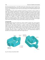
significantly BER compared to without FH at same level of SNR. From Figure 12 it can be
seen that applying FH with GFSK modulation reduces dramatically BER compared to
without FH at same level of SNR and lead to a much higher performance.
In overall, based on the evaluation results it can be concluded that applying the designed
FH schemes with certain modulations can improve their communication performances,
especially at weak SNR levels as most cases of short range wireless communications have.
6. Conclusion
As a result of the work it can be concluded that adaptive frequency hopping is a powerful
technique to deal with interference and Gilbert-Elliot channel model is a good technique to
analyze the situations of channels by categorizing the channel conditions based on their
performance as Good or Bad, and then apply adaptive frequency hopping which hops
frequencies adaptively by analyzing the state of the channel in case of environmental
problems such as interferences and noises to improve the communication performance.
Frequency hopping spread spectrum is modelled with MATLAB and three different
modulations i.e. QAM, QPSK and GFSK are studied to investigate which of these
modulations are good to apply with FHSS model. The simulation results show that applying
FHSS with QAM modulation dose not lead to a remarkable reduction of BER, but with
QPSK modulation gives a good result and reduces BER at lower SNR, while in GFSK
modulation shows a significant reduction of BER and lead to a high performance.



Fig. 10. QAM modulation
Frequency Hopping Spread Spectrum:
An Effective Way to Improve Wireless Communication Performance

201

Fig. 11. QPSK modulation


Fig. 12. GFSK modulation
Advanced Trends in Wireless Communications

202
7. References
Bates, R. J. & Gregory, D. W. (2001). Voice & Data Communications Handbook, McGraw-Hill
Osborne Media
Elliott, E. O. (1963). Estimates of error rates for codes on burst-noise channels, Bell System
Technical Journal, Vol. 42, pp. 1977-1997
Gilbert, E. N. (1960). Capacity of burst-noise channels, Bell System Technical Journal, Vol. 39,
pp. 1253-1265
Lemmon, J. J. (2002). Wireless link statistical bit error model, Institute for Telecommunication
Sciences
Liu, Y. (2008). Enhancement of short range wireless communication performance using
adaptive frequency hopping, Proceeding of 4th IEEE International Conference on
Wireless Communications, Networking and Mobile Computing, Dalian, China, Oct. 2008
Zander, J. & Malmgren, G. (1995). Adaptive frequency hopping in HF communications, IEE
Proceedings Communications, Vol. 142, pp. 99-105
Ziemer, R.; Peterson, E. R. L. & Borth, D. E, (1995). Introduction to Spread Spectrum
Communications, Prentice Hall
Part 4
Multi-Input Multi-Output Models

11
Wireless Communication: Trend and Technical
Issues for MIMO-OFDM System

Yoon Hyun Kim
1
, Bong Youl Cho
2
and Jin Young Kim
3

1,3
Kwangwoon University,
2
Nokia-Siemens Networks,
Seoul
Korea
1. Introduction
High-performance 4
th
generation (4G) broadband wireless communication system can be
enabled by the use of multiple antennas not only at transmitter but also at receiver ends. A
multiple input multiple output (MIMO) system provides multiple independent transmission
channels, thus, under certain conditions, leading to a channel capacity that increases linearly
with the number of antennas. Orthogonal frequency division multiplexing (OFDM) is
known as an effective technique for high data rate wireless mobile communication. By
combining these two promising techniques, the MIMO and OFDM techniques, we can
significantly increase data rate, which is justified by improving bit error rate (BER)
performance. In this section, we briefly describe the concept of MIMO system. Through
comparison with CDMA system, its key benefits are discussed.
1.1 Concept of MIMO system
The idea of using multiple receive and multiple transmit antennas has emerged as one of the
most significant technical breakthroughs in modern wireless communications. Theoretical
studies and initial prototyping of these MIMO systems have shown order of magnitude

spectral efficiency improvements in communications. As a result, MIMO is considered a key
technology for improving the throughput of future wireless broadband data systems
MIMO is the use of multiple antennas at both the transmitter and receiver to improve
communication performance. It is one of several forms of smart antenna technology. MIMO
technology has attracted attention in wireless communications, because it offers significant
increases in data throughput and link range without requiring additional bandwidth or
transmit power. This is achieved by higher spectral efficiency and link reliability or diversity
(reduced fading). Because of these properties, MIMO is an important part of modern
wireless communication standards such as IEEE 802.11n (Wifi), IEEE 802.16e (WiMAX),
3GPP Long Term Evolution (LTE), 3GPP HSPA+, and 4G systems to come.
Radio communication using MIMO systems enables increased spectral efficiency for a given
total transmit power by introducing additional spatial channels which can be made
available by using space-time coding. In this section, we survey the environmental factors
that affect MIMO performance. These factors include channel complexity, external
interference, and channel estimation error. The ‘multichannel’ term indicates that the
Advanced Trends in Wireless Communications

206
receiver incorporates multiple antennas by using space-time-frequency adaptive processing.
Single-input single-output (SISO) is the well-known wireless configuration, single-input
multiple-output (SIMO) uses a single transmit antenna and multiple receive antennas,
multiple-input single-output (MISO) has multiple transmit antennas and one receive
antenna. And multiuser-MIMO (MU-MIMO) refers to a configuration that comprises a base
station with multiple transmit/receive antennas interacting with multiple users, each with
one or more antennas.


Tx Rx
SISO

(a)

MIMO
Tx Rx

(b)

SIMO
Tx
Rx

(c)

MISO
Tx Rx

(d)
Fig. 1.1. Different antenna system
(a) SISO mode (b) MIMO mode (c) SIMO mode (d) MISO mode
1.2 Key benefits
1.2.1 Array gain
Array gain can be made available through processing at the transmitter and/or the receiver,
and results in an increase in average received signal-to-noise ratio (SNR) due to a coherent
Wireless Communication: Trend and Technical Issues for MIMO-OFDM System

207
combining effect. Transmit-receive array gain requires channel knowledge at the transmitter
and receiver, respectively, and depends on the number of transmit and receive antennas.
Channel knowledge at the receiver is typically available whereas channel state information
at the transmitter is in general more difficult to obtain.

Array gain means a power gain of signals that is achieved by using multiple-antennas at
transmitter and/or receiver. It is the average increase in the SNR at the receiver that arises
from the coherent combining effect of multiple antennas at the receiver or transmitter or
both. If the channel is known to the transmitter with multiple antennas, the transmitter
can apply appropriate weight to the transmission, so that there is coherent combining at
the receiver. The array gain in this case is called transmitter array gain. Alternately, if we
have only one antenna at the transmitter and no knowledge of the channel, then the
receiver can suitably weight the incoming signals so that they coherently add up at the
output, thereby enhancing the signal. This is called receiver array gain which can be
exploited in SIMO case. Essentially, multiple antenna systems require some level of
channel knowledge either at the transmitter or receiver or both to achieve this array
gain.
1.2.2 Diversity gain
In a wireless channel, signals can experience fadings. When the signal power drops
significantly, the channel is said to be in a fade and this gives rise to high BER. Diversity is a
powerful technique to mitigate fading in wireless links, so diversity is often used to combat
fading. Diversity techniques rely on transmitting the signal over multiple (ideally)
independently fading paths over time, frequency, space, or others. Spatial (or antenna)
diversity is preferred over time/frequency diversity as it does not incur expenditure in
transmission time or bandwidth.
A diversity scheme refers to a method for improving the reliability of a message signal by
using two or more communication channels with different characteristics. Diversity plays an
important role in combating fading and co-channel interference and avoiding error bursts. It
is based on the fact that individual channels experience different levels of fading and
interference. Multiple versions of the same signal may be transmitted and/or received and
combined in the receiver. Alternatively, a redundant forward error correction code may be
added and different parts of the message transmitted over different channels. Diversity
techniques may exploit the multipath propagation, resulting in a diversity gain, often
measured in decibels.
The following classes of diversity schemes can be identified

• Time diversity: Multiple versions of the same signal are transmitted at different time
instants. Alternatively, a redundant forward error correction code is added and the
message is spread in time by means of bit-interleaving before it is transmitted. Thus,
error bursts are avoided, which simplifies the error correction.
• Frequency diversity: This type of diversity provides replicas of the original signal in the
frequency domain. The signals are transmitted using several frequency channels or the
signals are spread over a wide spectrum that is affected by frequency-selective fading.
The former method can be found in coded-OFDM systems such as IEEE 802.11agn,
WiMAX, and LTE, and the latter method can be found in CDMA systems such as 3GPP
WCDMA.
• Multiuser diversity: Multiuser diversity is obtained by opportunistic user scheduling at
either the transmitter or the receiver. Opportunistic user scheduling is as follows: the
Advanced Trends in Wireless Communications

208
transmitter selects the best user among candidate receivers according to the qualities of
each channel between the transmitter and each receiver. In FDD systems, a receiver
typically feedback the channel quality information to the transmitter with the limited
level of resolution.
• Space diversity (antenna diversity): The signal is transmitted over several different
propagation paths. In the case of wired transmission, this can be achieved by
transmitting via multiple wires. In the case of wireless transmission, it can be achieved
by antenna diversity using multiple transmit antennas (transmit diversity) and/or
multiple receive antennas (receive diversity). In the latter case, a diversity combining
technique is applied before further signal processing takes place. If the antennas are far
apart, for example at different cellular base station sites or WLAN access points, this is
called macrodiversity or site diversity. If the antennas are at a distance in the order of
one wavelength, this is called microdiversity. A special case is phased antenna arrays,
which also can be used for beamforming, MIMO channels and Space–time coding
(STC). Space diversity can be further classified as follows.

- Receive diversity: Maximum ratio combining is a frequently applied diversity scheme
in receivers to improve signal quality
- Transmit diversity: In this case we introduce controlled redundancies at the transmitter,
which can be then exploited by appropriate signal processing techniques at the receiver.
There are open loop transmit diversity where transmitter does not require channel
information and closed loop transmit diversity where transmitter requires channel
information to make this possible. Closed loop transmit diversity is sometimes
regarded as a Beamforming. Space-time codes for MIMO exploit both transmit as well
as receive diversity schemes, yielding a high quality of reception.
- Polarization diversity: Multiple versions of a signal are transmitted and/or received via
antennas with different polarization. A diversity combining technique is applied on the
receiver side.
- Cooperative diversity: Achieves antenna diversity gain by using the cooperation of
distributed antennas belonging to each node.
1.2.3 Multiplexing gain
Spatial multiplexing gain is achieved when a system is transmitting different streams of data
from the same radio resource in separate spatial dimensions. Data is hence sent and received
over multiple channels - linked to different pilot signals, over multiple antennas. This results
in capacity gain at no additional power or bandwidth.
Spatial multiplexing is transmission techniques in MIMO wireless communication to
transmit multiple data signals from each of the multiple transmit antennas. Therefore, the
space dimension is reused, or multiplexed, more than one time.
If the transmitter is equipped with N
T
antennas and the receiver has N
R
antennas, the
maximum spatial multiplexing order is

min( , ).

sTR
NNN
=
(1-1)
If a linear receiver is used, this means that
s
N streams can be transmitted in parallel, ideally
leading to an
s
N increase of the spectral efficiency. The practical multiplexing gain can be
limited by spatial correlation and the rank property of the channel, which means that some
of the parallel streams may have very weak or no channel gains.
Wireless Communication: Trend and Technical Issues for MIMO-OFDM System

209
1.2.4 Interference reduction
Fig. 1.2 presents a K-user MIMO interference channel with K transmitter and receiver pairs.
The k-th transmitter and its corresponding receiver are equipped with
k
M
and
k
N antennas
respectively. The k-th transmitter generates interference at all lk
≠
receivers. Assuming the
communication channel to be frequency-flat, the
1
k
N

C
×
received signal
k
y
at the k-th
receiver, can be represented as

1
,
K
kkkk kllk
l
lk
y
Hx Hx n
=
≠
=+ +
∑
(1-2)
where
kl
NM
kl
HC
×
∈ represents the channel matrix between the -thl transmitter and k-th
receiver,
k

x is the
1
k
M
C
×
transmit signal vector of the k-th transmitter and the
1
k
N
C
×
vector
k
n represents AWGN with zero mean and covariance matrix
kk
nn
R . Each entry of the
channel matrix is a complex random variable drawn form a continuous distribution. It is
assumed that each transmitter has complete knowledge of all channel matrices
corresponding to its direct link and all the other cross-links in addition to the transmitter
power constraints and the receiver noise covariances.
We denote by
k
G , the
kk
M
d
C
×

precoding matrix of the k-th transmitter. Thus
kkk
xGs= ,
where
k
s is a 1
k
d
×
vector representing the
k
d independent symbol streams for the k-th
user pair. We assume
k
s to have a spatiotemporally white Gaussian distribution with zero


Fig. 1.2. MIMO Interference Channel
Advanced Trends in Wireless Communications

210
mean and unit variance,
~(0, )
kdk
sI
Ν
. The k-th receiver applies
kk
dN
k

FC
×
∈
to suppress
interference and retrieve its
k
d desired streams. The output of such a receive filter is then
given by

1
K
kkkkkk kklllkk
l
lk
rFHGs FHGsFn
=
≠
=+ +
∑
(1-3)
Note that
k
F does not represent the whole receiver but only the reduction from a
k
N -
dimensional received signal
k
y
to a
k

d -dimensional
k
r , to which further receive processing
is applied.
Co-channel interference arises due to frequency reuse in MIMO wireless channels. When
multiple antennas are used, the differentiation between the spatial signatures of the desired
signal and co-channel signals can be exploited to reduce interference. Interference reduction
requires knowledge of the desired signal’s channel. Exact knowledge of the interferer’s
channel may not be necessary. Interference reduction can also be implemented at the
transmitter, where the goal is to minimize the interference energy sent toward the co-
channel users while delivering the signal to the desired user. Interference reduction allows
aggressive frequency reuse and thereby increases multicell capacity. We note that in general
it is not possible to exploit all the leverages of MIMO technology simultaneously due to
conflicting demands on the spatial degrees of or number of antennas. The degree to which
these conflicts are resolved depends upon the signalling scheme and transceiver design.
2. MIMO system
In this section, the MIMO channel model is discussed first, which are deterministic, and
frequency flat or selective fading channels. This study will be carried out mathematical
derivation of the capacity in each MIMO channel. We begin with basic system capacities
which compare SISO, SIMO and MIMO, and then we explore to general case that the system
has
M
T
transmit antennas and N
R
receive antennas. Finally, fundamental capacity limits for
transmission over MIMO channels is discussed
Many kinds of signal encoding schemes that support multiple antenna systems have well
been studied [2]. Among them, the primary ones include Bell Labs Layered Space Time
(BLAST), space-time trellis codes (STTC), space-time block codes (STBC) and cyclic delay

diversity (CDD) and so on. So, the latter part in this chapter, we introduce STBC and STTC
signal models for transmitter /receiver structure in MIMO system.
2.1 MIMO channel model
We consider MIMO channels with
N
T
transmit and N
R
receive antennas. The block diagram
of such a MIMO channel model is shown in Figure 2.1.
The channel matrix H is a N
R
× N
T
complex matrix with

1,1 1,2 1,
2,1 2,2 2,
,1 ,2 ,
.
T
T
RR RT
N
N
NN NN
hh h
hh h
hh h
⎡

⎤
⎢
⎥
⎢
⎥
=
⎢
⎥
⎢
⎥
⎢
⎥
⎣
⎦
H




(2-1)
Wireless Communication: Trend and Technical Issues for MIMO-OFDM System

211
The component of the matrix H,
,i
j
h is the coefficient of the each channel from the jth
transmit antenna to the
ith receive antenna. We suppose that the power of the received
signal for each receive antennas is equal to the sum of transmit power

E
s.
Consequently, we
acquire the normalization value of the channel matrix H, for a deterministic channel
condition as follow,

2
,
1
, 1, 2, , .
T
N
i
j
TR
j
hNi N
=
==
∑
… (2-2)
If the channel coefficients are random, the normalization value will apply to the expected
value. The received signal at
ith receive antenna is given by

,
1
() () () (), 1,2,
T
N

i
jj
iR
j
y
thtstnt i N
=
=⋅+ =
∑
… , (2-3)
where,
s
j
(t) is the transmit signal at jth transmit antenna and n
i
(t) is additive white Gaussian
noise (AWGN) in the receiver with zero mean and
2
σ
variance. In above equation, a
transmit signal
s
j
(t) from each transmit antenna is added to the signal of each receive
antenna.
2.1.1 Deterministic channel
To introduce the characteristics of the random channel matrix H, first we need to study the
deterministic channel model. Coefficient of the deterministic channel model H is fixed on H. In
other words, the deterministic channel coefficient H is known at the transmitter and receiver.
2.1.2 Flat fading channel

Suppose that the delay spread (
τ
max
) in the MIMO channel is much smaller than the signal
bandwidth (
BW), i.e.,
τ
max
<< 1/BW, the channel is said to be frequency flat fading channel.
Frequency flat fading channel has the properties that are known to be exact in non line-of-
sight (NLOS) environment with rich scattering and sufficient antenna spacing between
transmitter and receiver antennas.
2.1.3 Frequency selective fading channel
Similarly, if the signal bandwidth and MIMO channel delay spread product satisfies
τ
max
>>
0.1/BW, the MIMO channel is said to be frequency selective. The transfer function of the
frequency selective MIMO channel is as follow,

0
() ()exp( 2 )
f
jfd
τ
πτ τ
∞
=−
∫
HH . (2-4)

2.2 Capacity of each MIMO channel
In this subsection, the capacity of the MIMO channels is introduced. The capacity is defined
as the maximum possible transmission rate when the probability of error is almost zero. The
capacity of MIMO channel is defined,

()
max ( ; )
fs
CI
=
sy , (2-5)
Advanced Trends in Wireless Communications

212
where,
f(s) is the probability distribution function (PDF) of the transmit signal vector s and
I(s;y) is the mutual information between transmit signal vectors s and receive signal vector
y. The mutual information is given by

(; ) ( ) (|)IHH
=
−sy y y s , (2-6)
where,
H(y) is the entropy of the receive signal vector y, and H(y|s) is the conditional
entropy of the receive signal vector y. The conditional entropy
H(y|s) is identical to H(n)
because the transmit signal vector s and noise vector n are independent. So, equation (2-6) is
written as

(; ) ( ) ( )IHH=−sy y n . (2-7)

For maximize the mutual information,
I(s;y), reduces to maximizing H(y). Consequently,
mutual information
I(s;y) in equation (2-7) is given by,

2
0
(; ) logdet( ) /
R
S
H
N
T
E
IbpsHz
NN
=+
SS
sy I HR H , (2-8)
where,
R
N
I is an N
R
× N
R
identity matrix, E
S
is the power across the transmitter irrespective
of the number of antennas

N
T
, R
SS
is the covariance matrix for transmit signal and the
superscript
H
stands for conjugate transposition. From equation (2-8), the general capacity of
the MIMO channel is

2
,( )
0
max log det( ) /
R
T
S
H
N
tr N
T
E
CbpsHz
NN
=
=+
SS SS
SS
RR
IHRH. (2-9)

2.2.1 Capacity of a deterministic MIMO channel
As we mentioned previous, the deterministic channel coefficient H is known at the
transmitter and receiver. However, to acquire channel coefficient at the transmitter is very
difficult in practical MIMO systems. In the case that the MIMO system do not knows the
channel coefficient at the transmitter, generally called an open-loop system, it is a good
assumption that the transmitted signals from each transmit antenna has equal power. This
condition results in the covariance matrix is identical to the identity matrix,
T
N
I=
SS
R . So,
from equation (2-8), equal powered mutual information is given by,

2
0
(; ) logdet( ) /
R
S
H
eq N
T
E
IbpsHz
NN
=+sy I HH
, (2-10)
where the subscript “eq” stands for “equal power”.
Mutual information in equation (2-10) can be calculated by positive eigenvalues of the
channel matrix

H
HH . If r is the rank of the matrix H and ,1,2,
i
ir
λ
=
… are the non-zero
eigenvalues of the matrix
H
HH , the mutual information in equation (2-10) is re-written
as

2
0
1
(; ) log(1 ) /
r
S
eq i
T
i
E
IbpsHz
NN
λ
=
=+
∑
sy . (2-11)
Wireless Communication: Trend and Technical Issues for MIMO-OFDM System

213
2.2.2 Capacity of frequency selective fading MIMO channel
In this subsection, we discuss the capacity of MIMO channel in frequency selective fading
condition. The capacity of frequency selective fading channel can be obtained by dividing
the whole bandwidth into
N sub-channel. This results in each sub-channel having BW/N
bandwidth. If
N is not sufficient large, each sub-channel is undergone frequency selective
fading. So, we can derive the capacity of
ith sub-channel of frequency selective fading
channel is given by

,
,2
0
(; ) logdet( ) /
R
Si
H
ifs N i i
T
E
IbpsHz
NN
=+sy I HH
, (2-12)
where, subscript ‘
fs’ stands for ‘frequency selective’, E
S,i

is the energy allocated to the ith
sub-channel and
H
i
is the N
R
× N
T
sub-channel matrix.
And the ergodic capacity of the frequency selective fading MIMO channel is given by [
H.
Jafarkhani
(p.38)] as follow,

,
(; )
f
si
f
s
CI
ε
=
⎡
⎤
⎣
⎦
sy
. (2-13)
2.3 Transmit signal structure for space time block coding

In this subsection, the basics of the Alamouti STBC with two antennas at the transmitter is
briefly introduced. A block diagram of the Alamouti’s space time block encoder is shown in
Fig. 2.1. The information sources are modulated with an M-ary modulation scheme. Then,
the encoder takes a group of two modulated symbols. The each group consist of the two
modulated symbol s
1
and s
2
in each encoding operation and then it sends to the transmit
antennas according to the block code matrix,

*
12
*
21
ss
S
ss
⎡
⎤
−
=
⎢
⎥
⎢
⎥
⎣
⎦
. (2-14)
In above equation (2-14), the first column stands for the first transmission symbol period

and the second column stands for the second transmission symbol period. Similarly, the first
row corresponds to the symbols which are transmitted from the first antenna and the second
row corresponds to the symbols which are transmitted from the second antenna. In detail,
the first antenna transmits s
1
and the second antenna transmits s
2
during the first symbol
period at the same time. Similarly, for the second period, first antenna transmits –s
2
* and
simultaneously, second antenna transmits s
1
*. Note that superscript ‘*’ stands for the
complex conjugate of the symbol. By using the Alamouti’s space time coding, we can
transmit symbol both in space and time. This is “space time block coding”.
Symbol groups of the each transmit antenna are given are

*
11 2
*
22,1
[, ]
[ ]
ss
ss
=−
=
S
S

, (2-15)
where, S
1
is the first symbol group from the first antenna and S
2
is the second symbol group
from the second antenna.
In equation (2-15), two group symbols are orthogonal each other. Here, orthogonal means
Advanced Trends in Wireless Communications

214

Input
Information
Modulation
STBC
Encoder
Tx1
Tx2

Fig. 2.1. A block diagram of the STBC system
that the inner product of S
1
and S
2
is zero. This orthogonal relationship is given by,

**
12 12 21
0ss ss

⋅
=−=SS
. (2-16)
2.4 Receiver structure for space time block coding
If we suppose that the system has one antenna at receiver and two antennas at transmit
antenna, the receiver structure is illustrated as Fig. 2.2.
The channel coefficient from transmit antenna 1 and 2 are defined as
h
1
(t) and h
2
(t). As these
channel coefficients are generally constant across two consecutive symbol periods,
h
1
(t) and
h
2
(t) are given by,

1
2
11 1
22 2
() ( )
() ( ) ,
j
j
ht ht T he
ht ht T he

θ
θ
=+=
=+=
(2-17)
where
i
h and
i
θ
are the amplitude gain and phase shift for the path from each transmit
antenna to the receive antenna.
At the receiver, the received signals can be expressed as,

111221
**
2 12212
,
rhshsn
rhshsn
=++
=− + +
(2-18)

where, n
1
and n
2
are independent complex variables with zero mean and unit variance,
representing additive white Gaussian noise (AWGN) samples.

If the channel coefficients h
1
and h
2
can be recovered perfectly at the receiver, the received
signal can be combined as follows,

**22* *
11122 1 211122
** * 2 2 * *
22112 1 221221
()
() ,
shrhr shnhn
shrhr shnhn
αα
αα
=+ =+ + +
=−=+ −+


(2-19)
and these estimated signals are sent to the maximum likelihood detector, which minimizes
the following decision metric

2
*
12
*
212

2
22111
shshrshshr −++−− . (2-20)
Wireless Communication: Trend and Technical Issues for MIMO-OFDM System

215

Fig. 2.2. Receiver structure for space time block coding
To expand and delete terms that are orthogonal of the code words, the equation (2-20) is
reduced by [H. Jafarkhani (p.57)] to,

2
1
2
2
2
1
2
12
*
2
*
11
)1( sshrhr −++−+
αα
, (2-21)
And,

.)1(
2

2
2
2
2
1
2
21
*
2
*
21
sshrhr −++−−
αα
(2-22)
Finally, for PSK signal, maximum likelihood detector calculate signal as follow,

kissdssd
kjij
≠∀≤ ),
ˆ
(),
ˆ
(
22
, (2-23)
where,
2
**2
))((),( yxyxyxyxd −=−−=
.

3. Technology challenges and issues for MIMO-OFDM system
3.1 Data throughput
3.1.1 Adaptive modulation and coding
Adaptive modulation and coding (AMC) is a technical term used in wireless
communications to achieve maximum data throughput. AMC denotes the matching of
Advanced Trends in Wireless Communications

216
coding, modulation and other parameters to the conditions on the channel, as the path loss,
the interference, the sensitivity of the receiver and available transmitter power margin.
The MIMO-OFDM system typically consists of convolutional encoder, modulation, inverse
fast Fourier transform (IFFT), injection of guard interval (GI) and pre-coder. And the multi-
user MIMO OFDM system with AMC is depicted in Fig. 3.1.


Fig. 3.1. Multi-user MIMO OFDM with AMC
Wireless Communication: Trend and Technical Issues for MIMO-OFDM System

217
The pre-coded signals are summed at each antenna of a base station. The pre-coding matrix
is computed by using channel matrix which is estimated from the feedback from each user
and base station.
As an example, the scheme here uses AMC that has 6 modulation and coding scheme (MCS)
levels. The coding rate of convolutional encoder and the modulation order are changed per
MCS level. MCS level is usually decided by SNR which is estimated and computed at the
channel estimator of each user.
In Table 3.1, the coding rate and the modulation order are tabled according to SNR in the
multi-user and the single-user system. The AMC of the scheme uses BPSK, QPSK, 16QAM
modulation and 2/3, 1/2 coding rate at convolution encoder. The SNR range is defined as
the SNR range that the error performance of each user is 10

-4
.

AMC
Modulation Coding rate
SNR[dB] of
Single-user
(IEEE 802.11n)
SNR[dB] of
Multi-user
(IEEE 802.11n)
1/2 0<SNR≤2.5 0<SNR≤2.5
BPSK
3/4 2.5<SNR≤4 2.5<SNR≤4
1/2 4<SNR≤6.5 4<SNR≤7
QPSK
3/4 6.5<SNR≤19.5 7<SNR≤19.5
1/2 19.5<SNR≤37 19.5<SNR≤38
16QAM
3/4 37<SNR 38<SNR
Table 3.1. AMC selection according to SNR
The process at the user’s side is processed in reverse order of the side of the base station.
3.1.2 CP reduction algorithm
In wireless mobile communication systems, there are Doppler shift and delay spread that
introduce significant problem to system performance. Doppler shift introduce the channel
fading effect with frequency translation caused by movement of mobile station. Doppler
shift will be positive or negative depending on whether the mobile receiver is moving
toward or away from the base station. Delay spreads are resulted in multiple versions of the
transmitted signals that arrive at the receiving antenna, it causes to displace with respect to
one another in time and spatial orientation. The random phase and amplitudes of the

different multipath components cause fluctuation in signal strength, thereby inducing small-
scale fading, signal distortion, or both. Multipath propagation often lengthens the time
required for the baseband portion of the signal to reach the receiver, which can cause signal
smearing, which is known as inter-symbol interference (ISI).
To prevent ISI effects, first, OFDM divides the high rate data stream into a number of
parallel sub-streams. Next, they are modulated onto different orthogonal sub-carriers, thus
it has lower symbol rate, and then a cyclic prefix (CP) is added to the head of each symbol to
try to eliminate the effect ofISI.
Although CP insertion highly improves the performance of OFDM systems, fixed CP length
introduces overhead to overall system. For example, in 802.11a wireless local area network
(WLAN) system where CP length is fixed by proportion 1/5 of data block size, the time and
energy for CP are wasted.
To reduce the time and energy wasted, adaptive CPs length using correlation value of
receive signals can be used. First, we do not consider the received signals whose power level
Advanced Trends in Wireless Communications

218
of received signal is lower than noise level, and then, search for correlation value between
the first arrived signal and the last delayed signal. Finally, CP lengths are controlled by
correlation value from the feedback information of receiver. To control the CP length, we
assume that channel varies very slowly. So next symbol length applying adaptive CP
control is added to some bit for minimization ISI. However, if every symbol’s CP length is
changed, next symbol’s CP length is very short. For this reason, in deep fading channel
condition, BER is increased.
Fig. 3.2 shows the OFDM system with adaptive CP length. Data block is fed to serial-to-
parallel (S/P) block and is modulated by sub-carriers. The modulated data block is passed
by IFFT as follow equation.

1
0

12
exp , 0 ,
N
ni
i
ik
xX iN
N
N
π
−
=
⎧⎫
=≤≤
⎨⎬
⎩⎭
∑
(3-1)
Where, N represents the number of FFT points. CP, which is a proportion of data block
size, is added to ahead of the data as shown in equation (3-2).

.1,,1,0,, ,)( −−== NGnnxx
N
g
n

(3-2)
where G represents length of CP. So, equation (3-3) represents signals with CP inserted. The
signals that passed by channel can be represented as follow equation.

),()()()( tnthtxtr
n
g
nn
+∗=
(3-3)
where, ‘∗’, n(t) and
)(th
n
are represent convolution sum, AWGN, and impulse response of
the Rayleigh fading channel, respectively. Rayleigh fading channel has PDF as follow.

2
22
exp 0 .
()
2
0 0
rr
r
pr
r
σσ
⎧
⎛⎞
−
≤
≤∞
⎪
⎜⎟

=
⎨
⎝⎠
⎪
<
⎩
(3-4)
where,
2
σ
is the time-average power of the received signal.
Transmitted signals are received with reflection, refraction and diffraction. First, we do not
consider the received signals whose power level of received signal is lower than noise level,
and then, search for correlation value between the first arrived signal and the last delayed
signal. Finally, CP lengths are controlled by correlation value from the feedback information
of receiver in CP controller of Fig. 3.3.
As shown above Figures, CP length is controlled by correlation value and transmited /
received signal are re-calculated as follow.

(), , 0, , 1,
g
nN
xxnnG N
=
=− −



(3-5)

() () () ().
g
nnn
rt x t ht nt=∗+

(3-6)
We obtain the simulation results about data rate and power loss as to mobile speed. Fig. 3.4
shows the gain of data rate when mobile speed is 20km/h. Red line is the conventional OFDM
system with fixed CPs length and blue line is the OFDM system with adaptive CPs length.
Wireless Communication: Trend and Technical Issues for MIMO-OFDM System

219

Fig. 3.2. OFDM system with adaptive CP length
In the case of using fixed CPs, there is no gain of data rate. However, the OFDM system
using adaptive CP length is able to obtain the gain in data rate about 10Mbps with
transmission of 1000 frames.
3.2 Antenna issues
Antenna element numbers and inter-element spacing are key parameters in MIMO system,
and especially the latter is really important for the high spectral efficiencies of MIMO to be
realized.
Advanced Trends in Wireless Communications

220
Base stations with large numbers of antennas pose environmental concerns. Hence, the
antenna element numbers are limited to a modest number, with an inter-element spacing of
around 10
λ.
The large spacing is because base stations are usually mounted on elevated positions where
the presence of local scatterers to decorrelate the fading cannot be always guaranteed. As an

example in four antenna system, four antennas can fit into a linear space of 1.5 m at 10
λ
spacing at 2 GHz using dual polarized antennas. For the terminal, (1/2)
λ spacing is usually


Fig. 3.3. Correlation value of received signals (20km/h)


Fig. 3.4. Data rate of proposed scheme (20km/h)
Wireless Communication: Trend and Technical Issues for MIMO-OFDM System

221
sufficient to ensure a fair amount of uncorrelated fading because the terminal is present
amongst local scatterers and quite often there is no direct path. The maximum number of
antennas on the terminal is envisaged to be four (or more), though a lower number, say two,
is an implementation option. Four dual polarized patch antennas can fit in a linear space of
7.5 cm. These antennas can easily be embedded in casings of lap tops. However, for
handsets, even the fitting of two elements may be problematic. This is because, the present
trend in handset design is to imbed the antennas inside the case to improve look and appeal.
This makes spacing requirements even more critical.
3.3 Precoding schemes for multi-user MIMO system
Precoding scheme linearizes each layer of MIMO and makes beamforming possible. Default
precoder can be unitary precoder based on Fourier matrix, and system can utilize specific
precoder based on precoder codebook transimitted from mobile station. There are two types
of precoder codebook, knockdown precoder and readymade precoder.

Demultiplexer
AMC
AMC

Precoder
OFDM
Modulator
OFDM
Modulator
Receiver
Precoding
Rank
CSI
CSI

Fig. 3.5. MIMO-OFDM system with a precoder
Knockdown precoder uses the predefined matrix of prime numbers for the formulation of
precoder. Then mobile device returns the information about suitable index and column of
matrix. And the base station uses the information to select a precoder. This is typically
referred to as codebook-based beamforming.
Readymade precoder utilizes the
M predefined matrices for the precoder. The mobile device
feeds the information about the index of the proper matrix back to the base station. Then the
base station makes a use of the matrix.
3.4 System complexity
The implementation complexity of the MIMO system represents a substantial increase over
existing devices. There are two primary areas of increased complexity associated with the
MIMO system: RF and baseband processing. An assessment of FPGA implementation
shows that a 2×2 implementation is roughly three times the baseband complexity of current
devices. A 4×4 implementation is about eight times the baseband complexity of current
devices. Given the continuous increase in transistor density, we anticipate that the baseband
processing is not a significant cost driver for next-generation technology.
Advanced Trends in Wireless Communications

222
While additional RF receive and transmit chains are required to support MIMO, some parts
of the chains, such as the local oscillator and clock generation circuitry, can be shared. In
addition, the transmit power requirement per power amplifier decreases directly in
proportion to the number of antennas employed.
Improved support for sleep and idle modes in the MAC will permit highly efficient power
utilization for battery-powered devices, achieving charge cycles equivalent to or better than
those cell phones achieve today.
4. Acknowledgement
This work was, in part, supported by Basic Science Research Program through the National
Research Foundation of Korea(NRF) funded by the Ministry of Education, Science and
Technology(MEST)"(No. 2010-0022629) and, in part, supported by Kwangwoon university.
5. References
A. Goldsmith; S. A. Jafar; N. Jindal, & S. Vishwanath, (2003). Capacity limits of MIMO
channels,
IEEE J. Select. Areas Commun., vol. 21, no. 5, pp. 684-702.
C. Windpassinger; R. F. H. Fischer; T. Vencel & J. B. Huber, (2004). Precoding in multi-
antenna and multi-user communications,
IEEE Trans. Wireless Commun., vol. 3, no.
4, pp. 1305-1316.
D. Tse & P. Viswanath, (2005).
Fundamentals of Wireless Communication, 0521845270,
Cambridge University Press.
G. Bauch & J. Shamim Malik, (2004). Parameter optimization, interleaving and multiple
access in OFDM with cyclic delay diversity,
IEEE Trans. Veh. Technol., vol. 1, pp. 505
– 509.
H. Jafarkhani, (2005).
Space-Time Coding - Theory and Practice, 100521842913, Cambridge
University Press.

J. G. Proakis, (2001).
Digital Communications (4th ed.), 0072321113, McGraw-Hill, New York.
J. Y. Kim, (2008).
MIMO-OFDM System for High-Speed Wireless Communication Component,
9788956674599, Gybo Publisher, Seoul, Korea.
L. Hanzo; M. Munster; B. J. Choi, & T. Keller, (2003).
OFDM and MC-CDMA for Broadband
Multi-User Communications, WLANs and Broadcasting
, 0470858796, John Wiley &
Sons.
M. Jankiraman
, (2004). Space-Time Codes and MIMO Systems, 1580538657, Artech House
Publishers.
Q. H. Spencer; C. B. Peel; A. L. Swindlehurst & M. Haardt, (2004). An introduction to the
multi-user MIMO downlink,
IEEE Commun. Mag., vol. 42, no. 10, pp. 60-67.
Q.H. Spencer, et al., (2000). Modeling the statistical time and angle of arrival characteristics
of an indoor environment,
IEEE J. Select. Areas Commun., vol. 18, no. 3, pp. 347-360.
Siavash M Alamouti, (1998). A simple transmit diversity technique for wireless
communications,
IEEE J. Select. Areas Commun., vol. 16, no. 8, pp. 1451-1458.
Ijaz Naqvi
1
and Ghaïs El Zein
2
1
LUMS School of Science and Engineering (SSE) Sector U, D.H.A. Lahore Cantt
2
European University of Brittany (UEB)

INSA, IETR, UMR 6164, F-35708, 20 avenue des Buttes de Coesmes, 35708 Rennes
1
Pakistan
2
France
1. Introduction
Ultra wide band (UWB) technology gained a renewed interest after February 2002, when
the Federal Communications Commission (FCC) approved the First Report and Order
(R&O) for commercial use of UWB technology under strict power emission limits for
various devices. The permission to transmit signals in a wide unlicensed band, opened
the doors for the coexistence of UWB technology along with other narrow band and
spread spectrum technologies. In UWB communication, extremely narrow RF pulses are
employed to communicate between transmitters and receivers. Because of its extremely wide
bandwidth, UWB signals result in a large number of resolvable multi-paths and thus reduce
the interference caused by the super position of unresolved multi-paths. However, it also
results in a complex receiver system. To collect the received signal energy, several kinds of
receivers can be applied such as transmit-reference, Rake or decision feedback autocorrelation
receiver. The later two techniques are quite complex while the former decreases the data rate
of the system. One way to overcome these drawbacks is to make use of a technique that shifts
the design complexity from the receiver to the transmitter.
Time Reversal (TR) has been proposed as a technique to shift the design complexity from the
receiver to the transmitter. Classically, TR has been applied to acoustics Fink (1992); Fink &
et. al. (2000) and underwater systems Edelmann et al. (2002), but recently, it has been widely
studied for broadband and UWB communication systems Khaleghi et al. (2007)- Oestges et al.
(2004). The received signal in a TR system is considerably focused in spatial and temporal
domains and can be received using simple energy threshold detectors. The temporal and
spatial focusing of the TR scheme improves with the bandwidth of the signal, therefore,
systems with ultra wide bandwidth are inherently suitable for the TR scheme. One of the
very first experimental study for TR with wideband electromagnetic waves is carried out in
Lerosey et al. (2006). In a TR UWB communication systems, a time-reversed channel impulse

response (CIR) is employed as a transmitter pre-filter. The TR technique comprises of two
steps. In the first step, the CIR is estimated at the transmitter end. In the second step, the
complex conjugated and time-reversed CIR is transmitted in the same channel. The TR wave
then propagates in an invariant channel following the same paths in the reverse order. Finally
Time Reversal Technique for Ultra Wide-band
and MIMO Communication Systems
12