Advanced Trends in Wireless Communications Part 9 ppt
Bạn đang xem bản rút gọn của tài liệu. Xem và tải ngay bản đầy đủ của tài liệu tại đây (1.12 MB, 35 trang )
Advanced Trends in Wireless Communications
270
environment (Tadakamadla, 2006). These objects induce a signal reflections problem and in
a RSSI measurement this reflected signal can add to the received and measured signal
without system knowledge.
If target node is in the middle of two metallic objects this could be a serious problem,
because target node can communicate but signal reflections make target node estimate other
position than the correct position. To improve a good distribution some distance from nodes
to this metallic objects are sufficient to decrease the signal reflection errors.
The weather conditions, like temperature, relative humidity and pressure, in indoors
environment, could influence the final result in the localization system. Equation (1a) shows
that the RSSI measurement has a relationship with the RF propagation parameters A (dBm)
and n
Ai
(i = 1,…,n). These parameters change with these weather conditions and have
different values as the signal attenuation in the atmosphere is not the same for all
conditions. So, if RF propagation parameters are different, RSSI measurement changes for
the same position. To prevent this error, target node has to know the accurate RF
propagation parameters. The implemented framework, in this study, has a function that
estimates the signal propagation parameters without the measurement of temperature,
relative humidity and pressure. This function implements a mathematical process to
estimate the RF propagation parameters but this process also depends on the RSSI
measurements. So the measurement of temperature, relative humidity and pressure with
this process could help to find better accurate RF propagation parameters. In addition,
weather conditions also influence electronic components such as integrated circuits and
batteries. Experimental results show, meanwhile, that if temperature and humidity do not
change more than 10 % then RSSI measurements are not changed by these conditions. In
fact, in indoors industrial environments, temperature and humidity usually do not change
significantly in one day. This is confirmed by experimentation as humidity does not change
in the same location and temperature also remains constant in one day in the same location.
Because in indoors industrial environments, temperature and humidity are nearly constant
in one day, RF propagation parameters A (dBm) and n
Ai
(i = 1,…,n) need only to be adapted
periodically (i.e. to perform system calibration). On the other hand, calibration can be made
in an automatic way by the localization framework.
3.1.2 Random errors
Random errors are also possible to compensate, but a better result is not guaranteed (Peneda
et al., 2009). Signal reflection causes a random error because it is impossible to detect if a RF
signal is reflected or not. Decreasing the signal reflection effect is possible as suggested
previously. In addiction, signal diffraction and scattering are also found as random errors
(Tadakamadla, 2006).
Transmission power and transmission frequency could induce some errors to the system. If
power transmission is not controlled, all localization system fails because, to the same
distance and the same RF propagation parameters, RSSI measurement becomes different.
Also, due to electronics tolerance, some frequency deviations may appear which introduce
errors.
RSSI measurement may not have enough resolution because it does not make a strong
contribution to localization error. RSSI measurement of 1 dBm resolution is sufficient to not
introduce conversion errors, because these errors do not have an influence to the localization
accuracy. Other errors such as multi-path and interferences are the dominant contributions
to localization errors.
Indoors Localization Using Mobile Communications Radio Signal Strength
271
3.2 Fixed nodes distribution
In this sub-section, fixed nodes distribution considerations are described, because this
subject is very important to have good system performance. The distribution of fixed nodes
is very important for the trilateration algorithm to be successful. Distribution of fixed nodes
is dependent on the building lay-out (e.g. product buffers, machines, people walking paths)
and building dimensions. In this line of thought, the fixed nodes distribution has to be a
compromise between number of nodes and localization of them. Using trilateration method,
at least three fixed nodes should be in range of a mobile node for trilateration to be possible
to be performed. In practice, due to limitations in battery of fixes nodes or to obstacles in the
middle of communicating nodes, at least four fixed nodes are adopted for this purpose. Four
nodes at the worst case are adopted in order to face system difficulties such as node low
battery voltage (i.e. needing to be replaced) or obstacles in range of the communication link
which deteriorates RSSI measurement.
Also, at locations where product buffers are located, fixed node concentration is intended to
be higher. Product buffers which have dimensions dependent on the requirements of
storage space are also evaluated in terms of node concentration. Node distribution has to be
rationalized in terms of cost with factors such as of battery replacement, software updates of
reconfigurations, nodes replacement, etc. On the other hand, a zone that is better to make
calibration of RF propagation parameters can be identified to be adopted by this system.
There is a need of identifying several calibration zones and if a product buffer is very large
then several calibration zones inside it can be chosen. Each calibration zone is chosen in
order to identify typical RF propagation parameters A (dBm) and n
Ai
(i = 1,…,n). This
procedure is applied in warehouses where this system is deployed.
This system is intended to be a modular system in terms of easy setup and of specific
applications independence. As much more nodes localization system has the final result
accuracy is better. Also, distribution can not have an exceeding number of nodes, because
this fact increases costs. Maintenance of system nodes also increases cost, so the higher the
number of nodes the higher the system cost. Nodes distribution can be adapted to lay-out of
environment in order to take advantage of more important zones where more mobile nodes
are located (accuracy can be improved with more placed beacons). Distribution also has to
take into consideration the metallic objects placed in industrial environment. Because of
these limitations, the modularity of the systems becomes reduced and so these are some
limitations of the localization system. As a communications framework can be adopted by
this localization system, it may be necessary to add more fixed nodes to existing network in
order to make possible locating mobile nodes. This is a constraint to the modular and low-
cost localization system properties.
4. Error mitigation and experimental results
RSSI measurement accuracy is critical to get acknowledge on position in a localization
system. A bad RSSI acquisition value makes localization system to have poor estimation.
This makes the entire system to fail and there is no way to detect it. In order to improve
localization system results, some compensation filters are applied in RSSI measurement
process. Power consumption in ZigBee networks is low. Nevertheless, for reducing power
consumption, the nodes should only communicate when necessary, transmitting power
should be low but significant and therefore the system is able to perform well without the
need of replacing batteries too many times.
Advanced Trends in Wireless Communications
272
This section presents some experimental results on RSSI measurements and on different
height of beacons and of mobile node considerations which have to be taken into account.
4.1 Filters
Some measurement filters can be adopted to improve RSSI acquisition quality, namely that
in equation (2) and others which save and compare past RSSI acquisitions and outputs most
repeated RSSI value.
(
)
(
)
(
)
ii i
acquired measured acquired
kk kinRSSI 0.75 RSSI 0.25 RSSI 1 , 1, ,=⋅ +⋅ − = (2)
In equation (2), variable RSSI
acquired
is post-processed RSSI value and RSSI
measured
is RSSI value
in raw input just after measurement. Parameter k is acquisition value order index.
Measure N RSSI samples
w
1
/N > 0.7 ?
(w
1
+ w
2
)/N > 0.8 ?
m = 1
m = 2
yes
yes
no
no
(w
1
+ w
2
+ w
3
)/N > 0.9 ?
m = 3
Ignore
this set
yes
no
Fig. 2. Weighted-mean filter (3) algorithm
Weighted-mean filter (3) provides an average of the most repeated RSSI in set values. In set
values there are some different RSSI values but only the most repeated values (one, two or
Indoors Localization Using Mobile Communications Radio Signal Strength
273
three different values) are considered. If there are more than three most repeated different
values, the set values have too much variations and it is better not to work with this set.
wwmwm
m
ww w
m
ww w
1122
12
RSSI RSSI RSSI
RSSI 3
+++
=
≤
+++
(3)
In equation (3) w
i
(i = 1,…,m) is the number of repetitions of a RSSI value, and RSSI
wi
(i = 1,…,m) is RSSI sample value repeated with number of repetitions w
i
(i = 1,…,m). Figure 2
depicts filter (3) algorithm.
From knowledge of signal propagation conditions it is reasonable to estimate a signal level
threshold which allows distinguishing ‘good’ measurements from ‘bad’ measurements. So,
if w
1
is larger than 70 % of the measurements then RSSI = RSSI
w1
is considered, else if w
1
+ w
2
is larger than 80 % of them then m = 2 is considered.
These two types of filters have some differences between them. The first filter (2) is applied
for every RSSI measurement in the sample. So it is difficult to get which RSSI measurement
is good. The set of measurements in a sample, from which measurements are more constant,
is considered as the good RSSI value. The second filter (3) is applied only after the sample
set of RSSI measurements is completed and it ignores the measurements that have a low
repeatability, which are considered as errors.
Filter (3) assumes that if w
1
is larger than 70 % of the measurements then RSSI = RSSI
w1
is
considered. RSSI is measured with a resolution of 1 dBm. So, for example, if w
1
is 70 % and
w
2
is 30 % and RSSI
w1
= —40 dBm and RSSI
w2
= —39 dBm, then filter (3) outputs
RSSI = —40 dBm. This fact is supported by the reason that having another scheme of
calculating RSSI with for example an arithmetic mean leads to an output that is not
appropriate for dealing with practical RSSI measurement accuracy. With another example, if
w
1
is 70 % and w
2
is 30 %and RSSI
w1
= —40 dBm and RSSI
w2
= —35 dBm, then filter (3)
outputs RSSI = —40 dBm. This fact is supported by the reason that probably this result is the
correct RSSI measurement. These assumptions are based on the fact that a resolution of
1 dBm is sufficient to be considered for the RSSI measurements. In fact, increasing this
resolution does not increase system performance due to the noise added to those
measurements and to the random errors. These errors are not possible to compensate in
order to make worthwhile increasing resolution. Then, these errors, which are not possible
to compensate, do not influence system accuracy, because a resolution of 1 dBm for RSSI
measurement is sufficient.
Another task to be performed corresponds to RF output power. For example in ZigBee
networks, the nodes should be requested to send a signal only when strictly necessary,
being transmitting power low but strong enough to be effective. Using these
recommendations, batteries can be used in an acceptable lifetime cycle for all
communication nodes.
4.2 RSSI measurements
In Figure 3, working environment lay-out for experimental setup is depicted. There are four
beacons (P2, P3, P4, P5) and a mobile node with unknown location. Lay-out corresponds to
an indoors quasi-structured environment where temperature is about 23 ºC and relative
humidity is about 49 %. RSSI measurements for distinct time instants are shown in Figure 4
(A = —41 dBm). Each RSSI value is shown in Figure 4 after applying filter (3).
There are fluctuations in RSSI values during the time interval of measurements due to
interferences in RF signal propagation. For the first two hours the fluctuations are larger and
Advanced Trends in Wireless Communications
274
then, due to the removal of a computer located near the mobile node, the interferences
decreased. So, due to the presence of metallic objects near the nodes, some large RSSI
measurement errors may arise. An active component, like a computer or industrial
machines, has a contribution to RSSI fluctuations stronger than a passive metallic object.
Having RSSI measurement errors, RF localization methods have then corresponding errors.
This is the most important problem to handle in this type of localization method.
0
2
4
6
8
02468
P2
P3
P4
P5
M obile node
x
1
(m )
x
2
(m )
Fig. 3. Tested environment lay-out
50
52
54
56
58
60
62
64
66
68
70
72
74
10:45
1
1:0
0
1
1
:1 5
1
1:30
1
1
:4 5
12:00
1
2:1
5
12:30
1
2:4
5
13:00
1
3:1
5
1
3
:3 0
1
3:45
1
4
:0 0
14:15
1
4:3
0
14:45
1
5:0
0
1
5
:1 5
1
5:30
1
5
:4 5
16:00
1
6:1
5
16:30
2 3
4 5
|RSSI| (dBm)
tim e
Fig. 4. RSSI measurements during nearly six hours with the same environment lay-out
Even in a good distribution for an industrial environment, some persons and objects could
be moving (e.g. cars, automated guided vehicles, products) and this causes a poor
acquisition. In fixed nodes distribution it is important that the localization system works
well in these cases.
In this experiment four fixed nodes are used and the results corresponding to some of them
are poor. In order to improve the final result, the network should provide all possible
locations with more fixed nodes around them.
Indoors Localization Using Mobile Communications Radio Signal Strength
275
In the trilateration method, omnidirectional antennas properties are crucial. So any kind of
errors that they introduce in the system make the results become worse. The radiation
pattern is not completely a symmetrical one, so transmitted power is slightly different
according to the transmitted direction. One of these particular cases is when the
transmission nodes have different heights. The power of transmitted signals changes with
the direction. In fixed nodes and target nodes, it is necessary to be careful with the position
of each antenna because, as mentioned before, the radiation pattern is not ideal. So, indoors
localization methods based on this approach requires calibration for different directions.
4.3 Different height of nodes
As written above and keeping the antennas orientation ‘stable’ in the time, trilateration
algorithm is developed to apply to same height of both beacons and AGV. Otherwise, some
corrections to RSSI values must be made to take advantage of trilateration algorithm. For
example, consider Figure 5a where a beacon i is located at height h
i
relatively to AGV. A
special case occurs when h
i
is smaller than 10 % of d
i
. Then, this correction can be ignored
because the approximation error is not significant (Figure 5b). In this case RSSI ≈ RSSI’ can
be assumed. This corresponds to the area between the line h
i
= 0.1 d
i
and h
i
= 0 meters (grey
area in Figure 5b). In these working points the correction can be ignored due to the small
error of approximation.
AGV
Beacon i
d
i
h
i
d
i
'
RSSI
i
RSSI’
i
a)
d
i
h
i
= 0.1 d
i
AGV
Beacon i
h
i
d
i
'
RSSI
i
RSSI’
i
b)
Fig. 5. Different height positions correction
Considering Figure 5a, the following equations (4a-e) are derived:
iii
ddh
22
′
=−
(4a)
(
)
RSSI
iAii
An d
10
10 log=− (4b)
Advanced Trends in Wireless Communications
276
(
)
RSSI
iAii
A
nd
10
10 log
′
′
≈−
(4c)
(
)
(
)
RSSI RSSI
ii Ai iAi i
ndnd
10 10
10 log 10 log
′
′
−≈− + (4d)
i
iiAi
i
d
n
d
10
RSSI RSSI 10 log
⎛⎞
′
≈−
⎜⎟
′
⎝⎠
(4e)
where equations (4a-e) are the corrections to apply to RSSI values in order to make possible
the adoption of trilateration algorithm without modifications. Some issues are also raised
now because distances from AGV to beacons are unknown. So, some type of distance
estimation should be made or, by other means, a look-up table relating RSSI values can be
made off-line. Using a look-up table eliminates the need of estimating distances but
introduces interpolating errors which for high distances can become unpractical. In some
cases, a look-up table can be used for correcting RSSI values obtained in range of obstacles
with known location in order to overcome limitations of RSSI measurement in indoors
quasi-structured environments.
AGV
Beacon i
d
i
= 1 m
h
i
= 1.8 m
d
i
'
RSSI
i
=
−
37 dBm
RSSI’
i
=
−
50 dBm
a)
AGV
Beacon i
d
i
= 20 m
h
i
= 1.8 m
d
i
'
RSSI
i
=
−
62 dBm
RSSI’
i
=
−
62 dBm
b)
Fig. 6. Different height positions experimental results
Considering Figure 6, an example of RSSI measurements is shown. Figure 6a confirms the
need of taking into account the different height for the beacon and for the mobile node
antennas. So, this result confirms equation (4e) for n
Ai
= 3.25. Figure 6b, on the other hand,
confirms the negligible error occurred when the height difference of antennas can be
neglected as h
i
is smaller than 10 % of d
i
.
So, to compensate these errors, ensuring that the nodes have the same height and the
antennas position is the same is a good practice. With this configuration some integrity in
the results can be guaranteed. The solution could be achieved using antennas with a better
radiation pattern, but this can make the localization system more expensive. Nevertheless,
some constraints on space limitations can lead to the different heights of nodes occurrence.
Indoors Localization Using Mobile Communications Radio Signal Strength
277
5. Trilateration experiments
Some localization results using commercial chip CC2431 from Chipcon (Texas Instruments)
are shown in this section. This chip accepts location of fixed nodes and their corresponding
RSSI
i
(i = 1,…,n) and it accepts a single RF propagation parameters set (e.g. A = —40.0 dBm,
n
Ai
= 2.50). Then, after computing mobile node location estimate, this output result can be
analyzed in order to obtain the chip localization performance.
Locations of beacons and of mobile node are depicted in Figure 7. Beacon i is located at
position P
i
(i = 1,…,4). RSSI
1
= —51 dBm, RSSI
2
= —52 dBm, RSSI
3
= —43 dBm and
RSSI
4
= —60 dBm are measured within communications sub-system. Filter (3) is applied in
order to obtain these RSSI results. In this experiment, RSSI values after filtering are nearly
constant in time, in contrast to that results encountered in Figure 4. This fact leads to a better
performance of localization system.
Trilateration is made using localization engine of commercial ZigBee network chip CC2431
with several RF propagation parameters combinations: i) A = —40.0 dBm, n
Ai
= 2.50; ii)
A = —36.5 dBm, n
Ai
= 3.00; iii) A = —36.5 dBm, n
Ai
= 2.75; iv) A = —37.5 dBm, n
Ai
= 3.00. This
chip considers A and n
Ai
communication link i parameters (i = 1,…,n) equal respectively to
all links i. So, this is a constraint for this localization engine, because parameters A and n
Ai
are the same for every link i (i = 1,…,n).
Nodes transmitting power is programmable within this ZigBee network and it must be set
according to a compromise between battery lifetime and effective communications power
for at least a twenty meters span workspace. In free space, ZigBee protocol can meet
requirements of some 64 meters for workspace span.
0
2
4
6
8
10
12
0246
Beacons
Mobile node
Trilateration
x
1
(m)
x
2
(m)
P
1
P
2
P
3
P
4
i)
ii)
iv )iii)
Fig. 7. Trilateration example using ZigBee commercial hardware
As it can be concluded by analyzing Figure 7, parameters A and n
Ai
strongly influence
trilateration localization error. So, in order to obtain better localization results, these
parameters should be carefully estimated. Parameters A and n
Ai
estimation is therefore a
crucial factor in order to get a good localization performance using this commercial chip. In
Advanced Trends in Wireless Communications
278
this experiment, parameters A and n
Ai
variations are small but, as it can be concluded, they
influence greatly the localization accuracy. This workspace dimensions are reduced in terms
of maximum workspace dimensions. In fact, workspace dimensions are only limited by the
total number of network nodes accepted by the system specifications (which are related to
maximum radiation allowed by ZigBee protocol and transmitting power). Therefore,
maximum transmitting power is limited by ZigBee protocol and so, in this way, workspace
dimensions are limited.
6. Future research directions
Future research work is planned to develop computation of distances from receiver to
transmitter using RSSI for trilateration schemes and are intended to be compared in terms of
interpolation algorithms. Filters that process RSSI raw measurements are a key research
direction in order to improve distances evaluation. Using available commercial chips to
carry out trilateration schemes using RSSI measurements is also a future research direction.
New commercial chips are now a main experimental material under test. New chips may
have more stable transmission power signals and better frequency stabilization. Studying
and comparing AGV localization performance of triangulation and trilateration is also
intended to be exploited. Experimental work with artificial neural networks for localization
improvement is also in progress.
According to experimental results, systematic errors resulted from increasing received
signal power when reflections happen. Then, it points out to optimize the physical
configuration of the mobile network through elimination of reflection paths between the
nodes. For instance, the current communicating node (i.e. current beacon to perform
trilateration) must be installed closed to the ceiling of the space where the measurements are
performed.
7. Conclusion
In this chapter, a trilateration scheme based on RSSI measurements for indoors localization
in quasi-structured environments is presented. Procedure for trilateration has some
characteristics which are summarized below:
•
Localization error in general increases with increasing distance d
i
(i = 1,…,n);
•
RSSI
i
(i = 1,…,n) values need to be accurately acquired to minimize localization error.
In current chapter, research is done in an indoors quasi-structured environment. Results
show that a localization accuracy of down to three meters is possible depending on the lay-
out of environment (i.e. objects and persons moving or placed in the environment and
building construction materials). If post-processing filters are developed then an increase of
accuracy is expected to be obtained. The main radio propagation link i parameter with
influence on the localization accuracy is n
Ai
(i = 1,…,n). For long distances d
i
(i = 1,…,n),
corresponding RSSI is lower, so localization error increases accordingly. Errors affecting
attenuation parameters evaluation correspond to localization errors and minimizing them is
therefore a current research direction.
An experiment on RSSI measurement with application of filtering is shown to minimize
interference effects. In this localization method, the distribution of fixed nodes is very
important to the final result. As much more nodes localization system has the final result
accuracy is better. Also, distribution can not have an exceeding number of nodes, because
this fact increases costs. Nodes distribution can be adapted to lay-out of environment in
Indoors Localization Using Mobile Communications Radio Signal Strength
279
order to take advantage of more important zones where more mobile nodes are located
(accuracy can be improved with more placed beacons). Distribution also has to take into
consideration the metallic objects placed in industrial environment. Because of these
limitations, the modularity of the systems becomes reduced and so these are some
limitations of the localization system. These objects could induce a signal reflections
problem and, in a RSSI measurement, this signal reflection effect changes the power of the
received and measured signal being difficult to process it. Some issues on systematic and
random errors found in this RF trilateration scheme are therefore presented such as
antennas imperfections, different heights of fixed nodes antennas and mobile nodes
antennas, interferences and other problems required to have their effects minimized.
This approach has properties which are dependent on the application of localization,
because lay-out influences beacons distribution. Nevertheless, this system can be considered
a modular system because, having taken some care in choosing distribution of nodes, this
system is easy to setup and it can be deployed in a systematical way.
Weather conditions in indoors quasi-structured environments are not a question to be taken
into consideration, because they do not change in a day according to experimental results.
So, calibration (i.e. of RF propagation parameters) is made periodically in order to take
weather changes into account. Also, automatic calibration (e.g. daily) can be programmed.
This chapter ends with a trilateration experiment (section five) using ZigBee commercial
hardware and some insights on RF propagation parameters influence are presented. In fact,
these parameters are very important to be estimated accurately in order to reduce
localization error.
8. Acknowledgements
This chapter was developed under the grant SFRH/BPD/21033/2004 from Fundação para a
Ciência e a Tecnologia (Portugal) and Fundo Social Europeu - QREN (European Union).
9. References
Alavi, S. M. M., Walsh, M. J. & Hayes, M. J. (2009). Robust distributed active power control
technique for IEEE802.15.4 wireless sensor networks — A quantitative feedback
theory approach. IFAC Control Engineering Practice, Vol. 17, No. 7, 805–814.
Azenha, A. & Carvalho, A. (2006). Indoor localization systematical errors analysis for AGVs.
Proceedings of 13th Saint Petersburg International Conference on Integrated Navigation
Systems, pp. 199-204, Saint Petersburg, Russian Federation.
Azenha, A. & Carvalho, A. (2007a). AGV control in the presence of localization systematical
errors. Proceedings of 14th Saint Petersburg International Conference on Integrated
Navigation Systems, pp. 225-229, Saint Petersburg, Russian Federation.
Azenha, A. & Carvalho, A. (2007b). Radio frequency localization for AGV positioning.
Proceedings of 14th Saint Petersburg International Conference on Integrated Navigation
Systems, pp. 301-302, Saint Petersburg, Russian Federation.
Azenha, A. & Carvalho, A. (2008a). Integration of communications sub-system into
localization and control of AGVs. Proceedings of the 15th Saint Petersburg International
Conference on Integrated Navigation Systems, pp. 294-301, Saint Petersburg, Russian
Federation.
Azenha, A. & Carvalho, A. (2008b). Dynamic analysis of AGV control under dead-reckoning
algorithm. Robotica, Vol. 26, No. 5, 635-641.
Advanced Trends in Wireless Communications
280
Azenha, A., Peneda, L. & Carvalho, A. (2008). Radio frequency propagation parameters
analysis for AGV localization using trilateration. Proceedings of 2008 IEEE Multi-
conference on Systems and Control, San Antonio, Texas, USA.
Azenha, A., Peneda, L. & Carvalho, A. (2010). Accuracy improvement of indoors localization
with radio signal strength measurements. Proceedings of the 17th Saint Petersburg
International Conference on Integrated Navigation Systems, pp. 349-355, Saint
Petersburg, Russian Federation.
Bekkali, A., Sanson, H. & Matsumoto, M. (2007). RFID indoor positioning based on
probabilistic RFID map and Kalman filtering. Proceedings of 3rd IEEE International
Conference on Wireless and Mobile Computing, Networking and Communications (WiMob
2007). Crowne Plaza Hotel, White Plains, New York, USA.
Borenstein, J., Everett, H. R. & Feng, L. (1996). Navigating Mobile Robots: Systems and
Techniques. MA, USA: A K Peters Wellesley.
Fu, Q. & Retscher, G. (2009). Active RFID trilateration and location fingerprinting based on
RSSI for pedestrian navigation. The Journal of Navigation, Vol. 62, No. 2, 323-340.
Goldsmith, A. (2005). Wireless Communications. New York: Cambridge University Press.
Hightower, J. & Borriello, G. (2001). Location Sensing Techniques. Technical report, University
of Washington, Seattle, Washington, USA.
Kaemarungsi, K. (2005). Design of Indoor Positioning Systems Based on Location Fingerprinting
Technique. University of Pittsburgh, Pennsylvania, USA.
Ni, L. M., Liu, Y., Lau, Y. C. & Patil, A. P. (2004). LANDMARC: Indoor location sensing
using active RFID. Wireless Networks, Vol. 10, 701–710.
Park, B. S., Yoo, S. J., Park, J. B. & Choi, Y. H. (2009). Adaptive neural sliding mode control
of nonholonomic wheeled mobile robots with model uncertainty. IEEE Transactions
on Control Systems Technology, Vol. 17, No. 1, 207-214.
Patwari, N., Ash, J. N., Kyperountas, S., Hero III, A. O., Moses, R. L. & Correal, N. S. (2005).
Locating the nodes – cooperative localization in wireless sensor networks. IEEE
Signal Processing Magazine, July, 54–69.
Peneda, L., Azenha, A. & Carvalho, A. (2009). Trilateration for indoors positioning within
the framework of wireless communications. Proceedings of IEEE Industrial Electronics
Conference 2009, pp. 2752-2757, Porto, Portugal.
Roh, H., Han, J., Lee, J., Lee, K., Lee, S. & Seo, D. (2008) Development of a new localization
method for mobile robots. Proceedings of 2008 IEEE Multi-conference on Systems and
Control, pp. 383-388, San Antonio, Texas, USA.
Shareef, A., Zhu, Y. & Musavi, M. (2008) Localization using neural networks in wireless
sensor networks. Proceedings of. ACM Mobile’08. Innsbruck, Austria.
Sugano, M., Kawazoe, T., Ohta, Y. & Murata, M. (2006). Indoor localization system using
RSSI measurement of wireless sensor network based on Zigbee standard.
Proceedings of IASTED Wireless Sensor Networks (WSN’06). Banff, Alberta, Canada.
Tadakamadla, S. (2006). Indoor Local Positioning System For ZigBee, Based On RSSI. M.Sc.
Thesis, Mid Sweden University, The Department of Information Technology and
Media (ITM).
Zhou, X. S. & Roumeliotis, S. I. (2008). Robot-to-robot relative pose estimation from range
measurements. IEEE Transactions on Robotics
, Vol. 24, No. 6, 1379-1393.
15
Intermittent Connectivity
Wireless Communication Networks
Genaro Hernández-Valdez
1
and Felipe A. Cruz-Pérez
2
1
Electronics Department, UAM-A,
2
Electrical Engineering Department,
CINVESTAV-IPN
Mexico
1. Introduction
Modern computer communication has been developed for providing continuous end-to-end
connectivity. There are, however, communications services that are tolerant to both
disruptions and transmission delay and, do not require (or cannot be given) continuous
connectivity. This chapter focuses on communication over infrastructural wireless
communication networks with intermittent connectivity (WCN-IC). Intermittent
connectivity is due to either planned or unexpected link disruptions that may results in long
delays for the communicating parties. The key assumption for WCN-IC networks is that the
coverage is sparse; consequently, as long as the mobile user is in the coverage area of an
information node (infocell) the user may download information to the mobile terminal
storage for later usage. The communication services that may use such intermittent and high
delay connections are characterized by a low degree of interactivity (i.e., broadcasting,
messaging, data collection, background file downloading such as a video file, a piece of
music, a weather report, etc., and background download of e-mails). In specific, two
network paradigms for WCN-IC are studied in this chapter; say the spatial intermittent
connectivity (SIC) and the spatial and temporal intermittent connectivity (STIC) paradigms.
SIC and STIC network models are intended to operate in high traffic-density (sit-through or
walk-through) and/or high mobility (drive-through) scenarios such as city centres, business
districts, airports, campuses, tourist zones, and highways (Hernández-Valdez & Cruz-Pérez,
2008). Infostations (Ahmed & Miguel-Calvo, 2009; Chowdhury et al., 2010; Chowdhury et
al., 2006; Frenkiel et al., 2000; Small & Haas, 2007; Small & Haas, 2003), hotspots (Doufexi et
al., 2003; Goodman et al., 1997; Frenkiel & Imielinski, 1996), drive-through internet and
wireless local networks-based architectures (Ott & Kutscher, 2005; Ott & Kutscher, a, 2004;
Ott & Kutscher, b, 2004; Zhou et al., 2003), roadside infrastructures (Sichitiu & Kihl, 2008;
Tan et al., 2009; Wu and Fijumoto, 2009), cell-hoping systems (Hassan & Jha, 2004; Hassan &
Jha, 2003; Hassan & Jha, 2001), and relay stations (Pabst et al., 2004; Yanikomeroglu, 2004)
are examples of SIC networks, while the Intermitstations system proposed in (Hernández-
Valdez et al., a 2003; Hernández-Valdez et al., b 2003) is an example of a STIC network. Even
though the naming varies in terms of functionalities they share the main characteristic of
WCN-IC networks: the overall spatial coverage of these networks is sparse.
Advanced Trends in Wireless Communications
282
1.1 Capacity-delay trade-off in wireless networks with intermittent connectivity
In general, wireless communication networks are characterized by their capacity-delay
trade-off (Small & Haas, 2003). In traditional cellular systems, for instance, within the
limitations of wireless radio link reliability, constant connectivity is provided and the worst
case signal to noise ratio (SIR) dictates the data rate that can be used. Thus, although both
the delay and probability of disruption are small, the capacity is limited as well. Instead,
wireless communication networks with spatial intermittent connectivity provide reduced
coverage keeping the distance between information nodes (base stations or access points)
unchanged (Hernández-Valdez & Cruz-Pérez, 2008). This allows the worst case SIR to be
improved and, as a consequence, higher data rates provisioning (Iacono & Rose, 2000).
However, due to both, the lack of continuous spatial coverage and users’ mobility, these
high data rates comes at the expense of providing spatial intermittent connectivity only. In
mobile ad hoc networks, the transmission range is significantly smaller than in cellular
networks and, as a result, the reuse of radio channels can significantly improve the overall
network capacity. Nevertheless, continuous temporal connectivity cannot be guaranteed;
nodes can separate from the network leading to network partition.
Clearly, the choice of technology depends on the traffic types that the network is intended to
support. In IMT-2000, supported traffic types are divided into four different quality of
service (QoS) classes (Recommendation, 2000). These traffic classes are: conversational,
streaming, interactive, and background. The main distinguishing factor among these traffic
classes is their ability to tolerate delay. Under this framework, a cellular system could be
more suitable to support conversational and streaming applications such as real-time
constant bit rate voice traffic, videoconferencing, etc. On the other hand, SIC networks could
be used mainly for applications that can tolerate significant delay; that is, SIC networks can
easily and efficiently support background applications. The main difference between
interactive and background classes is that the former is mainly used by interactive
applications (i.e., gaming, interactive e-commerce, interactive Web browsing, database read
types of traffic, telemetry traffic, etc.); while the later is meant for best effort services (i.e.,
background download of e-mails or background file downloading) (Recommendation,
2000).
On the other hand, STIC networks have been conceived to improve system performance in
terms of both delay and delivery probability (disruption connectivity) relative to SIC
networks. The STIC paradigm consists of one or more spatially non-overlapping and
coordinated sets of information nodes operating in a temporal intermittent and sequential
fashion. This temporal sequential operation mode allows STIC systems to spatially
distribute the total system capacity. STIC networks can easily and efficiently support
background, interactive, and in some special cases, conversational applications.
To clearly and directly quantify performance improvement of STIC over SIC wireless
communication networks, a simple but illustrative one-dimensional (drive-through)
scenario is considered. Then, general mathematical expressions for the probability
distribution function (pdf) of the connectivity delay
1
in terms of the information node
radius, distance between adjacent coverage zones, temporal reuse factor, temporal intermittence
factor, minimum necessary time to establish connectivity, and parameters of the user’s
1
Connectivity delay is the time elapsed from the session attempt to the moment at which the mobile
node first come within transmission range of an information node.
Intermittent Connectivity Wireless Communication Networks
283
velocity probability distribution function, are derived and numerically evaluated. The
connectivity delay improvement in STIC networks is achieved at the expense of a slight
system capacity (per area unit) loss. Nevertheless, as discussed in Section 4.4, this capacity
loss of STIC relative to SIC networks could be negligible and/or acceptable because of the
spatial random nature of information generation/request by mobile terminals and the
greater disruption periods in SIC networks; and, more importantly, the broader gamma of
traffic classes that could be supported in STIC networks.
2. Wireless communication networks with spatial intermittent connectivity
Cellular systems are deployed to provide anywhere/anytime services. This is translated into
ubiquitous connectivity requirements, which in turn requires significant and expensive
infrastructure. To keep good quality of service, ubiquitous connectivity requires that
transmitted power should be increased as the distance from the information node (base
station/access point) increases. While this is an appropriate design for conversational, and
in general, real-time services, it has been shown that this is not the case for data services
(Yates & Mandayam, 2000; Yuen et al., 2003, Iacono & Rose, a 2000; Iacono & Rose, a 2000).
It is well known that the optimal use of a set of channels is achieved by water-falling
solutions, in which more power is transmitted on the better channels (Yates & Mandayam,
2000). These arguments imply that more power should be transmitted the closer the mobile
node is to the information node. This was the driving force in developing the here
generically referred to as wireless communication networks with spatial intermittent
connectivity (SIC). An example of a SIC architecture is the Infostations system which was
originally proposed at Wireless Information Networks Laboratory (WINLAB) (Frenkiel &
Imielinski, 1996) and has been classified as a promising 4th generation (4G) wireless data
system concept. The issue of cost-per-bit was the driving force that motivated the
development of the Infostations model at WINLAB (Frenkiel, 2002). Researchers at WINLAB
realized that “free bits” are as a matter of course provided by the Internet. Additionally,
Infostations systems and, in general, WCN-IC networks are intended, but not limited, to use
unlicensed bands. In these bands, the cost of wireless data transfers need not be greater than
that of wire-line LAN technology and, as a consequence, SIC wireless communication
networks are expected to provide the free bits that wireless data services require (Frenkiel et
al., 2000).
In SIC networks, small and separated zones of high bit rate connectivity provide low cost
and low power access to information services in a mobile environment. The use of small
disjoint geographical connectivity areas in SIC networks is translated into a significant
increase in cell (or per information node) capacity compared to cellular systems. The reason
is twofold: reduced coverage allows smaller frequency reuse cluster size and higher-level
modulations and/or more spectrally efficient channel coding schemes. The first effect leaves
more bandwidth available per information node, whereas the second improves the
efficiency per unit of bandwidth (Yates & Mandayam, 2000). As a result, the vast array of
contiguous cells which is needed in conversational systems to provide continuous
connectivity (ubiquitous coverage) is reduced to a relatively small number, with a
considerable reduction in infrastructure.
Furthermore, efficient utilization of the limited battery power of the mobile nodes is an
added incentive to employ SIC networks. Nevertheless, because of users’ mobility, the high
data rates in SIC networks come at the expense of providing spatial intermittent
Advanced Trends in Wireless Communications
284
connectivity only. At this point, it is important to mention that SIC networks can be also
defined as manywhere/anytime architectures because they provide, from the spatial point
of view, intermittent connectivity (manywhere) and within the coverage of an information
node connection can be provided in a continuous fashion (anytime). On the other hand,
cellular networks are defined as anywhere/anytime architectures because they provide,
from the spatial point of view, continuous connectivity (anywhere) and, within the coverage
of a base station, the connectivity can be provided in a continuous fashion (anytime). To
avoid confusion, it is important to remark that the anywhere, manywhere, anytime, and
manytime adjectives used in this chapter are given from the network (not the user) point of
view.
On the other hand, the main drawbacks of SIC networks are the significant connectivity
delays and service disruption that mobile nodes may experience. Thus, SIC networks are
mainly suitable and efficient for applications that need to transfer huge information data
files and tolerate significant delays. Fig. 1.a illustrates the SIC paradigm and compares it
against the cellular model (Fig. 1.b). In Fig. 1 both infocells coverage area and cells coverage
area are represented by continues-line hexagons.
(a) (b)
Fig. 1. Wireless communication networks: (a) SIC and (b) Cellular paradigms
SIC networks are definitively not suitable for delay sensitive applications and, as stated
before, their main drawbacks are connectivity delay and probability of disruption that
mobile nodes can suffer. Moreover, no matter how creative and successful the placement of
the information nodes is, there remains the possibility that a particular user will not access
an information node within an acceptable time period. In order to overcome this problem,
the authors of (Yuen et al., 2003) extended the Infostation concept by allowing mobile nodes
to act as mobile Infostations and exchange files to other nodes in their proximity. In this
way, the delay and the probability of delivery can be significantly reduced. However,
spreading the information to other nodes consumes network capacity and entails routing
problems. Thus, again, a capacity-delay trade-off has to be faced. To overcome these
drawbacks, wireless communication networks with spatial and temporal intermittent
Intermittent Connectivity Wireless Communication Networks
285
connectivity (STIC networks) were proposed in the literature (Hernández-Valdez & Cruz-
Pérez, 2008). STIC networks are studied in the next section.
3. Wireless communication networks with spatial and temporal intermittent
connectivity
In this section, the spatial and temporal intermittent connectivity (STIC) network paradigm is
explained. The STIC paradigm consists of one or more spatially non-overlapping but
coordinated sets of information nodes (i.e., access points) operating in an intermittent and
sequential fashion. Each set of information nodes works periodically during a fixed time
period. In other words, the transceivers of each set of information nodes are sequentially
switched from active to sleep cycles
2
. The time interval a set of information nodes is in the
active cycle is denoted as t
on
, and the time interval a set of information nodes is in the sleep
cycle is denoted as t
off
. This temporally-intermittent and sequentially-coordinated operation
mode allows STIC networks (relative to SIC networks) to spatially distribute the total
system capacity. In this way, STIC networks can significantly reduce both connectivity delay
and probability of disruption relative to SIC networks at expense of increased system
complexity
3
and slight reduction of capacity per information node. Clearly, this capacity loss
is due to both the spatial distribution of mobile nodes and the spatial distribution of the total
system capacity by temporal intermittent connectivity (Section 4.4 of this chapter presents a
comprehensive discussion on system capacity loss of STIC networks relative to SIC
networks). Additionally, this capacity loss is a function of both the spatial reuse factor and
the temporal reuse factor (defined as the inverse of the fraction of time a given set of
information nodes is in the active cycle). For instance, Fig. 2. illustrates the architecture of a
hexagonal shaped STIC network composed of two different sets of information nodes (one
of them represented by the light grey infocells and the other by the diffusive blue ones).
These two different sets of information nodes operate in a coordinated sequential form, that
is, while the light grey information nodes are in the active cycle, the diffusive blue ones are
in the sleep cycle, and vice versa. Notice that t
on
, t
off
, temporal reuse factor, temporal intermittence
factor (defined as the ratio between t
on
and t
off
), cell size of information nodes, and distance
between adjacent coverage zones, for each set of information nodes in STIC networks are
design parameters and could be chosen according to the nature of traffic classes (i.e.,
required QoS in terms of delay), spatial distribution of mobile nodes, interference
conditions, etc.
To clearly appreciate the real difference between SIC and STIC networks the following
example is given. Let us consider the SIC and STIC networks represented, respectively, by
figure 1.a and figure 2. Suppose that cell sizes of STIC and SIC networks are equals, that is
the radius of infocells shown in Fig 1.a and 2 are equal. Suppose, also, that propagation
characteristics and interference conditions are similar in both systems. Then, in the SIC
2
Observe that this sequential and intermittent operation mode can be implemented at the data-link
layer using well-developed and efficient MAC protocols. Choosing the more suitable MAC protocol or
proposing new ones for STIC networks is out of the scope of this work and, it is left as material of future
research.
3
Contrary to SIC networks, a large number of information nodes and synchronization between sets of
information nodes are required in STIC networks. Moreover, in STIC networks some kind of handover
technique could be required (in order to provide, for example, real time services).
Advanced Trends in Wireless Communications
286
network, the total system capacity (say C
T
) is provided only within the coverage area of each
information node. On the other hand, in the STIC network, C
T
is shared (in a sequential and
temporally intermittent fashion) by each pair of two information nodes (referring to Fig. 2,
one of them from the light grey set of information nodes and the other from the diffusive
blue one). Here, it is important to mention that in SIC networks it is assumed that high-
speed information islands may be provided by different administrations (Yates &
Mandayam, 2000; Yuen et al., 2003, Iacono & Rose, a 2000; Iacono & Rose, a 2000). Also, of
importance, it is assumed that no synchronization between information nodes is required in
SIC networks. On the other hand, in STIC networks, coordinated sets of high-speed
information nodes could be provided by a larger telecommunication provider or by
different small administrations working cooperatively. In any case, synchronization
between sets of information nodes in STIC networks is required. This synchronization task
could be based, for example, on the global position system (GPS).
Fig. 2. Wireless communication network with spatial and temporal intermittent connectivity
3.1 Configuration modes in STIC networks
Now let us move to the STIC network configuration. In general, STIC networks have two
possible configurations. One of them is the so called manywhere/manytime (STIC-M/M)
approach and the other one is the so called anywhere/manytime (STIC-A/M) approach. For an
easy explanation, let us consider the one-dimensional scenarios shown in Fig. 3. Fig. 3
compares the cellular, SIC and STIC paradigms. In Fig. 3.a, r
c
represents cell size for the
cellular network; in Fig. 1.b, r
s
and l represent, respectively, the coverage size of information
nodes and distance between adjacent information nodes for the SIC network; in Fig. 1.c, r
m
and l
m
represent, respectively, the coverage size of information nodes and distance between
adjacent information nodes for a STIC-M/M network.The STIC-M/M and STIC-A/M
approaches are represented, respectively, by Figs. 3.c and 3.d. The former provides, from the
spatial point of view, intermittent connectivity (manywhere) and within the coverage of an
information node the information service (connection) is provided in a sequential and
temporally intermittent fashion (manytime). The later provides, from the spatial point of
Intermittent Connectivity Wireless Communication Networks
287
view, continuous connectivity (anywhere) and within the coverage of an information node
the information service (connection) is provided in a sequential and temporally intermittent
fashion (manytime).
The STIC-M/M network paradigm is characterized by discontinuous coverage service but
with lower connectivity delay and probability of service disruption relative to the SIC
network paradigm. On the other hand, the STIC-A/M paradigm, similar to cellular
networks, provides continuous connectivity but in a temporal intermittent and sequential
fashion. It is important to note that, for practical purposes, some degree of overlapping
between adjacent information nodes of STIC-A/M networks will be necessary to support
handover. In fact, assuming there exist IP address change at each information node (all IP
networks), a smooth handover technique could be implemented. Also, of importance is to
note that, with an appropriated design, the STIC-A/M network model opens the possibility
to support more delay sensitive applications services than those supported by SIC networks.
Thus, the STIC network paradigm gives network designers more control and flexibility over
both the degree of delay and disruption tolerance that WCN-IC systems can achieve. Due to
this flexibility, STIC networks are intended to provide wireless communication services in a
variety of different environments, including highways, hot spots in urban zones, airports,
etc. The type of configuration used depends on market and operator needs. STIC networks
could be used to cover hotspot areas where intensive high data rate transfers are requested,
such as tourist and business zones. We would like to emphasize, however, that STIC and
cellular networks are meant to be complementary rather than competitive technologies that
altogether provide a complete set of mobile communication services. Also, SIC networks
such as WLAN-based architectures, Infostations, and Ad-hoc Networks (Grossglauser &
Tse, 2001; Perkins, 2001; Wu & Fujimoto, 2009) will play an important role to this end.
l
m
r
m
c
)
STIC Network
(
Man
y
where/Man
y
time
)
r
c
d) STIC Network (Anywhere/Manytime)
a
)
Cellular Network
(
An
y
where/An
y
time
)
b) SIC Network (Manywhere/Anytime)
l
r
s
Fig. 3. Cellular, SIC, and STIC one-dimensional network scenarios
4. Connectivity delay analysis
In this section, the time elapsed from the session attempt to the moment at which the mobile
node first come within transmission range of an information node in both SIC and STIC one-
Advanced Trends in Wireless Communications
288
dimensional networks is mathematically analysed using the system model presented in
Section 4.1. We refer to this time as the connectivity delay. The analysed one-dimensional
SIC and STIC models (represented, respectively, by an Infostations and Intermitstations
systems) are shown in Fig. 3.b and 3.d, respectively. Sub-sections 4.2 and 4.3 are devoted to
the connectivity delay analysis for SIC and STIC networks, respectively. In both cases, the
following methodology is used to study the connectivity delay. First, using the total
probability theorem and transformations of random variables, general mathematical
expressions for the cumulative distribution function (cdf), probability density function (pdf),
and the moment generating function (mgf) of the connectivity delay are derived. Then,
using the mgf, mathematical expressions for the mean and standard deviation of the
connectivity delay are obtained. In the analysis, the minimum necessary time to establish
connectivity, say Δt, is taken into account. Finally, in sub-section 4.4 a comprehensive
discussion on the system capacity loss of STIC networks relative to SIC networks is offered.
4.1 System model
A one-dimensional drive-through scenario is considered where the SIC system is composed
of discontinuous cells (small coverage areas or information islands) of length r
s
and equally
spaced by a distance l, see Fig. 3.b. On the other hand, the STIC model is composed of one
(or more) non-overlapping but coordinated sets of information nodes operating
sequentially, see Figs. 3.c and 3.d. Free-flowing highway traffic is considered where the
velocity, V, of mobile nodes is assumed to be a random variable (RV) with arbitrary
probability distribution with maximum speed d, and minimum speed c, and it is assumed to
remain constant at least from the duration of the session (El-Dolil et al., 1989). For numerical
evaluations, two particular cases for the pdf of V were considered: truncated normal (TN)
and uniform (UN). The pdf of V is given by
()
()
v
ke cvd
fv
2
2
2
V
1
;for
2
0 ;otherwise
μ
σ
πσ
−
−
⎧
⎪
<≤
=
⎨
⎪
⎩
(1)
if
V is truncated normally distributed, or by
()
cvd
(d c)
fv
V
1
;for
0;otherwise
⎧
<≤
⎪
−
=
⎨
⎪
⎩
(2)
if
V is uniformly distributed. Where k = Φ[(d+µ)/σ] - Φ[(d-µ)/σ], μ and σ are, respectively,
the mean and standard deviation of a Gaussian random variable and
()
x
xed
2
2
1
2
ξ
ξ
π
−
−∞
Φ=
∫
. (3)
It can be readily shown that μ and σ are related with the mean (μ
t
) and variance (σ
t
2
) of the
truncated normal random variable
V as follows
Intermittent Connectivity Wireless Communication Networks
289
() ()
cd
t
k
ee
22
22
22
2
μμ
σσ
σ
μμ
π
−−
−−
⎛⎞
⎜⎟
=+ −
⎜⎟
⎝⎠
(4a)
() ()
cd
t
kk k
cede
22
22
22
22
22 2
μμ
σσ
σσ σ
σσ μ μ
ππ π
−−
−−
⎡
⎤
⎛⎞⎛⎞
⎢
⎥
=+ −+ −−+
⎜⎟⎜⎟
⎢
⎥
⎝⎠⎝⎠
⎣
⎦
(4b)
4.2 Connectivity delay analysis in the SIC network
In this section analytical expressions for the pdf, cdf, and mgf of the connectivity delay in a
one-dimensional SIC network are obtained. Let the random variable (RV)
T
i
be the
connectivity delay and let us define the random variables (RVs)
X
1
and X
2
as follows.
Assume that the session is originated outside (inside) the information node coverage area
(infocell), the random variable
X
1
(X
2
) represents the distance; from the session attempt,
between the mobile node (MN) and the nearest information node (IN) boundary in the direction
of user’s movement, see Fig. 4. It is reasonable to assume that the RVs
X
1
and X
2
are uniform
in the intervals (0, l) and (0, r
s
) , respectively. Then, given the following events:
A={The session attempt occurs when the MN is outside the infocell},
A
c
={The session attempt occurs when the MN is inside the infocell},
B={The MN successfully access the system via the current IN | A
c
},
B
c
={The MN does not access the system via the current IN | A
c
}, the cdf of T
i
can be
expressed as:
()
()
()
()
()()
i
cc
ii i
FP P|APAP|APA
T
τττ τ
=≤=≤ +≤ΤΤ Τ (5)
where
()
out
s
l
PA P
rl
==
+
,
()
c
s
in
s
r
PA P
rl
==
+
,
()
i
P|AP
1
τ
τ
⎛⎞
≤
=≤
⎜⎟
⎝⎠
X
Τ
V
,
(
)
()
()
(
)
(
)
()
()
ccc
ii i
P|AP BPBP BPB
l
PtuP tPt
l
PtuPt, ,
2222
222
ττ τ
ττ
ττ
≤=≤ +≤
+
⎛⎞
⎛⎞ ⎛⎞
=>Δ+ ≤≤Δ ≤Δ
⎜⎟ ⎜⎟
⎜⎟
⎝⎠ ⎝⎠
⎝⎠
+
⎛⎞⎛ ⎞
=>Δ+≤Δ ≤
⎜⎟⎜ ⎟
⎝⎠⎝ ⎠
Τ TT
XXXX
VVVV
XXX
VVV
Advanced Trends in Wireless Communications
290
where u(τ) is the unit step function. The first (second) term on the right hand of (5) does
represent the case when the session attempt is originated outside (inside) the infocell.
r
s
X
2
X
1
l
* *
Session attempt
*
Information node Direction of user’s movement
Boundary of the infocell
Fig. 4. One-dimensional SIC scenario
Given the following transformations:
Z
1
=X
1
/V, Z
2
=X
2
/V, Z
3
=(X
2
+l)/V, it is necessary to
find the cdf of
Z
1
, Z
2
, and the joint cdf of Z
2
and Z
3
. To this end, let us define the RV Z as
follows:
Z=X/V, where X is a uniform RV in the interval (a, b), and V is a RV with general
probability distribution whose possible outcomes are limited in the interval (
c, d). Assuming
that
X and V are statistically independent, the cdf of Z can be written as follows
()
() () ()
() () ()
() () ()
dzv
az a
dzv
ca
bz b
czv
zad
G z f v f x dxdv a d z a c
Fz
G z f v f x dxdv a c z b d
G z f v f x dxdv b d z b c
zbc
1VX
Z
2VX
3VX
0; for
; for
; for
1; for
1; for
<
⎧
⎪
=≤≤
⎪
⎪
⎪
=
=<≤
⎨
⎪
⎪
=− <≤
⎪
⎪
>
⎩
∫∫
∫∫
∫∫
(6a)
if a/c ≤ b/d, and as
()
() () ()
() () ()
() () ()
dzv
az a
bd
axz
bz b
czv
zad
G z f v f x dxdv a d z b d
Fz
G z f v f x dvdx b d z a c
G z f v f x dxdv a c z b c
zbc.
1VX
Z
4VX
3VX
0; for
; for
; for
1; for
1; for
<
⎧
⎪
=≤≤
⎪
⎪
⎪
=
=<≤
⎨
⎪
⎪
=− <≤
⎪
⎪
>
⎩
∫∫
∫∫
∫∫
(6b)
if a/c > b/d, where
(
)
f
x
X
is the pdf of X.
For Δt < r
s
/d, and Δt given as a parameter, the joint cdf of Z
2
and Z
3
is given by
Intermittent Connectivity Wireless Communication Networks
291
()
() () ()
() () ()
() ()
() () ()
() ()
dld
xl
l
vl
t
l/
dtv
l
,
t
l
vl
t
c
dtv
l
t
l/d
Gfvfxdvdxl/dtl/d
Gfvfxdxdv
tl/d l/c
f v f x dxdv
F
Gfvfxdxdv
l/c t
f v f x dxdv
23
5VX
0
6VX
0
VX
0
ZZ
7VX
0
VX
0
0; for
; for
; for
; for
τ
τ
τ
τ
τ
τ
τ
τ
τ
τ
ττ
τ
τ
τ
τ
τ
−
+
−
−Δ
Δ
−Δ
−
−Δ
Δ
−Δ
<
=≤≤Δ+
=+
Δ+ < ≤
+
=
=+
≤≤Δ
+
∫∫
∫∫
∫∫
∫∫
∫∫
() () ()
dtv
c
l/c
Gfvfxdxdv tl/d
8VX
0
; for
ττ
Δ
⎧
⎪
⎪
⎪
⎪
⎪
⎪
⎪
⎪
⎨
⎪
⎪
⎪
+
⎪
⎪
⎪
⎪
=Δ+<≤∞
⎪
⎩
∫∫
(7a)
if Δt ≤ l/c -l/d, and as
()
() () ()
() () ()
() () ()
() ()
() () ()
dld
xl
dvl
c
l
,
vl
t
c
dtv
l
t
dtv
c
l/d
Gfvfxdvdxl/dl/c
Gfvfxdxdvl/ctl/d
F
Gfvfxdxdv
l/d t l/c
f v f x dxdv
Gfvfxdxdv
23
5VX
0
9VX
0
ZZ
7VX
0
VX
0
8VX
0
0; for
; for
; for
; for
; for
τ
τ
τ
τ
τ
τ
τ
ττ
ττ
τ
τ
τ
τ
−
+
−
−
−Δ
Δ
−Δ
Δ
<
=≤≤
=<≤Δ+
=
=+
≤−Δ≤
+
=Δ
∫∫
∫∫
∫∫
∫∫
∫∫
tl/c
τ
⎧
⎪
⎪
⎪
⎪
⎪
⎪
⎨
⎪
⎪
⎪
⎪
⎪
⎪
+<≤∞
⎩
(7b)
if Δt >l/c -l/d, where
(
)
f
x
X
is the pdf of X with a=0, and b=r
s
.
Using (6) it is straightforward to obtain the cdf, pdf, and mgf, of the RVs
Z
1
and Z
2
. This task
is left to the reader as an exercise. In the following analysis,
n
F),
z
(
τ
n
f
),
z
(
τ
and
n
),
Z
(
ϕ
τ
represent, respectively, the cdf, pdf, and mgf, of the RV
Z
n
(n = 1, 2). In this way, the cdf of
the connectivity delay for the SIC network can be written as
() () () ( ) ()
i
out in , in
FPFPF PFtu.
123 2
TZZZ Z
1
τ
ττ τ
=+ +−Δ (8)
Thus, the pdf of
T
i
is found by differentiating (8). Thus
( ) () () ( ) ()
i
out in , in
f
wPf Pf P F t ,
123 2
TZZZ Z
1
τ
τδτ
=+ +−Δ (9)
where
()
(
)
,
,
F
f
.
23
23
ZZ
ZZ
τ
τ
τ
∂
=
∂
(10)
Advanced Trends in Wireless Communications
292
The moment generating function of T
i
is given by the Laplace-Stieltjes Transform of
i
f
),
T
(
τ
evaluated for –
s:
() () () () ( )
ii
sst s
out in , in
sfedPe sPf edP Ft.
123 2
TT Z ZZ Z
00
1
ττ
φττφ ττ
∞∞
Δ
==+ +−Δ
∫∫
(11)
Then, the derivatives of
i
s)
T
(
φ
at s=0 equal the moments of T
i
. Thus, the mean and variance
of
T
i
can be expressed as follows
{}
(
)
{}
()
{}
()
{}
{}
() ()
{}
{}
{}
i
i
isout in,
isout in,
iii
ds
EPEtPfd
ds
ds
EPEtEtP
f
d
ds
Var E E
23
23
T
01 ZZ
0
2
2
T
222
011 ZZ
2
0
22
2
φ
τττ
φ
τ
ττ
∞
=
∞
=
==+Δ+
⎡⎤
⎣⎦
⎡⎤
==+Δ+Δ+
⎣⎦
=−
∫
∫
TZ
TZZ
TTT
(12)
where E{•} and Var{•} represent, respectively, the expected value and variance operators.
4.3 Connectivity delay analysis in the STIC network
In this section an analytical expression for the cdf of the connectivity delay; T
I
, in the
Anywhere/Manytime STIC network architecture (STIC-AM) is obtained. The STIC-AM
model analysed in this section consist of two spatially non-overlaping but coordinated sets
of information nodes operating in a temporal sequential form. In this section, it is
considered that the radius of each information node is r
m
and that t
on
=t
off
, that is, the
temporal intermittence factor equals 1/2, and the temporal reuse factor equals 2.
A session attempt can arrive when the current information node (MN within the area of
nominal coverage of a given information node) is on or when it is off. Obviously, when the
current information node is on (off), the adjacent ones are off (on). Let the random variable T
o
be the time interval from the moment when the session attempt arrives to the time when the
current information node switches from the on (off) state to the off (on) state. Also, we define
the RV X as the distance (from the session attempt) between the mobile node and the current
information node boundary in the direction of user’s movement. It is reasonable to assume
that X and T
o
are uniform RVs in the intervals (0, r
m
) and (0, t
on
), respectively.
Given the following events:
C={The session attempt occurs when the current IN is off },
D={The MN moves out of the current IN coverage area before it switches to the on state | C},
E={When the MN moves into a New IN and it is on, the MN does not get access before the
IN switches to the off state | D},
F={The MN does not get access in the current infocell | D
c
}
G={The current IN switches to the off state after the MN moves out of its coverage area |
C
c
},
H={The MN does not get access in the current infocell | G}
I={The MN gets access before the current IN switches to the off state | G
c
},
J={The current IN switches again to the on state before the MN moves out of its coverage
area | I
c
},
Intermittent Connectivity Wireless Communication Networks
293
K={The MN does not get access at the current IN coverage area | J},
L={When the MN moves into the IN, it gets access before the IN switches to the off state| J
c
},
and their respective complements, the cdf of the connectivity delay T
I
can be expressed as
follows
()
()
()
()
()()
I
cc
II I
FP P|CPCP|CPC
T
τττ τ
=≤=≤⋅+≤⋅ΤΤ Τ (13)
where
()
off
off
on o
ff
t
PC P ,
tt
==
+
c
on
on
on o
ff
t
P(C ) P ,
tt
==
+
()
()
()
()
()()
()
()
()
()()
cc
III
ccc
II
P|CPDP|EPEP|EPE
PD P |F PF P |F PF
τττ
ττ
⎡
⎤
≤
=≤⋅+≤⋅+
⎣
⎦
⎡
⎤
≤⋅ + ≤ ⋅
⎣
⎦
ΤΤΤ
ΤΤ
()
()
()
()
()()
()
()
()
()
()
()()
{
()
()
()()
}
c cc
III
c
I
ccc
II
ccc
II
P|CPGP|HPHP|HPH
P(G ) P |I P I
PI P(J)P |K PK P |K PK
P( J ) P |L P L P |L P L
τττ
τ
ττ
ττ
⎡⎤
≤= ≤⋅+≤⋅ +
⎣⎦
⎡
≤⋅ +
⎣
≤
⋅+≤ ⋅ +
⎤
≤⋅ + ≤ ⋅
⎥
⎦
ΤΤΤ
Τ
ΤΤ
ΤΤ
Using the involved random variables, equation (13) can be written as follows
() () () ( ) () ( )
{
() () ( ) () ( )
}
() () ( ) ( ) () ( )
{
()
()
()
()
()
()
(
()
()
() ()
I
o
o o
o
off
on
on on on
on on on
FPFF FtFFt
FFFtF Ft
PF F F t F t F F t
Ft FtF FttFFtt
Ft F Ft t Ft t
1
1
12
TUTUZU
UTU T U
UTZ Z U T
TUTU TU
UZU U
01
10 1
01101
11
1
ττ τ
ττ
τ
ττ
τ
=−−Δ+−Δ+
⎡⎤
⎣⎦
−Δ+−Δ+
⎡⎤ ⎡ ⎤
⎣⎦ ⎣ ⎦
⎡
⎤
Δ
+− Δ +− − Δ+
⎡⎤⎡⎤
⎣⎦⎣⎦
⎣
⎦
⎡
⎤
Δ
−−+Δ++Δ+
⎡⎤⎡ ⎤
⎣⎦⎣ ⎦
⎣
⎦
−Δ + − −Δ
⎡⎤
⎣⎦
()
)
}
F
2
T
τ
⎡⎤
⎣⎦
(14)
where,
F
To
(
τ
), F
T1
(
τ
), F
T2
(
τ
), F
Z
(
τ
), and F
U
(
τ
), are the cdf of the following random variables: T
o
,
T
1
(=T
o
+t
on
), T
2
(=T
o
+2t
on
), Z (=X/V), and U (=Z-T
o
), respectively. Note that, T
1
and T
2
are
uniform RV in the intervals (
t
on
, 2t
on
) and (2t
on
, 3t
on
), respectively (Papoulis & Pillai, 2002).
The cdf of
Z is given by equation (2) with a=0, b=r
m
, c=v
min
, and d=v
max
. Using the
methodology described in (Papoulis & Pillai, 2002, page 185) and assuming that
Z and T
o
are
independent, it is straightforward to obtain the cdf, pdf, and mgf of
U. This task is left to the
reader as an exercise.