Advances in Flight Control Systems Part 6 pptx
Bạn đang xem bản rút gọn của tài liệu. Xem và tải ngay bản đầy đủ của tài liệu tại đây (1.56 MB, 20 trang )
Application of Evolutionary Computing in Control Allocation
87
attributes of GA are mutation and cross over. A good cross over rate is expected to take
better parts of parent genes to the next generation. Mutation on the other hand changes the
individuals and if it is kept to a safe low level it helps the population to avoid falling in local
minima. This makes GA different from other optimisers, and particularly suitable for non-
convex optimisation problems like the compensator parameter optimisation in this research.
The main disadvantage linked with GA is the higher computation time and required
resources, but this can be avoided if there is a possibility to stop the GA anytime in the
routine. Also with the ever increasing processing power of computers over time this
constraint diminishes.
3.2 Optimizing routine using GA
Numerically the optimizing problem is given as “Find by minimizing ”.
min
(31)
where is a diagonal gain matrix of dimension (11X11). The GA optimising routine is
formulated by using the MATLAB Genetic Algorithm Direct Search Toolbox. A flow chart
representation of the optimisation routine is shown in Fig. 12.
Fig. 12. Flow chart for tuning compensator parameters using GA
Advances in Flight Control Systems
88
The complete process shown in Fig. 11 can be summarised as:
• The GA main function calls the evaluation function, giving searched parameters to
calculate compensator parameters
• The evaluation function calculates compensator parameters and calls the simulation
model giving the parameters for the compensator
• The simulation model runs the simulation for the given compensator parameter (i.e.
individual of population) and returns the value of error between
and actual
• The evaluation function calculates the cost function value for given errors and returns
to the main GA function
• This is repeated for the total number of genes in one generation (population), and then
one generation completes, and so the remaining generations are iteratively completed
• The above process is repeated until the cost function attains convergence, or the
maximum number of generations is reached.
In the next section the simulation results are given to show how the compensator mitigates
the interaction between the control allocation and actuator dynamics.
4. Simulation results
During simulation, a mixture of actuator dynamics was used. In the case of redundant
control surfaces diagonal gain matrices were tuned by the GA. The control surfaces were
approximated by the transfer functions as shown in Table 1.
Control surfaces Number of control surfaces Transfer functions
Ailerons 4
270
22.19 270
Elevators 4
0.6128
0.6128
Stabilizer 1
0.0087
0.0087
Rudders 2
270
22.19 270
Table 1. Aerosurfaces actuator dynamics (Esteban and Balas 2003)
The virtual control signal, , consists of chirps of amplitude 0.1, 0.15, 0.1 (/
) in roll,
pitch and yaw angular accelerations respectively. The frequencies of chirps ranged from
0.1–1 in 20 seconds. In the processing of the GA routine exception handling is carried
out to avoid breaking the GA optimisation process. For example if there is an individual (i.e.
gains in diagonal matrix) in the population that gives division by zero that would break the
simulation. This is dealt with in an exception handling block, which will give a penalty to
Application of Evolutionary Computing in Control Allocation
89
that individual without breaking the simulation. In the next generation that individual
would not be selected.
Simulations are done with compensation (Fig. 13 and Fig. 14) and without compensator (Fig.
15 and Fig 16). As can be seen clearly from the results with no compensation there is serious
attenuation and mismatch, but as soon as the compensation is turned on,
is
achieved because sufficient control authority exists.
Deviations in the case of no compensation case means that the desired control surface
positions coming out of the control allocator are different from the actual position of control
surfaces. This interaction between the control allocator and the actuator dynamics results in
serious consequence if the bandwidths of the actuators are not high or, in other words, the
actuators are slow.
Fig. 13. Implementation scheme for compensator when the compensator is switched on
Advances in Flight Control Systems
90
Fig. 14. Desired angular accelerations () and actual angular acceleration (
) in rad/s2
when compensation is on
Application of Evolutionary Computing in Control Allocation
91
Fig. 15. Implementation scheme for compensator when the compensator is switched off
Fig. 16. Desired angular accelerations () and actual angular acceleration (B
) in rad/s2
when compensation is off
Advances in Flight Control Systems
92
5. Conclusions
This chapter details the application of genetic algorithms for the design and tuning of a
compensator to alleviate the effects of control allocation and actuator dynamics interaction.
The effects of non-negligible actuator dynamics have been investigated first. It was observed
that, for the Boeing 747-200, the actuator dynamics cannot be ignored if the excitations are in
the range of 0.1 to 1 Hz, which normally depends on the pilot dynamics. Another
observation suggests that the bandwidths of the actuators are smaller than the rigid body
modes of the aircraft and should not be neglected. The benefit of using a soft-computing
methodology for tuning the compensator gains is to avoid the optimisation converging to a
local minima and it is seen that the likelihood of the genetic algorithms converging to local
minima solution is less as compared to other techniques. In this methodology the model of
the actuator is not needed to be known because this methodology was designed to be used
on the actuator rig. In the case of the second order actuator, the rates should be either
measured or observed. GAs are used offline and the band limited chirps signal is used as the
excitation signal in the simulation. However, in the real system a band limited pseudo-
random binary signal (PRBS) for this type of identification process could be used as an
excitation signal rather than chirp because the later gives cyclic loading on the actuator,
which could be problematic.
6. References
Bolling, J.G., (1997) Implementation of Constrained Control Allocation Techniques Using an
Aerodynamic Model of an F-15 Aircraft, MSc. thesis, Virginia Polytechnic Institute
and State University, Virginia, USA.
Esteban, A. M., Balas, G.J. (2003) A B747-100/200 aircraft fault tolerant and fault diagnostic
benchmark, AEM-UoM 2003-1, Aerospace Engineering and Mechanics
Department, University of Minnesota, USA.
Franklin, G.F., Powell, J.D. and Workman, M. (1998) Digital control of dynamic systems, 3
rd
ed., Addison-Wesley Longman, Inc., California
Lindenberg, F.M. (2002) Adaptive Compute Systems lecture notes, Technical University
Hamburg-Harburg Germany.
Oppenheimer, M.W. and Doman, D.B. (2004) 'Methods for compensating for control
allocator and actuator interactions', Journal of Guidance, Control, and
Dynamics,
27(5), pp. 922-927.
1. Introduction
Safety is of paramount importance in all transportation systems, but especially in civil
aviation. Therefore, in civil aviation, a lot of developments focus on the improvement of safety
levels and reducing the risks that critical failures occur. When one analyses recent aircraft
accident statistics (Civil Aviation Safety Data 1993-2007 (2008); Smaili et al. (2006)), there are two
major categories of accidents which can be attributed to a single primary cause, as illustrated
in figure 1. The largest category is "collision with ground" (controlled flight into terrain, CFIT)
where a fully functional aircraft hits terrain due to the loss of situational awareness by the
pilot, which counts for as much as 26% of the accidents. This percentage is decreasing over the
years thanks to the continuously evolving amount and manner of cockpit display information.
The second major category is "loss of control in flight", which can be attributed to mistakes
made by the pilot or a technical malfunctioning. This category counts for 16% of all aircraft
accident cases and is not decreasing.
Fig. 1. Accident statistics, source: Civil Aviation Safety Data 1993-2007 (2008)
Thomas Lombaerts, Ping Chu,
Jan Albert (Bob) Mulder and Olaf Stroosma
Delft University of Technology
the Netherlands
Fault Tolerant Flight Control,
a Physical Model Approach
5
Analysing a major part of the accidents in the latter category has led to a common conclusion:
from a flight dynamics point of view, with the technology and computing power available
at this moment, it might have been possible to recover the aircraft in many accident
situations in this category, on the condition that non-conventional control strategies would
have been available. These non-conventional control strategies involve the so-called concept
of active fault tolerant flight control (FTFC), where the control system is capable to detect
the change in the aircraft behaviour and to adapt itself so that it can handle the perturbed
aircraft dynamics. Earlier research projects in FTFC involve the Self-Repairing Flight Control
System (SRFCS) program (Corvin et al. (1991)), the MD-11 Propulsion Controlled Aircraft
(PCA) (KrishnaKumar & Gundy-Burlet (n.d.)), the Self-Designing Controller for the F-16
VISTA (Ward & Barron (1995)), Reconfigurable Systems for Tailless Fighter Aircraft in the
X-36 RESTORE program (Brinker & Wise (1999); Calise et al. (2001)), the NASA Intelligent
Flight Control System (IFCS) F-15 program (Intelligent Flight Control: Advanced Concept
Program (1999)) and Damage Tolerant Flight Control Systems for Unmanned Aircraft by
Athena/Honeywell (Gavrilets (2008)). There are many alternative control approaches to
achieve FTFC. In all these control approaches, there remain some problems and limitations,
varying from the limitation to a restricted number of failure cases to the limitation of the
type and extent of damage which can be compensated for due to fixed model structures for
identification. Another frequently encountered issue are convergence problems. Besides,black
box structures like for neural networks reduce the transparency of the approach. Moreover,
for many approaches it is not clear what will happen when the reference model behaviour is
not achievable in post-failure conditions.
The research approach as elaborated in this chapter uses a physical modular approach, where
focus is placed on the use of mathematical representations based on flight dynamics. All
quantities and variables which appear in the model have a physical meaning and thus are
interpretable in this approach, and one avoids so-called black and grey box models where
the content has no clear physical meaning. Besides the fact that this is a more transparent
approach, allowing the designers and engineers to interpret data in each step, it is assumed
that these physical models will facilitate certification for eventual future real life applications,
since monitoring of data is more meaningful.
Adaptive nonlinear dynamic inversion has been selected as the preferred adaptive control
method in this modular or indirect approach. The advantages of dynamic inversion are
the absence of any need for gain scheduling, and an effective input-output decoupling
of all control channels. Adaptation of the controller is achieved by providing up-to-date
aerodynamic model information which is collected in a separate identification module.
The structure of this chapter is as follows. Section 2 provides information on the high fidelity
RECOVER simulation model which has been used in this research project. A global overview
of the fault tolerant control architecture is given in section 3, and further explanations of some
of the individual modules are added in sections 4 and 5. Simulation results are discussed
in section 4.2 for the aerodynamic model identification, section 5.3 for the autopilot and in
section 5.5 for the manual control approach. Finally, section 6 presents some conclusions and
recommendations for future research.
2. The RECOVER benchmark simulation model
The presented work is part of a research project by the Group for Aeronautical Research and
Technology in Europe (GARTEUR). This group has established flight mechanics action group
FM-AG(16) with the specific goal to investigate the possibilities of fault tolerant control in
aeronautics and to compare the results of different reconfiguring control strategies applied to
a reference benchmark flight trajectory. That benchmark scenario is inspired by the so-called
94
Advances in Flight Control Systems
Bijlmermeer disaster of EL AL flight 1862, where a Boeing 747-200 Cargo aircraft of Israel’s
national airline EL AL lost two engines immediately after take-off from Amsterdam airport
Schiphol in the Netherlands and crashed into an apartment building in the neighbourhood
while trying to return to the airport. A detailed simulation model of this damaged aircraft
is available from the Dutch Aerospace Laboratory NLR. This RECOVER (REconfigurable
COntrol for Vehicle Emergency Relief) benchmark model is discussed in detail in ref. Smaili
et al. (2008; 2006) and has been used (also in earlier versions) by a number of investigators
and organizations (Maciejowski & Jones (2003); Marcos & Balas (2003); Szaszi et al. (2002)).
More information about the reference benchmark scenario can be found in ref. Lombaerts
et al. (2005; 2006). Other control strategies and results applied to the same benchmark model
as part of the framework of FM-AG(16) can be found in ref. Alwi (2008); Cieslak et al. (2008);
Hallouzi & Verhaegen (2008); Joosten et al. (2007; 2008). Related FDI work can be found in ref.
Varga (2007); Varga & Hecker (2004).
The simulation benchmark for evaluating fault tolerant flight controllers as discussed in ref.
Smaili et al. (2006) contains six benchmark fault scenarios, enumerated in fig. 2(a). These
failure cases have varying criticality. Fig. 2(b) shows the failure modes and structural damage
configuration of the Flight 1862 accident aircraft, which is the most important fault scenario
in the simulation benchmark.
(a) GARTEUR FM-AG(16) RECOVER
benchmark fault scenarios, source:
Smaili et al. (2008)
(b) Failure modes and structural damage configuration
of the Flight 1862 accident aircraft, suffering right wing
engine separation, partial loss of hydraulics and change
in aerodynamics, source: Smaili et al. (2008)
Fig. 2. GARTEUR FM-AG(16) RECOVER benchmark fault scenarios and configuration
The rudder runaway, the vertical tail separation and the EL AL engine separation have been
used as scenarios for this chapter. In the case of a rudder runaway (also called hardover),
the rudder moves quickly to an extreme position. More precisely, the rudder deflects to the
left, inducing a yawing tendency of the aircraft to the left. The rudder deflection limit in this
scenario depends on the flight speed, since aerodynamic blowdown is taken into account in
the RECOVER simulation model. As a result the maximum rudder deflection is slightly below
15
◦
for an airspeed around 270 knots, and even close to 25
◦
(the physical maximum deflection
limit imposed by the rudder hardware structure) for an airspeed of 165 knots. The vertical tail
separation leads to the loss of all rudder control surfaces as well as the loss of all damping in
the roll and yaw axes. Mind that loss of hydraulics is not considered in this situation. The El
Al engine separation scenario is an accurate simulation of flight 1862, validated by black box
data of the accident, where the loss of hydraulics is taken into account.
95
Fault Tolerant Flight Control, a Physical Model Approach
3. Global overview of the physical modular approach
Globally, the overall architecture of this modular approach consists of three major assemblies,
namely the controlled system, the Fault Detection and Identification (FDI) assembly and the
Fault Tolerant Flight Control (FTFC) assembly, as shown in fig. 3. The controlled system
comprises the aircraft model and the actuator hardware. Possible failures in this controlled
system are structural failures and actuator hardware failures in the latter. Sensor failures have
not been considered in this research, since it has been assumed that effects of these failures
can be minor thanks to sensor redundancy and sensor loss detection. However, the latter
mechanism is recommended for future research.
Fig. 3. Overview of the modular physical approach for fault tolerant flight control
The Fault Detection and Identification (FDI) architecture consists of several components. The
core of this assembly is the two step method (TSM) module, described in section 4.1. This
module consists of a separate aircraft state estimation step followed by an aerodynamic model
identification step, where the latter is a joint structure selection and parameter estimation
(SSPE) procedure. The state estimation step is a nonlinear problem solved by an Iterated
Extended Kalman Filter. The preferred SSPE algorithm is Adaptive Recursive Orthogonal
Least Squares. In case a structural failure occurs (in the aircraft structure or in one of the
control surfaces), re-identification is triggered when the average square innovation exceeds
a predefined threshold. For successful identification of the control derivatives of every
individual control surface, control effectiveness evaluation is needed after failure. This can
be done by inserting multivariate orthogonal input signals in the actuators. Although this
must be done carefully such that the damaged aircraft cannot be destabilized, it is necessary
in order to obtain sufficient control surface efficiency information for the control allocation
module, to be discussed later. A valid approach might be to introduce these evaluation signals
only when strictly needed, i.e. when successful reconfiguration is not possible due to a lack of
information about this control efficiency. The two step method is ideally suited to deal with
structural failures, but for the detection of actuator failures a separate actuator monitoring
algorithm is needed, such as an Actuator Health Monitoring System (AHMS).
96
Advances in Flight Control Systems
Four other functions can be grouped to form the Fault Tolerant Flight Control (FTFC)
assembly. The core for this group are indirect adaptive control and control allocation. Indirect
adaptive control can be achieved by adaptive nonlinear dynamic inversion (ANDI) described
in section 5.1. In this setup, the control structure consists of three inversion loops, as
elaborated in section 5.2. This control structure relies on the principle of time scale separation.
The advantages of ANDI are that it removes the need for gain scheduling over different
operating conditions and it effectively decouples input-output relationships. Moreover, the
NDI control algorithm automatically involves some form of control allocation, due to the
structure of the control law. This structuring allows a clear separation how different failure
types are dealt with. Structural failures independent of the control surfaces are detected by
the TSM and this damage information is supplied to the ANDI algorithm by means of the
aerodynamic derivatives. On the other hand control surface related failures, aerodynamics or
actuator related, are identified by the TSM or the actuator monitoring algorithm respectively.
This information is sent to the adaptive control allocation block. The preferred control
allocation approach is found to be the control distributor concept (CDC), (Oppenheimer &
Doman (2006)), combined with the weighted pseudo inverse (WPI). This method assumes
the presence of a large amount of similar control surfaces. This assumption holds for the
type of aircraft considered in this research project, such as the Boeing 747. This approach
fits in the modular setup of the global procedure, where the CDC principle takes into
account aerodynamic changes and the WPI provides the adaptivity with reference to actuator
failures. Furthermore, a reference model defines the reference signal that the closed loop
configuration has to track. However, this reference model needs to be adaptive such that
its signals are limited based upon the achievable performance of the damaged closed loop
configuration. This reference signal adaptation can be achieved by Pseudo Control Hedging.
This modulation is based upon the difference between the demanded input signal and the
achieved input signal by the actuators. This reference signal adaptation is primarily driven
by saturation effects. Besides, this hedging operation takes into account the updated model
information from the FDI assembly. In this way, one makes sure that no unreachable reference
signals are given to the closed loop configuration. This PCH operation can be considered as
a first degree of safe flight envelope enforcement, based upon input saturation effects and
updated model information. Experiments have shown that especially the throttle channel is
prone to saturation effects.
During this research, it has been found that safe flight envelope enforcement is a crucial aspect
in this control setup, and it is part of recommended future research. This protection algorithm,
based upon the achievable performance which can be estimated based upon actuator status,
aerodynamic derivatives and control derivatives, should contribute on two levels. On one
hand, it has to assist the PCH algorithm by limiting the reference model output appropriately.
Moreover, the output of the control allocation block, and thus the input to the actuators,
should be limited based upon this reachable flight envelope information. A tabular overview
of the preferred method for every component in the global overview of the fault tolerant flight
control setup can be found in table 1.
In the following sections, further explanations will be given about some of the individual
modules.
4. Fault detection and identification
4.1 Two step method
The identification method considered in this study is the so-called two step method (Chu
(2007); Chu et al. (1994); Laban (1994); Mulder (1986); Mulder et al. (1999)). There are
many other identification algorithms mentioned in the literature like maximum likelihood
97
Fault Tolerant Flight Control, a Physical Model Approach
component preferred method
aircraft state estimation Iterated Extended Kalman Filter
aerodynamic model Adaptive Recursive
identification Orthogonal Least Squares
identification triggering average square innovation & threshold
control effectiveness evaluation multivariate orthogonal input functions
control allocation Control Distributor Concept
& Weighted Pseudo Inverse
indirect adaptive control triple layer Adaptive
Nonlinear Dynamic Inversion
actuator monitoring Actuator Health Monitoring System
reference signal adaptation Pseudo Control Hedging
Table 1. Preferred methods for FTFC modules
identification (MLI) and other one step identification routines, but not all of them are
applicable on line. One of the few procedures which can be implemented in real time is the
so-called filtering method developed at German Aerospace Centre DLR, see ref. Jategaonkar
(2006). This is a joint state and parameter estimation algorithm, but very complex. Another
algorithm can be found in ref. Morelli (2000), which is frequency based. The advantage of
the two step method is that it is easier to implement on-line. The aim is to update an a
priori aerodynamic model (obtained by means of windtunnel tests and CFD calculations)
by means of on-line flight data. The first step is called the Aircraft State Estimation phase,
where the second one is the Aerodynamic Model Identification step. In the Aircraft State
Estimation procedure, an Iterated Extended Kalman Filter is used to determine the aircraft
states, by making use of the redundant but perturbed information from all sensors (air data,
inertial, magnetic and GPS measurements). By means of this state information, it is possible
to construct the combined aerodynamic and thrust forces and moments acting on the aircraft.
Mass and inertia are considered as known constants in these calculations. In the absence of
a structural failure, real time mass and inertia can be calculated by integrating fuel flow and
subtracting it from the total take off values. Future research is aimed at taking into account
changing masses and inertia in the presence of structural failures. Finally the aerodynamic
derivatives can be deduced in the second step by means of structure selection and parameter
estimation.
This second step involves the aerodynamic properties of the aircraft. Thanks to the separation
of the kinematics, these aerodynamics become linear in the parameters. Model structure
determination is the first concern, and a regression method can be applied in order to estimate
the so-called aerodynamic model parameters. Simultaneous recursive structure selection and
parameter estimation is performed in this phase, by means of so-called Adaptive Recursive
Orthogonal Least Squares (AROLS), (Lombaerts et al. (2010c)). This method determines the
model structure by means of an orthogonal QR-decomposition, which is extended recursively
to make the method suitable for online applications. Special monitoring criteria verify
continuously when the structure needs to be extended. For a detailed discussion of these
criteria see ref. Lombaerts et al. (2010c).
The model structure selection procedure considers a set of candidate regressors based upon a
Taylor series expansion with respect to the aircraft states and control inputs (control surface
deflections and engine settings) relevant for the aerodynamic forces and moments. The
candidate regressors are shown in table 2.
98
Advances in Flight Control Systems
dependent candidate regressors
variable
1, α, α
2
(X only),
q
¯
c
V
, δ
e
i
, i
h
, δ
sp
i
, δ
f
i
, T
i
X; Z; M {β,
pb
2V
,
rb
2V
, α
m
, α
qc
V
, αδ
e
, αβ, αβ
2
, α
2
β, αβ
3
, α
2
β
3
m = 3, ,8}
{
α
pb
2V
, α
rb
2V
, α
2
pb
2V
, α
2
,
rb
2V
, β
n
n = 2, ,5}
1, β,
pb
2V
,
rb
2V
, δ
a
i
, δ
r
i
, δ
sp
i
, {α,
q
¯
c
V
, T
i
}
Y; L; N {α
m
, α
qc
V
, αδ
e
, αβ, αβ
2
, α
2
β, αβ
3
, α
2
β
3
m = 2, ,8}
{
α
pb
2V
, α
rb
2V
, α
2
pb
2V
, α
2
,
rb
2V
, β
n
n = 2, ,5}
Table 2. States and control inputs which influence forces and moments
β prδ
a
δ
r
C
Y
β
< 0 C
Y
p
≈ 0 C
Y
r
> 0 C
Y
δ
a
≈ 0 C
Y
δ
r
> 0nominal
YC
Y
β
0 C
Y
p
≈ 0 C
Y
r
> 0 C
Y
δ
a
≈ 0 C
Y
δ
r
> 0 engine separation
C
Y
β
≤ 0 C
Y
p
≈ 0 C
Y
r
≥ 0 C
Y
δ
a
≈ 0 C
Y
δ
r
= 0 tail loss
C
l
β
< 0 C
l
p
< 0 C
l
r
> 0 C
l
δ
a
< 0 C
l
δ
r
> 0nominal
LC
l
β
< 0 C
l
p
≤ 0 C
l
r
0 C
l
δ
a
< 0 C
l
δ
r
> 0 engine separation
C
l
β
≤ 0 C
l
p
< 0 C
l
r
> 0 C
l
δ
a
< 0 C
l
δ
r
= 0 tail loss
C
n
β
> 0 C
n
p
< 0 C
n
r
< 0 C
n
δ
a
> 0 C
n
δ
r
< 0nominal
NC
n
β
0 C
n
p
< 0 C
n
r
< 0 C
n
δ
a
> 0 C
n
δ
r
< 0 engine separation
C
n
β
≤ 0 C
n
p
< 0 C
n
r
≤ 0 C
n
δ
a
> 0 C
n
δ
r
= 0 tail loss
Table 3. Predicted lateral aerodynamic derivative changes for asymmetric failure scenarios
studied
In table 2,
{ } indicate regressor candidates for AROLS related to aerodynamic cross
coupling effects in case of aircraft asymmetries as well as higher order aerodynamic effects,
for example due to structural failures. The identified parameters contain valuable information
about the physical state of the aircraft. For example, the parameters C
m
α
and C
n
β
represent
measures for static stability. In fact, C
n
β
is also known as Weathercock stability. The derivatives
C
m
δ
e
, C
l
δ
a
and C
n
δ
r
represent “elevator-”, “aileron-” and “rudder-effectiveness” respectively.
A structural failure will result in changing aerodynamic derivatives. Based upon flight
dynamics theory (Mulder et al. (January 2006)), it is possible to predict the changes in the
aerodynamic derivatives in the engine separation and tail loss scenarios, as illustrated in table
3. Each parameter is an aerodynamic derivative, e.g. C
Y
β
represents the change in lateral force
Y caused by a change in sideslip angle β. In the engine separation scenario for example, wing
sweep combined with the loss of the leading edge results in a larger negative Y-force caused
by a positive sideslip angle β.
Various validation tests by means of a posteriori batch process identification, least squares
residual analysis and reconstruction of velocity and angular rate components have shown
that this method works well and can in fact be used for identification purposes of damaged
aircraft. Identification of component as well as structural failures is possible in this setting, see
ref Lombaerts et al. (2007) for a more elaborate discussion of validation methods and results.
4.2 Applications
Two application examples are considered here. First, a static directional stability analysis
is performed for the tail loss scenario. Thereafter, the model structure of the dimensionless
99
Fault Tolerant Flight Control, a Physical Model Approach
aerodynamic force coefficient C
Z
is elaborated and its parameter values are estimated at the
same moment in the engine separation scenario.
4.2.1 Tail loss
A natural consequence of the tail loss scenario is the huge reduction in directional static
stability. This can be seen in the behaviour of the aerodynamic derivative C
n
β
,asshowninfig.
4. A positive value for C
n
β
indicates static directional stability. From fig. 4, it is clear that, while
the nominal aircraft is stable, the damaged aircraft is observed to be directionally statically
unstable.
0
1
0
2
0 30
4
0 50 60
−0.02
0
0.02
0.04
0.06
0.08
0.1
0.12
0.14
0.16
nominal
loss of vertical tail
C
n
β
time, [s]
Fig. 4. Comparison of Weathercock stability derivative for undamaged and damaged aircraft
with loss of vertical tail
4.2.2 Engine separation
In this example, the dimensionless aerodynamic force coefficient C
Z
is considered in the
engine separation scenario. Applying the AROLS routine to this stretch of simulation data
leads to the results as shown in fig. 5. Fig. 5(a) shows the results prior to failure, while fig.
5(b) focuses on the post-failure situation. As can be seen in this figure, the fit is accurate in
both cases. The optimal residual, which is updated over the entire time history at every time
step, is minimal. The real residual, which is not updated a posteriori, gives an indication of the
reduction in the residual over the time interval. Fig. 5(a) reveals the initial large residual due to
initialization. Fig. 5(b) shows the initial large residual caused by the failure. This is minimized
in very short term, but starts increasing thereafter due to slow dynamics which become
dominant. Between 55s and 60s, the residual is again minimized, thanks to the incorporation
of these slow dynamics in the aerodynamic model.
The parameter estimation results, together with their standard deviations, can be found in
table 4. These results highlight the difference between the situations before and after failure.
Because there is no anomaly before the failure, the important independent variables for the
vertical force are the conventional ones, namely a constant, the angle of attack α and pitch
rate
qc
V
. However, after the failure a violent roll-dive manoeuvre follows. The influence of the
damage on the change in aerodynamics is represented by additional contributions by sideslip
β and roll rate
pb
2V
. These are a consequence of the asymmetric damage, as a result of which
100
Advances in Flight Control Systems
0 5 10 15 20 25 30 35 40 45 50
−0.6
−0.5
−0.4
−0.3
−0.2
C
Z
& C
Z
est
measured
reconstructed
0 5 10 15 20 25 30 35 40 45 50
−0.02
0
0.02
0.04
optimal residual
0 5 10 15 20 25 30 35 40 45 50
−0.2
−0.1
0
0.1
0.2
actual residual
time [s]
(a) AROLS structure selection and
parameter estimation result for C
Z
prior
to failure
50 55 60 65 70 75
−0.2
−0.1
0
0.1
0.2
C
Z
& C
Z
est
measured
reconstructed
50 55 60 65 70 75
−0.04
−0.02
0
0.02
optimal residual
50 55 60 65 70 75
−0.2
0
0.2
0.4
0.6
actual residual
time [s]
(b) AROLS structure selection and
parameter estimation result for C
Z
after
failure
Fig. 5. AROLS structure selection and parameter estimation results for C
Z
before and after
the failure
the decoupling of longitudinal and lateral regressors does not hold anymore in this scenario.
The standard deviations give an indication of the accuracy of the results.
prior failure post failure
estimated
(σ) estimated (σ)
1 −0.1583 (1%) −0.4131 (2%)
α −4.4016 (≈ 0%) 4.9047 (1%)
qc
V
−1.6124 (22%) 105.1966 (1%)
β −−4.2319 (1%)
pb
2V
−−9.4708 (≈ 0%)
rb
2V
−−−−
all others −−−−
Table 4. SSPE results for C
Z
for engine separation scenario, before and after failure
A more elaborate discussion of this example can be found in ref. Lombaerts et al. (2010c).
5. Fault Tolerant Control method
Fault Tolerant Flight Control is achieved by making use of a triple layered adaptive
nonlinear dynamic inversion algorithm. First, the basics of the control approach are explained.
Thereafter, each of the three individual control loops is described. Finally, some application
examples on a selection of failure scenarios will show the failure handing capabilities of this
fault tolerant control setup.
5.1 Control approach: Adaptive nonlinear d ynamic inversion
A major advantage of dynamic inversion is its ability to naturally handle changes of operating
condition, which removes the need for gain scheduling, e.g. as is the case for classical control
methods. This is especially advantageous for control of space re-entry vehicles, due to their
extreme and wide operating conditions which include hypersonic speed during re-entry and
subsonic regions during the terminal glide approach phase to the runway. Another advantage
is its natural property of decoupling the control axes, i.e. no coupling effects remain between
101
Fault Tolerant Flight Control, a Physical Model Approach
steering channels and the different degrees of freedom. NDI control has been implemented in
the Lockheed F-35 Lightning II, (Balas (2003); Walker & Allen (2002)).
Nonlinear dynamic inversion considers original nonlinear systems of the affine form:
˙
x
= a
(
x
)
+
b
(
x
)
u (1)
and provides a solution for the physical control input u by introducing an outerloop virtual
control input ν :
u
= b
−1
(
x
)[
ν − a
(
x
)]
(2)
which results in a closed-loop system with a decoupled linear input-output relation:
˙
x
= ν (3)
A linear outer loop control law is sufficient to enforce exponentially stable tracking dynamics,
where the control gains can be determined by the required closed loop characteristics.
Dynamic inversion is a popular control method for flight control and aircraft guidance, (Balas
et al. (1992); Campa et al. (2005); da Costa et al. (2003); Ramakrishna et al. (2001); Reiner et al.
(1996); van Soest et al. (2006)) as well as reconfiguring control, (Ganguli et al. (2005; 2006);
Oppenheimer & Doman (2006); Ostroff & Bacon (2002)).
The main assumption in NDI is that the plant dynamics are assumed to be perfectly known
and therefore can be cancelled exactly. However, in practice this assumption is not realistic,
not only with respect to system uncertainties but especially to unanticipated failures for the
purpose of fault tolerant flight control. In order to deal with this issue, one can make use of
robust control methods as outer loop control to minimize or suppress undesired behaviour
due to plant uncertainties which cause imperfect plant dynamic cancellation. Other control
methods such as neural networks also have been proposed in the literature, in order to
augment the control signal as a compensation for the non-inverted dynamics, as explained
previously. However, another solution to the weakness of classical NDI, namely its sensitivity
to modelling errors, is the use of a real time identification algorithm, which supplies updated
model information to the dynamic inversion controller. These augmented structures are called
adaptive nonlinear dynamic inversion (ANDI). The latter procedure is the method of choice
for this research which led to the results presented in this paper.
5.2 Autopilot control loops
Three consecutive inversion loops have been implemented, namely a body angular rate loop,
an aerodynamic angle loop and a navigation loop. The developed control laws are described
below.
5.2.1 Body angular rate loop
Consider the dynamic equation of an aircraft:
˙ω
= I
−1
M
a
−I
−1
ω ×Iω (4)
where ω
=
pqr
T
are the rotational rates and M
a
=
L
a
M
a
N
a
T
the aerodynamic
moments acting on the aircraft. The inertia matrix I stands for:
I
=
⎡
⎣
I
xx
−I
xy
−I
xz
−I
yx
I
yy
−I
yz
−I
zx
−I
zy
I
zz
⎤
⎦
(5)
102
Advances in Flight Control Systems
where the moments of inertia I
xy
, I
yx
, I
yz
and I
zy
areassumedtobezero.
Fig. 6. NDI rate control inner loop
Rewriting the aircraft dynamics into the form of eq. (2):
⎡
⎣
δ
a
δ
e
δ
r
⎤
⎦
=
⎡
⎣
b
˜
C
l
δ
a
0 b
˜
C
l
δ
r
0 c
˜
C
m
δ
e
0
b
˜
C
n
δ
a
0 b
˜
C
n
δ
r
⎤
⎦
−1
·
1
2
ρV
2
S
−1
⎛
⎝
I
⎡
⎣
ν
p
ν
q
ν
r
⎤
⎦
+
⎡
⎣
p
q
r
⎤
⎦
×I
⎡
⎣
p
q
r
⎤
⎦
⎞
⎠
−
⎡
⎣
bC
l
states
cC
m
states
bC
n
states
⎤
⎦
⎫
⎬
⎭
(6)
where the virtual inputs
ν
p
ν
q
ν
r
T
are the time derivatives of the rotational rates of the
aircraft. All control and state derivatives in this expression are estimated via the real time
identification procedure.
5.2.2 Aerodynamic angle loop
The middle loop quantities are roll angle φ, angle of attack α and sideslip angle β:
⎡
⎣
p
q
r
⎤
⎦
=
⎡
⎢
⎢
⎣
1sinφ tan θ cos φ tan θ
−
v
b
√
V
2
−w
2
b
u
b
√
V
2
−w
2
b
0
w
b
√
V
2
−v
2
b
0
−u
b
√
V
2
−v
2
b
⎤
⎥
⎥
⎦
−1
·
⎧
⎪
⎪
⎨
⎪
⎪
⎩
⎡
⎣
ν
˙
φ
ν
˙
α
ν
˙
β
⎤
⎦
−
⎡
⎢
⎢
⎣
0
−
1
√
V
2
−w
2
b
(
A
z
+ g cos θ cos φ
)
1
√
V
2
−v
2
b
A
y
+ g cos θ sin φ
⎤
⎥
⎥
⎦
⎫
⎪
⎪
⎬
⎪
⎪
⎭
(7)
5.2.3 Navigation loop
The procedure used in this step is inspired by the method used in ref. Holzapfel (2004),
although the application for this study implies some important deviations compared to the
conventional method, since an adaptive model needs to be taken into account. Main crux in
this deviating approach is that this inversion loop consists of two separate steps. First, the
103
Fault Tolerant Flight Control, a Physical Model Approach
kinematics based virtual inputs are transformed towards the roll angle and the symmetric
aerodynamic forces through a physically interpretable nonlinear mapping. Consequently,
the aforementioned force components are translated into commanded angle of attack and
dimensionless thrust values via a classical NDI-setup as used before, which involves a local
gradient determination step.
The kinematics based inversion is as follows:
F
A
X
= m
˙
V + g sinγ
(8)
F
A
Z
= −cos γ
m
2
g
+
V
˙
γ
cos γ
2
+
(
V
˙
χ
)
2
−
F
A
Y
cos γ
2
(9)
μ
= arctan
˙
χ cos γ
˙
γ
+ g
cos γ
V
(10)
where F
A
Z
corresponds to |F
required
| and μ is in fact μ
required
.
The subsequent aerodynamic forces based inversion is as follows:
α
T
C
=
⎛
⎜
⎝
F
A
X
α
F
A
X
Tc
F
A
Y
α
F
A
Y
Tc
F
A
Z
α
F
A
Z
Tc
⎞
⎟
⎠
†
⎡
⎢
⎣
⎛
⎝
F
A
Xcomm
F
A
Y
F
A
Zcomm
⎞
⎠
−
⎛
⎜
⎝
F
A
X
0
F
A
Y
0
F
A
Z
0
⎞
⎟
⎠
⎤
⎥
⎦
(11)
where the symbol † denotes the left inverse.
More information about how these control laws have been derived in detail can be found in
ref. Lombaerts (2010); Lombaerts et al. (2010b). Summarizing, the global setup of the third
dynamic inversion loop can be found in figure 7.
Fig. 7. Third NDI autopilot loop, featuring V
TAS
, γ and χ control. LGD stands for local
gradient determination. TSM represents the two step method model identification block
elaborated in section 4.
Linear controllers act on each separate NDI loop, as indicated by "LC" in fig. 6 and 7. These
linear controllers involve proportional and proportional-integral control, and gains have been
selected to ensure favourable flying qualities by means of damping ratio ζ and natural
frequency ω
n
while complying with the time scale separation principle. Optimization of
these gain values has been achieved by means of multi-objective parameter synthesis (MOPS)
optimization, see ref. Lombaerts (2010); Looye (2007); Looye & Joos (2006).
104
Advances in Flight Control Systems
5.3 Evaluations of autopilot experiments on RECOVER
Implementation of these control laws results in the controller performance illustrated in the
following simulation results. Besides the unfailed scenario the following failures have been
investigated: vertical tail loss and engine separation. In each scenario, the failure occurs
exactly at t
= 50s.
5.3.1 Nominal unfailed
A complex manoeuvre is performed to evaluate the performance of the fault tolerant
controller. Three joint commands are given, more precisely a course change of Δχ
= 160
◦
at t = 70s, an altitude change towards h = 5000m at t = 80s and a velocity change of
ΔV
= 50m/s around t = 110s. This scenario allows to evaluate the performance as well as
eventual inadvertent couplings between the different channels. The tracking of the reference
signals is satisfactory and couplings are minimal to even non-existent, as can be seen in fig.
8. In the control surface deflection time histories in figures 9 and 10(a), it can be seen that the
elevators compensate first for the vertical lift component loss induced by the turn, and then
initiate the altitude change. Ailerons and rudders cooperate in order to achieve a coordinated
turn. It can be seen that the spoilers assist the ailerons to set the turn up. The specific forces in
fig. 10(b) indicate an acceptable behaviour. The responses of the unfailed aircraft will serve as
a comparison basis to evaluate the performance of the controller in failed situations.
0 100 200 300 400 500
−200
0
200
χ [°]
tracking quantities
0 100 200 300 400 500
−10
0
10
γ [°]
0 100 200 300 400 500
100
150
200
Vtas [m/s]
0 100 200 300 400 500
0
5000
10000
h [m]
time [s]
(a) tracking quantities
0 200 400 600
−0.1
0
0.1
pbody
States
0 200 400 600
−1
0
1
phi
0 200 400 600
−0.1
0
0.1
qbody
0 200 400 600
0
0.1
0.2
theta
0 200 400 600
−0.05
0
0.05
rbody
0 200 400 600
−5
0
5
psi
0 200 400 600
100
150
200
VTAS
0 200 400 600
0
5000
10000
he
0 200 400 600
0
0.1
0.2
alpha
0 200 400 600
−5
0
5
x 10
4
xe
0 200 400 600
−5
0
5
x 10
−3
beta
0 200 400 600
0
2
4
x 10
4
ye
(b) states
Fig. 8. Tracking quantities and states for the unfailed scenario
0 100 200 300 400 500
−5
0
5
10
15
inner elevator right
inner elevator left
outer elevator right
outer elevator left
0 100 200 300 400 500
−2
−1.5
−1
−0.5
0
0.5
stabilizer angle
upper rudder
lower rudder
(a) deflections of elevators, stabilizer and
rudders
0 100 200 300 400 500
−5
0
5
inner aileron right
inner aileron left
outer aileron right
outer aileron left
0 100 200 300 400 500
−1
−0.5
0
0.5
1
outer flaps
inner flaps
(b) deflections of ailerons and flaps
Fig. 9. Deflections of elevators, stabilizer, rudders, ailerons and flaps for the unfailed scenario
105
Fault Tolerant Flight Control, a Physical Model Approach
0 100 200 300 400 500
0
0.5
1
1.5
2
spoiler #1
spoiler #2
spoiler #3
spoiler #4
spoiler #5
spoiler #6
0 100 200 300 400 500
0
1
2
3
4
5
spoiler #7
spoiler #8
spoiler #9
spoiler #10
spoiler #11
spoiler #12
(a) deflections of spoilers
0 100 200 300 400 500
−2
0
2
4
Specific forces in body axes
Axb [m/s2]
0 100 200 300 400 500
−0.1
0
0.1
Ayb [m/s2]
0 100 200 300 400 500
−15
−10
−5
Azb [m/s2]
(b) specific forces
Fig. 10. Deflections of spoilers and specific forces for the unfailed scenario
5.3.2 Vertical tail loss
For this failure scenario, the reference signals have been slightly adapted. No speed change
is requested here, because this makes it more demanding for the control surfaces. When the
speed increase is maintained, the increasing aerodynamic damping reduces the disturbing
effect of the failure. The altitude capture has been changed accordingly to 1500m,inorderto
prevent throttle saturation. Aerodynamic damping is the very reason why, in practice, control
laws actually work with calibrated airspeed CAS, in this way the control actions are related to
the dynamic pressure and control surface efficiency is maintained.
Figure 12(b) reveals the compensating behaviour of the ailerons which takes into account the
loss of the vertical tail and the cessation of rudder functioning after failure, as can be seen
in fig. 12(a). It can be observed that the ailerons effectively take over the function of yaw
damper, assisted by the spoilers in fig. 13(a), since the rudders are lost. Figure 13(b) shows
that the oscillation in the lateral specific force A
y
is only damped in the longer term, which
can be explained by the fact that ailerons and spoilers have no direct influence on the yawing
moment, but on the rolling moment.
0 100 200 300 400 500
−200
0
200
χ [°]
tracking quantities
0 100 200 300 400 500
−10
0
10
γ [°]
0 100 200 300 400 500
120
130
140
Vtas [m/s]
0 100 200 300 400 500
0
1000
2000
h [m]
time [s]
(a) tracking quantities
0 200 400 600
−0.1
0
0.1
pbody
States
0 200 400 600
−0.5
0
0.5
phi
0 200 400 600
−0.1
0
0.1
qbody
0 200 400 600
0
0.2
0.4
theta
0 200 400 600
−0.05
0
0.05
rbody
0 200 400 600
−5
0
5
psi
0 200 400 600
120
130
140
VTAS
0 200 400 600
0
1000
2000
he
0 200 400 600
0
0.1
0.2
alpha
0 200 400 600
−5
0
5
x 10
4
xe
0 200 400 600
−0.2
0
0.2
beta
0 200 400 600
0
2
4
x 10
4
ye
(b) states
Fig. 11. Tracking quantities and states for the tail loss scenario
5.3.3 Engine separation
The engine separation scenario is a very sensitive situation to combine commands in
heading, altitude and speed simultaneously. Crucial in this context is to avoid engine throttle
saturation. Therefore, in this experiment only a heading change has been considered, as shown
106
Advances in Flight Control Systems