Advances in Flight Control Systems Part 14 doc
Bạn đang xem bản rút gọn của tài liệu. Xem và tải ngay bản đầy đủ của tài liệu tại đây (1007.04 KB, 20 trang )
0 5 10 15 20 25 30 35 40
0
2
4
Wind gust (m/s)
0 5 10 15 20 25 30 35 40
−2
0
2
V
z
b
(m/s)
0 5 10 15 20 25 30 35 40
−0.5
0
0.5
ω
z
b
(rad/s)
0 5 10 15 20 25 30 35 40
−0.2
0
0.2
Inputs
Time(s)
δ
col
δ
ped
Fig. 6. Simulation of the inner-loop of Subsystem 1.
3.1.2 Outer-loop controller
In the outer-loop of Subsystem 1, we use a P-controller K
P
1
(Fig. 7). We can redraw this system
asshowninFig.8,inwhichG
in
1
=
1
S
C
1
(SI − (A
1
+ B
1
F
1
))
−1
B
1
G
1
.ItcanbeshownthatG
in
1
is
a2
×2 multi-variable system. Unfortunately, in general, designing a P-controller for an MIMO
system is difficult. However, if we consider K
p
1
in diagonal form as K
p
1
= k
p
1
I
2×2
,wecan
apply the generalized Nyquist theorem (Postlethwaite & MacFarlane, 1979) to design k
p
1
such
that it stabilizes the system as described in the following part.
❣❣
❄
✲ ✲ ✲ ✲ ✲
✛
✻
✲ ✲
k
p
G
1
˙
X
1
= A
1
X
1
+ B
1
u
1
C
1
1/s
F
++
+
-
Z
r
ψ
r
V
Z
r
ω
Z
r
Z
g
ψ
g
Fig. 7. Control structure of Subsystem 1.
❥
✲
✲
❄
✲
k
p
1
G
in
1
+
-
Z
g
ψ
g
V
Z
r
ω
Z
r
Z
r
ψ
r
+
Fig. 8. Redrawing the control structure of Subsystem 1.
3.1.3 Stability analysis
The characteristic loci of G
in
1
are shown in Fig. 9, where the dash-dot lines correspond to the
infinite values. In Subsystem 1, Fig. 8, the inner-loop has already been stabilized, using an H
∞
247
Hierarchical Control Design of a UAV Helicopter
controller. Therefore, due to the presence of the integral term, G
in
1
has two poles at the origin
and the remaining poles are in the LHP plane. Hence, G
in
1
has no pole in the Nyquist contour.
It follows from the form of the characteristic loci of G
in
1
in Fig. 9, that k
p
1
∈
(
0, ∞
)
will keep
the entire system stable. However, in practice, we are subjected to the selection of small values
of k
p
1
to avoid saturation of the actuators. k
p
1
= 1.5 is a typical value.
Fig. 9. Characteristic loci of G
in
1
.
3.1.4 Tuning the controller
With the above outer-loop controller, the stability of the whole system has been achieved;
however, the controller in the form of K
p
1
= k
p
1
× I
2×2
with only one control parameter is
not an appropriate choice. We need to have more degrees of freedom to tune the controller
and achieve better performance. By considering the proportional feedback gain K
p
1
=
diag {K
p
11
, K
p
12
} as a diagonal matrix, we have more degrees of freedom and can control each
of the output channels in a decentralized manner, while keeping the system decoupled.
Uncertainty analysis usually is used to investigate the effect of the plant uncertainty. Here,
we borrow this idea to analyze the effect of deviation of the diagonal entries of the matrix
K
p
1
= k
p
1
I
2×2
in the controller part. Alternatively, one can define K
p
1
as follows:
K
p
1
=
K
p
11
0
0 K
P
12
= k
p
1
I
2×2
+
Δ
K
p
11
0
0 Δ
K
P
12
(19)
TheobjectiveistodesignΔ
= diag
Δ
K
p
11
, Δ
K
p
12
such that it does not affect the stability of
the system. In fact,
is the tuning range (Fig. 10).
Following from Fig. 10, one can extract the internal model of the system as:
y
= G
in
1
k
p
1
(I + G
in
1
k
p
1
)
−1
v +(I + G
in
1
k
p
1
)
−1
G
in
1
z
x
=(I + G
in
1
k
p
1
)
−1
v − (I + G
in
1
k
p
1
)
−1
G
in
1
z
(20)
To simplify the notation, (20) can be rewritten as:
y
= G
11
v + G
12
z
x
= G
21
v + G
22
z
(21)
248
Advances in Flight Control Systems
✒✑
✓✏
♥
✲ ✲
✲
✲ ✲
✻
❄
v
+
-
+
k
p
1
I
G
in
1
e
y
zx
+
Fig. 10. Tuning the controller using uncertainty analysis.
❦
❦
✲
✲✲
✲
✲✲
☞
☞
☞
☞
☞
☞
☞
✻
❇
❇
❇
❇
❇
❇
❇◆
✲
✲
✻✻
v
z
y
x
G
11
G
21
G
12
G
22
+
+
Fig. 11. Redrawing Subsystem 1 for uncertainty analysis.
Therefore, Fig. 10 can be redrawn as it is shown in Fig. 11. In the new diagram, since the
nominal system with Δ
= 0isstable,allG
ij
are stable. G
11
, G
12
,andG
21
are outside the
uncertain loop and cannot be affected by block
; however, the loop includes G
22
and may
affect the internal stability of the system due to perturbations of the elements of
.SinceG
22
and are stable, according to the generalized Nyquist theorem, the characteristic loci of the
loop transfer function should not encircle the point (-1+j0), or equivalently,
|
λ
i
(−G
22
Δ)
|
< 1.
To satisfy this condition, since
|
λ
i
(G
22
Δ)
|
≤
¯
σ
(G
22
Δ) ≤ sup
ω
(
¯
σ
(G
22
Δ)) =
G
22
Δ
∞
,itis
sufficient that
G
22
Δ
∞
< 1. Using norm properties, we have:
G
22
Δ
∞
≤
G
22
∞
Δ
∞
(22)
Therefore, the sufficient condition for the stability of the system is:
G
22
∞
Δ
∞
< 1 (23)
For these values of the controller and plant and for a frequency range of
(0, 10000), we obtain
G
22
∞
= 0.6986. Therefore, the perturbation of K
p
1
should be such that
Δ
∞
≤ 1.4315.
Recall that
has a diagonal structure, and hence, all diagonal entries of K
p
1
should have less
than a 1.4315-unit deviation from their nominal value. In fact, using this approach, we first
249
Hierarchical Control Design of a UAV Helicopter
obtained a nominal controller that provides the stability of the system, and then, we attempted
to tune the controller to improve the performance, while keeping the system stable. After
tuning the controller, the value of K
p
1
= diag{0.5, 0.7} was selected as an appropriate value
that satisfies the above mentioned condition and gives a satisfactory performance. The method
is conservative as Δ is structured and real, but applying to the UAV plant it has provided
sufficient degree of freedom for tuning the controller and improving the performance.
To simulate the resulting system, let the outer-loop reference be
(Z
r
, ψ
r
)=(−2, 0.5) and the
current position and heading angle be
(Z
g
, ψ
g
)=(0, 0). The system will reach its target after
approximately 8 sec as shown in Fig. 12.
0 10 20 30 40
0
0.2
0.4
0.6
0.8
1
1.2
1.4
1.6
1.8
2
Z
g
(m)
Time(s)
0 10 20 30 40
0
0.05
0.1
0.15
0.2
0.25
0.3
0.35
0.4
0.45
0.5
ψ (rad)
Time(s)
Fig. 12. Simulation of the outer-loop of Subsystem 1.
3.2 Designing the controller for subsystem 2
3.2.1 Inner-loop controller
For Subsystem 2, described by (11), we use an H
∞
controller for the inner-loop
controller design, similar to Subsystem 1. Analogous with Subsystem 1, we define h
2
as h
2
= C
22
x
2
+ D
22
u
2
,where
C
22
=
⎡
⎢
⎢
⎢
⎢
⎢
⎢
⎢
⎢
⎢
⎢
⎢
⎢
⎣
0
2×8
0.3162 0 0 0 0000
0 0.3162 0 0 0000
0 0 0.3162 0 0000
0 0 0 0.3162 0000
0 0 0 0 1000
0 0 0 0 0100
0 0 0 0 0010
0 0 0 0 0001
⎤
⎥
⎥
⎥
⎥
⎥
⎥
⎥
⎥
⎥
⎥
⎥
⎥
⎦
250
Advances in Flight Control Systems
D
22
=
⎡
⎣
5.4772 0
0 5.4772
0
8×2
⎤
⎦
With these parameters, we obtain γ
∗
∞
= 0.0731, and choosing γ
∞
= 0.0831, we have:
F
2
=
0.0017
−0.1683 −0.0486 0.0081 −1.9336 − 0.1974 −0.3227 −2.1444
0.0815
−0.0461 −0.0087 −0.0535 −0.3908 −1.0690 −1.1712 −0.4659
Moreover, G
2
= −(C
2
(A
2
+ B
2
F
2
)
−1
B
2
)
−1
, is the feedforward gain for Subsystem 2 and can
be calculated as:
G
2
=
−0.0029 0.2335
−0.0978 0.0632
The simulation of the system is shown in Fig. 13. In this figure, the initial state of the system
is x
2
(0)=[1.50000.17000]
. The injected disturbance has a maximum amplitude of 10
m/s along the x and y axes (the z direction does not affect the dynamics of Subsystem 2). The
controlled system reaches the steady hovering state after 3.5 sec, and the disturbance effect is
reduced to less than 0.25%. In addition, the control inputs are within the unsaturated region.
0 5 10 15 20 25 30 35 40
−10
0
10
Wind gust
(m/s)
X−axis
Y−axis
0 5 10 15 20 25 30 35 40
−5
0
5
Velocity
(m/s)
V
x
b
V
y
b
0 5 10 15 20 25 30 35 40
−1
0
1
Ang. Velocity
(rad/s)
ω
x
b
ω
y
b
0 5 10 15 20 25 30 35 40
−0.5
0
0.5
angle
(rad)
φ
θ
0 5 10 15 20 25 30 35 40
−0.5
0
0.5
Inputs
Time(s)
δ
rol
δ
pitch
Fig. 13. Simulation of the inner-loop of Subsystem 2.
3.2.2 Outer-loop controller
Although the outer-loop of Subsystem 2 is similar to the outer-loop of Subsystem 1, the main
difference lies in the presence of the nonlinear term, R
−1
, in the outer-loop of Subsystem 2, as
shown in Fig. 4. In this structure, it can be seen that the error signal is the difference between
the actual position and the reference position, which both are in the ground frame. Therefore,
the resulting control signal, which is the reference for the inner-loop, will be obtained in the
ground frame; however, the inner-loop is in the body frame. Hence, it is reasonable that
251
Hierarchical Control Design of a UAV Helicopter
we transform the control signal to the body frame before delivering it to the inner-loop as
the reference to be tracked. To implement this idea, we can use the transformation term,
R, to obtain a control signal in the body frame. The new structure is shown in Fig. 14, in
which G
in
2
= C
2
(SI − (A
2
+ B
2
F
2
))
−1
B
2
G
2
is a 2 × 2 multi-variable system. In Fig. 15, it is
shown that the inner-loop block G
in
2
is very close to a decoupled system with equal diagonal
elements. Indeed, Subsystem 2 corresponds to the dynamics of the helicopter for the x
− y
plane movement. In practice, we expect the dynamics of the UAV in the x and y directions
to be similar and decoupled, since the pilot can easily drive the UAV in either of directions
independently. Using this concept, we can take the block G
in
2
out so that the two rotation
matrices R and R
−1
will cancel each other.
Fig. 14. Control diagram of Subsystem 2.
10
−1
10
0
10
1
10
2
−100
−80
−60
−40
−20
0
G
11
Magnitude (dB)
Frequency (rad/sec)
10
−1
10
0
10
1
10
2
−100
−80
−60
−40
−20
0
G
12
Frequency (rad/sec)
10
−2
10
0
10
2
−100
−80
−60
−40
−20
0
G
21
Magnitude (dB)
Frequency (rad/sec)
10
−1
10
0
10
1
10
2
−100
−80
−60
−40
−20
0
G
22
Frequency (rad/sec)
Fig. 15. Bode plot of entries of G
in
2
252
Advances in Flight Control Systems
The remaining job is simple, and we can repeat the procedure of designing the outer-loop
controller for Subsystem 1 and design a P-controller in the form of K
p
2
= diag {K
p
21
, K
P
22
}
that stabilizes G
in
2
(Fig. 16). As an appropriate choice of control parameters, we can select
K
p
2
= diag{0.3 , 0.3}. Rationally, K
p
21
and K
P
22
should be the same, since we expect a similar
behavior of the UAV system in the x and y directions.
Fig. 16. Redrawing the control diagram of Subsystem 2.
For an outer-loop reference at
(x
r
, y
r
)=(2,2) and the current UAV position at (x
g
, y
g
)=
(
0, 0), the simulation results are shown in Fig. 17, in which the UAV reaches to the desired
position after approximately 10 sec, smoothly and without overshooting.
0 10 20 30 40
0
0.5
1
1.5
2
2.5
X
g
(m)
Time(s)
0 10 20 30 40
0
0.5
1
1.5
2
2.5
Y
g
(m)
Time(s)
Fig. 17. Simulation of the outer-loop of Subsystem 2.
4. Experimental results
Before using the designed controller in an actual flight test, we first evaluate it through a
hardware-in-the-loop simulation platform (Cai et al., 2009). In this platform, the nonlinear
dynamics of the UAV has been replaced with its nonlinear model, and all software and
hardware components that are involved in a real flight test remain active during the
253
Hierarchical Control Design of a UAV Helicopter
simulation. Using the hardware-in-the-loop simulation environment, the behavior of the
system is very close to the real experiments.
Then, we conducted actual flight tests to observe the in-flight behavior of the helicopter. First,
we used the UAV in the hovering state for 80 sec. Figure 18 shows the state variables in the
hovering experiment at
(x, y, z, ψ)=(−16, −34, 10, −1.5). To evaluate the hovering control
performance, the position of the UAV is depicted in a 2D x
− y plane in Fig. 19. As can be seen,
the position of the UAV has at most a 1-meter deviation from the desired hovering position,
which is quite satisfactory. The control inputs are also shown in Fig. 20. All of the control
inputs are within the unsaturated region.
Next, we used the UAV to follow a circle with a diameter of 20 meters as a given
trajectory. This trajectory determines the reference
(x(t), y(t), z(t), ψ(t)) for the system. With
this trajectory, the UAV should complete the circle within 63 sec, while keeping a fixed
altitude. Then, it will hover for 7 sec. In Fig. 21, it is shown that the UAV is able to
follow this trajectory successfully. The UAV path tracking in the x
− y plane is shown
in Fig. 22. Moreover, to have a better insight of the system behavior, all of the states of
the UAV and the control inputs are represented in Fig. 23 and Fig. 24, respectively. These
results show that the UAV is able to track the desired trajectory in situations close to the
hovering state. The small deviations in the hovering mode or path tracking mode could
be due to environmental effects such as wind disturbances or the GPS signal inaccuracy
as with the installed sensors the measurable steady accuracy of the heading angle is 2.5
o
and the positioning accuracy of the GPS is 3m(1σ). Videos of the hovering experiment
and circle path tracking are available at />and
/>, respectively.
0 10 20 30 40 50 60 70
−40
−20
0
20
Position (m)
All state variables
X
g
Y
g
Z
g
0 10 20 30 40 50 60 70
−2
0
2
Velocity (m/s)
V
x
b
V
y
b
V
z
b
0 10 20 30 40 50 60 70
−2
−1
0
1
Angular position
(rad)
φ
θ
ψ
0 10 20 30 40 50 60 70
−2
−1
0
1
Time (s)
Angular velocity
(rad/s)
ω
x
b
ω
y
b
ω
z
b
Fig. 18. State variables of the UAV for the hovering.
254
Advances in Flight Control Systems
−17.2 −17 −16.8 −16.6 −16.4 −16.2 −16 −15.8 −15.6 −15.4 −15.2
−38
−37
−36
−35
−34
−33
−32
−31
−30
x−y plane
x (m)
y (m)
Fig. 19. UAV position in x − y plane at hovering
5. Conclusion
In this chapter, we presented a systematic approach for the flight control design of a
small-scale UAV helicopter in a hierarchical manner. In this structure, the lower level aims
at stabilization of the system, and the upper level focuses on the reference tracking. For
the disturbance attenuation and stabilization of the UAV, we used an H
∞
controller in the
inner-loop of the system. Due to the presence of some nonlinear terms in the outer-loop of
the system, we first compensated for the nonlinearity by an inverse rotation; then, we used a
decentralized P-controller to enable the UAV to follow a desired trajectory. We also proposed
a new method of designing a P-controller for MIMO systems that was successfully applied
to the UAV system. The simulations and actual flight tests show the efficacy of the control
structure. In the future, we will use this structure to accomplish more complex missions
such as formation control (Karimoddini et al., 2010). Such missions will require an embedded
decision-making unit to support the tasks and to switch between the controllers. This concept
will guide us in designing a hybrid supervisory controller in the path planner level of the UAV
to comprehensively analyze the reactions between the continuous dynamics of the system and
discrete switching between the controllers (Karimoddini et al., 2009).
6. Acknowledgments
The authors gratefully acknowledge the technical support of Mr. Dong Xiangxu and Mr. Lin
Feng during the implementations and flight tests.
255
Hierarchical Control Design of a UAV Helicopter
0 10 20 30 40 50 60 70 80
0
0.05
0.1
δ
rol
0 10 20 30 40 50 60 70 80
0
0.05
0.1
δ
pitch
0 10 20 30 40 50 60 70 80
−0.3
−0.2
−0.1
δ
col
0 10 20 30 40 50 60 70 80
−0.01
0
0.01
δ
ped
time (s)
Fig. 20. Control signals at hovering
0 10 20 30 40 50 60 70
−50
−40
−30
−20
X
g
(m)
0 10 20 30 40 50 60 70
−30
−20
−10
0
Y
g
(m)
0 10 20 30 40 50 60 70
−15
−10
−5
0
Z
g
(m)
0 10 20 30 40 50 60 70
−5
0
5
Time (s)
ψ (rad)
Actual
Reference
Fig. 21. Tracking a desired path.
256
Advances in Flight Control Systems
−60 −55 −50 −45 −40 −35 −30 −25 −20 −15 −10
−40
−35
−30
−25
−20
−15
−10
−5
0
5
x−y plane
x (m)
y (m)
Actual
Reference
Fig. 22. Circle path tracking in x − y plane.
10 20 30 40 50 60 70
−60
−40
−20
0
Position (m)
All state variables
X
g
Y
g
Z
g
10 20 30 40 50 60 70
−2
0
2
Velocity (m/s)
V
x
b
V
y
b
V
z
b
10 20 30 40 50 60 70
−2
0
2
4
Angular position
(rad)
φ
θ
ψ
10 20 30 40 50 60 70
−2
0
2
Time (s)
Angular velocity
(rad/s)
ω
x
b
ω
y
b
ω
z
b
Fig. 23. States of the UAV in the circle path tracking behavior.
257
Hierarchical Control Design of a UAV Helicopter
0 10 20 30 40 50 60 70
−0.1
0
0.1
δ
rol
0 10 20 30 40 50 60 70
−0.1
0
0.1
δ
pitch
0 10 20 30 40 50 60 70
−0.4
−0.2
0
δ
col
0 10 20 30 40 50 60 70
−0.04
−0.02
0
δ
ped
time (s)
Fig. 24. Control inputs in the circle path tracking behavior.
Nomenclature
A = system matrix
a
s
= longitudinal blade angle
B = control input matrix
B
b
= transformation matrix from the ground to the body frame
b
s
= lateral blade angle
E = disturbance matrix
F = resultant force in the body frame
g = acceleration due to gravity, g =[0, 0, g]
J = inertia matrix
M = resultant moment in the body frame
P = position of the UAV,
P =(X, Y, Z)
u = control input vector
V = linear velocity vector of the UAV,
V =(V
x
, V
y
, V
z
)
ω = angular velocity vector of the UAV, ω =(ω
x
, ω
y
, ω
z
)
w = wind gust disturbance in the body frame, w =(w
x
, w
y
, w
z
)
θ =pitchangle
φ =rollangle
ψ = yaw angle
δ
rol l
= roll channel input
δ
pitch
= pitch channel input
δ
pedal
= pedal channel input
δ
col
= collective channel input
g
=thevalueof in the ground frame
b
=thevalueof in the body frame
r
=thevalueof as control reference
258
Advances in Flight Control Systems
7. References
Bortoff, S. (1999). The university of toronto rc helicopter: a test bed for nonlinear control,
Proceedings of the IEEE International Conference on Control Applications, IEEE, Vol. 1,
pp. 333–338.
Cai, G., Peng, K., Chen, B. M. & Lee, T. H. (2005). Design and assembling of a uav helicopter
system, International Conference on Control and Automation, Vol. 2, pp. 697–702.
Cai, G., Chen, B. M., Peng, K., Dong, M. & Lee, T. H. (2006). Modeling and control system
design for a uav helicopter, 14th Mediterranean Conference on Control and Automation,
pp. 1–6.
Cai, G., Feng, L., Chen, B. M. & Lee, T. H. (2008a). Systematic design methodology and
construction of uav helicopters, Mechatronics, 18(10): 545–558.
Cai, G., Chen, B. M., Peng, K., Dong, M. & Lee, T. H.(2008b). Comprehensive modeling
and control of the yaw channel of a UAV helicopter, IEEE Transactions on Industrial
Electronics, 55(9): 3426–3434.
Cai, G., Chen, B. M., Lee, T. H. & Dong, M. (2009). Design and implementation
of a hardware-in-the-loop simulation system for small-scale UAV helicopters,
Mechatronics, 19(7): 1057–1066.
Campbell, M. E. & Wheeler, M. (2010). Vision-Based Geolocation Tracking System for
Uninhabited Aerial Vehicles, AIAA Journal of Guidance, Control, and Dynamics, 33(2):
521–532.
Chen, B. M. (2000). Robust and H
∞
Control,Springer,London.
Dong, M., Chen, B. M., Cai, G. & Peng, K. (2007). Development of a real-time onboard and
ground station software system for a UAV helicopter, AIAA Journal of Aerospace
Computing, Information, and Communication, 4(8): 933–955.
Enns, R. & Si, J. (2003). Helicopter trimming and tracking control using direct neural dynamic
programming, IEEE Transactions on Neural Networks, IEEE, Vol. 14, pp. 929-939, 2003.
Gavrilets, V., Shterenberg, A., Dahleh, M. & Feron, E. (2000). Avionics system for a small
unmanned helicopter performing aggressive maneuvers, Proceedings of the 19th
Digital Avionics Systems Conferences, Vol. 1, pp. 1E2/1–1E2/7.
Isidori, A., Marconi, L. & Serrani, A.(2003) Robust nonlinear motion control of a helicopter,
IEEE Transactions on Automatic Control, IEEE, Vol. 48, pp. 413–426, 2003.
Karimoddini, A., Lin, H., Chen, B.M. & Lee, T.H. (2009) Developments in hybrid modeling
and control of unmanned aerial vehicles, Proceedings of the 7th IEEE International
Conference on Control and Automation, Christchurch, New Zealand, pp. 228–233.
Karimoddini, A., Lin, H., Chen, B.M. & Lee, T.H. (2010) Hybrid formation control of the
Unmanned Aerial Vehicles, Mechatronics, doi:10.1016/ j.mechatronics.2010.09.007.
Kim, J. & Sukkarieh, S. (2007). Real-time implementation of airborne inertial-SLAM, Journal of
Robotics and Autonomous Systems, 55(1): 62–71.
Kuroki, Y., Young, G.S. & Haupt, S.E. (2010). UAV navigation by an expert system for
contaminant mapping with a genetic algorithm, Journal of Expert Systems with
Applications, 37(6 ): 4687–4697.
Metni, N. & Hamel, T. (2007). A UAV for bridge inspection: Visual servoing control law with
orientation limits, Journal of Automation in Construction, 17(1): 3–10.
Peng, K., Dong, M., Chen, B. M., Cai, G., Lum, K. Y. & Lee, T. H. (2007). Design and
implementation of a fully autonomous flight control system for a uav helicopter,
Chinese Control Conference, pp. 662–667.
259
Hierarchical Control Design of a UAV Helicopter
Peng, K. , Cai, G., Chen, B. M., Dong, M., Lum, K. Y. & Lee, T. H. (2009). Design
and implementation of an autonomous flight control law for a UAV helicopter,
Automatica, 45(10), pp. 2333–2338.
Postlethwaite, I. & MacFarlane, A. G. I. (1979). A Complex Variable Approach to the Analysis of
Linear Multivariable Feedback Systems, in Lecture Notes in Control and Information
Sciences, Vol. 12/1979, Springer, Berlin, pp. 58–76.
Saripalli, S., Montgomery, J. & Sukhatme, G. (2003). Visually guided landing of an unmanned
aerial vehicle, IEEE Transactions on Robotics and Automation, 19(3): 371–380.
Shaferman, V. & Shima, T. (2008). Unmanned Aerial Vehicles Cooperative Tracking of Moving
Ground Target in Urban Environments, AIAA Journal of Guidance, Control, and
Dynamics, 31(5): 1360–1371.
Shim, D. H., Kim, H. J. & Sastry, S. (2003). Decentralized nonlinear model predictive control of
multiple flying robots, Proceedings of the 42nd IEEE Conference on Decision and Control,
IEEE, Hawaii, pp. 3621–3626.
Stevens, B. L. & Lewis, F. L. (1992). Aircraft control and simulation, Wiley, New York.
Wang, Q.G., Lin, C., Ye, Z., Wen, G., He, Y. & Hang, C. C. (2007). A quasi-lmi approach
to computing stabilizing parameter ranges of multi-loop pid controllers, Journal of
Process Control, 17(1): 59–72.
260
Advances in Flight Control Systems
13
Comparison of Flight Control System Design
Methods in Landing
S.H. Sadati, M.Sabzeh Parvar and M.B. Menhaj
Aerospace Engineering Department,
Amir Kabir University, Hafez Ave., Tehran,
Iran
1. Introduction
The development and application of most present-day systems and control theory were
spurred on by the need to resolve aerospace problems. This is roughly the problem of
analyzing and designing flight control systems for tactical missiles or aircraft. The control
laws used in current tactical missile or aircraft are mainly based on classical control design
techniques. These control laws were developed in the 1950s and have evolved into fairly
standard design procedures [1].
Current autopilot design processes contain time-and resource-consuming trial-and-error
approaches. Especially late changes in the flight control laws contribute to high cost and
delay of first delivery. The automatic landing mode development is a good example of a
process with trial-and-error design phases, because of the many parameters the system has
to be robust against. These parameters originate from different runway, terrain, ILS and
weather characteristics, and from aircraft uncertainties like configuration and landing
weight. Additional uncertainties arise from uncertain aerodynamic parameters, actuator
model uncertainties, etc. The autonomous aircraft landing is an issue that implies three main
aspects: the performance of equipment, the process models and the ethics. Generally, the
landing is not a standard flight task as it could be thinking. We consider it a nonstandard
flight stage because it has a very high sensitivity versus environment perturbation and to
the psychological factors.
In the last three decades, optimality-based designs have been considered to be the most
effective way for a guided missile engaging the target [2-4]. However, it is also known from
the optimal control theory that a straightforward solution to the optimal trajectory shaping
problem leads to a two point boundary-value problem [2], which is too complex for real-
time onboard implementation. Based on the reasons given above, advanced control theory
must be applied to a control system to improve its performance. One of the best ways to
solve this problem is to approach the artificial intelligence modeling technology based on
fuzzy logic and neural network [5].
Intelligent control is a control technology that replaces the human mind in making
decisions, planning control strategies, and learning new functions whenever the
environment does not allow or does not the presence of a human operator. Artificial neural
networks and fuzzy logic are two potential tools for use in applications in intelligent control
engineering. Artificial neural networks offer the advantage of performance improvement
Advances in Flight Control Systems
262
through learning by means of parallel and distributed processing. Many neural control
schemes with back propagation training algorithms, which have been proposed to solve the
problems of identification and control of complex nonlinear systems, exploit the nonlinear
mapping abilities of neural networks [6,7]. Recently, adaptive neural network algorithms
have also been used to solve highly nonlinear flight control problems. A fuzzy logic-based
design that can resolve the weaknesses of conventional approaches has been cited above.
The use of fuzzy logic control is motivated by the need to deal with highly nonlinear flight
control and performance robustness problems. It is well known that fuzzy logic is much
closer to human decision making than traditional logical systems. Fuzzy control based on
fuzzy logic provides a new design paradigm such that a controller can be designed for
complex, ill-defined processes without knowledge of quantitative data regarding the input-
output relations, which are otherwise required by conventional approaches [8-11]. An
overview of neural and fuzzy control designs for dynamic systems was presented by Dash
et al.[12].
2. Aircraft model
Aircraft landing process enhanced several phases that define the so-called standard landing
trajectory. The landing operation concerning two controlled maneuvers: first for guiding the
aircraft in the horizontal plane, in order to align it onto the axe of the runway and
the second, for aircraft guiding in the vertical plane in order to do the approaching of
runway surface. Basically, the automatic landing systems provide the information for
instrument navigation along the standard trajectory. In this paper only control about the
longitudinal axis is considered. With this restriction, the equations of motion describing the
aircraft take the form [13]:
()sin
bal
g
VTDg
W
γ
=−−
(1)
(cos)
g
L
VW
γ
γ
=−
(2)
()
m
y
qSC
qC
I
=
(3)
sinhV
γ
=
(4)
cosxV
γ
=
(5)
q
θ
=
(6)
The state variables are
V = airspeed,
γ
= flight path angle,
θ
= pitch angle, and q = pitch rate,
h is the altitude,
T is the engine thrust force. The aerodynamic and propulsive forces are
assumed to have the following form:
0 q
ef
mm m m mem
f
CC CqC C C
αδ δ
α
δδ
=
++ + + (7)
Comparison of Flight Control System Design Methods in Landing
263
2
2cos
bal
g
l
L
l
mg
C
SV
γ
ρ
= (8)
0b
LL
bal
L
CC
C
α
α
−
=
(9)
2
()
sin
2
L
bal
l
bal D C
g
l
VS
TC mg
ρ
γ
=+ (10)
0
()/
f
e
bal m m bal m
f
m
CC C C
α
δδ
δ
αδ
=
−+ + (11)
2
01 2
()
D
CBBB
α
αα
=+ + (12)
01
2
01 2
,
()
,
L
CC
C
CC C
α
α
αα
+
⎧
⎫
⎪
⎪
=
⎨
⎬
++
⎪
⎪
⎩⎭
,
*
*
max
αα
ααα
≤
⎧
⎫
⎪
⎪
⎨
⎬
≤≤
⎪
⎪
⎩⎭
(13)
The model parameter data given in Table 1 refer to a Boeing B727 aircraft powered by three
JT8D-17 turbofan engines [13].
3. Conventional design methods
Generally, the controller is in a form of proportional-integral-derivative (PID) parameters,
and the control gains are determined by using classical control theory, such as the root locus
method, Bode method or Nyquist stability criterion [14-16]. Modern control theory has been
used extensively to design the flight control system, such as in the linear quadratic
techniques [17,18], generalized singular linear quadratic technique [19],
H
∞
design
technique and
μ
synthesis technique [20].
A. Optimal Control
The optimization of dynamic processes frequently requires the solution of an optimal
control problem. That is, given a process model in terms of differential equations for the
state variables, find the vector of control functions that minimizes some performance index,
subject to boundary conditions and possibly additional equality or inequality constraints on
the state and controls. Application of the necessary condition for optimal control of systems
defined by ordinary differential equations results in a two-point boundary value problem. A
suitable Method to solve such problems is the well-known Multiple Shooting Method [21].
The method reduces the boundary value problem to the solution of a set of algebraic
equations and initial value problems with partially unknown initial conditions that are solve
by Newton iteration. Based upon this method, this boundary value problem is solved
numerically by the Multiple Shooting code BNDSCO [22]. The optimal trajectory problem
consists of minimizing [2]
2*2
() [( ) ( )]
bal
ee
Ju H H dt
δδ
=− +−
∫
(14)
with boundary conditions are,
Advances in Flight Control Systems
264
0
0
0
0
0
0,
(0) ,
(0) ,
(0)
(0) , ( )
(0)
(0) , ( )
ff
ff
VV
hhhth
XX
t
γγ
θ
θθ θ
=
=
=
==
=
=
=
(15)
and the final time
f
t
is free
The variational Hamiltonian is formed by adjoining the right-hand sides of the system of
state differential Eqs. (1-6) with the costate variables
2*2
()()
(( ) sin) (( cos))
()(sin)(cos)()
b
ee
Vb
qmh x
y
HHH
gg
L
TDg
WVW
qSC
CV V
q
I
γ
θ
δδ
λγλγ
λ λ γλ γλ
=− + − +
−− + −
++++
(16)
The costate variables are defined by differential equation
v
d
H
dt v
λ
∂
=−
∂
, ,,,,,vV qhx
γ
θ
= (17)
2
[()] ( cos) sin cos
vm
VV v q h x
y
gg qCSC
L
D
WW I
V
γ
λ
λλ γλλγλγ
=+−−−−
(18)
sin
cos cos sin
Vhx
g
gVV
V
γγ
γ
λ
λγλ λγλγ
=−−+
(19)
q
m
y
qCSC
I
θ
λ
λλ
=
−−
(20)
*
2( )
h
HH
λ
=−
(21)
0
x
λ
=
(22)
0
θ
λ
=
(23)
Solving these equations with the appropriate boundary conditions is a two-point boundary-
value problem (TPBVP). Generally, at the initial point, all six states are specified and the
costates are free; whereas, at the final time, the ,
H
θ
is fix and the remaining four states are
free. Thus, at the final time all costates are free. The free final time
f
t can be considered as an
additional variable of the problem and, by the standard transformation
f
tt
ξ
=
Comparison of Flight Control System Design Methods in Landing
265
//
f
dd tddt
ξ
=
(24)
The equations are transformed into a system with the independent variable
ξ
ranging in
the interval
01
ξ
≤≤
. Further, the additional trivial differential equation
0
f
d
t
d
ξ
=
(25)
is added to the system. At the final time, the transversality condition requires that
()0
f
Ht
=
The optimal control function is obtained by means of the minimum principle. With respect
to the elevator, we find the relation
2
e
b
m
ee q
y
qCSC
I
δ
δδ λ
=−
(26)
Result of optimal trajectory for the selected
B-727 is presented in Fig (3) through (8). The
costate variable
q
λ
, which is responsible for the determination of the extermal controller, is
shown in Fig.8.
B. Pole Placement Method
An alternative and very powerful method for designing feedback gains for autostabilization
systems is the pole placement method. The method is based on the manipulation of the
equations of motion in state space form and makes full use of the appropriate computational
tools in the analytical process. Practical application of the method to airplanes is limited
since it assumes that all state variables are available for use in an augmentation system,
which is not usually the case. The open loop state equation may then be written
XAXBU&YCX=+ =
(27)
0.04436 29.988 0 32.1629 0
-0.001458 0.53075 1 0.007357 0
0 0.4914 0.431 0 0
A
00100
0 210 0 210 0
−
−
⎡
⎤
⎢
⎥
−
⎢
⎥
⎢
⎥
−−
=
⎢
⎥
⎢
⎥
⎢
⎥
−
⎣
⎦
&
0
0
-0.5849
B
0
0
⎡
⎤
⎢
⎥
⎢
⎥
⎢
⎥
=
⎢
⎥
⎢
⎥
⎢
⎥
⎣
⎦
(28)
To track the target successfully, the closed-loop tracking system must be fast enough. To
improve the flying qualities of this airplane more short-period damping is needed. A short
period mode damping ratio of 0.7 was chosen to have gives a good margin of stability.
Therefore, the pole placement method is employed to give the augmented aircraft the
following closed loop characteristic polynomial
22
( ) ( 0.00019)( 11.2 64)( 0.12 0.0684)
aug
ss ssssΔ=+ ++ ++ . The feedback gain matrix required
to give the augmented aircraft the characteristic polynomial was determined
[
]
K 0.1411 85.6292 17.6339 14.6896 0.0004=−−−−
Advances in Flight Control Systems
266
4. Intelligent control techniques
Intelligent control achieves automation via the emulation of biological intelligence. It either
seeks to replace a human who performs a control task or it borrows ideas from how
biological systems solve problems and applies them to the solution of control problems. In
this section we will provide an overview of several techniques used for intelligent control
and discuss challenging industrial application domains where these methods may provide
particularly useful solutions. The objective here is not to provide a comprehensive
treatment. We only seek to present the basic ideas to give a favor of the approaches.
A. Neural Net-based Control Design
Artificial neural networks are circuits, computer algorithms, or mathematical
representations loosely inspired by the massively connected set of neurons that form
biological neural networks. The success of neural networks is mainly attributed to their
unique features:
1.
Parallel structures with distributed storage and processing of massive amounts of
information.
2.
Learning ability made possible by adjusting the network interconnection weights and
biases based on certain learning algorithms.
The neural flight control architecture is based upon the augmented model inversion
controller, developed by Rysdyk and Calise [23]. The NN adaptation rule results from
nonlinear stability analysis, which ensures that the error signals and network weights are
bounded. One of the common methods for controlling nonlinear dynamical systems is based
on approximate feedback linearization [24]. The form that is employed in each control
channel depends on the relative degree of the controlled variable. To simplify our
discussion, we assume that the system has full relative degree, where each controlled
variable (element of the state vector
x) has a relative degree of two
(,,)xfxx
δ
=
(29)
In the case of aircraft, typically
,xR
δ
∈
, where the element of x correspond to the pitch attitude
angle. A variant of this form arises in which angular rate is controlled. Here, the equation of
motion for that degree of freedom is expressed in first order form [25]. A pseudo-control ν is
defined such that the dynamic relation between it and the system state is linear
(,,)vfxx
δ
=
(30)
Ideally, the actual controls
δ
are obtained by inverting Eq. (30). The total pseudo control
signal is constructed of three components
rm
p
dad
ν
ννν
=
+− (31)
where
rm
ν
the pseudo-control component is generated by the reference model,
p
d
ν
is the
output of the linear compensator, and
ad
ν
is generated by the adaptive element introduced
to compensate for the model inversion error. The linear compensator is designed so that the
error dynamics are stabilized. This is most often achieved using standard proportional-
derivative (PD) controllers, although additional integral action can be incorporated to
improve steady state performance. For the second order system, PD compensation is
expressed by