Advances in Sound Localization Part 2 potx
Bạn đang xem bản rút gọn của tài liệu. Xem và tải ngay bản đầy đủ của tài liệu tại đây (1.15 MB, 40 trang )
Direction-Selective Filters for Sound Localization
27
When the quality factor is 10, then the parameter a of the prototype filter is 1.105. The
discriminating function of the filter is given by Eq. (30). The function has a value of 1 at
0
ψ
= . The beamwidth of the prototype filter is obtained by equating Eq. (30) to 12,
solving for
ψ
, and multiplying by 2. The result is
(
)
1
3
BW 2 2cos 1 2 2
dB
a
ψ
−
⎡
⎤
== −+
⎣
⎦
(45)
For the case 1.105a = , the beamwidth is 33.9
o
. This is in sharp contrast to the beamwidth of
the maximum DI vector sensor which is 104.9
o
. Figure 1 gives a plot of the discriminating
function as a function of the angle
ψ
. Note that the discriminating function is a monotonic
function of
ψ
. This is not true for discriminating functions of directional acoustic sensors
(Schmidlin, 2007).
Fig. 1. Discriminating function for a = 1.105.
3. Direction-Selective filters with rational discriminating functions
3.1 Interconnection of prototype filters
The first-order prototype filter can be used as a fundamental building block for generating
filters that have discriminating functions which are rational functions of
cos
ψ
. As an
example, consider a discriminating function that is a proper rational function and whose
denominator polynomial has roots that are real and distinct. Such a discriminating function
may be expressed as
Advances in Sound Localization
28
()
()
()
u
01
0
1
cos
cos
cos
cos
L
j
j
j
jj
j
j
j
j
j
b
d
gK
c
a
μ
μ
νν
ψ
ψ
ψ
ψ
ψ
==
=
=
−
∑∏
==
−
∑
∏
(46)
where
1c
ν
= and
μ
ν
<
. The discriminating function of Eq. (46) can expanded in the partial
fraction expansion
()
u
1
cos
L
i
i
i
K
g
a
ν
ψ
ψ
=
=
∑
−
(47)
The function specified by Eq. (47) may be realized by a parallel interconnection of ν
prototype filters (with γ
= 0). Each component of the above expansion has the form of Eq.
(30). Normalizing the discriminating function such that it has a value of 1 at
0
ψ
=
yields
1
1
1
i
i
i
K
a
ν
=
=
∑
−
(48)
Similar to Eq. (36), the beam power pattern of the composite filter is given by
()
()
u
2
2
:
L
g
P
ψ
ωψ
ω
= (49)
Equations (47) and (49) together with Eq. (35) lead to the following expression for the
directivity:
1
11
i
j
i
j
ij
DKKg
νν
−
==
=
∑∑
(50)
where
2
1
1
ii
i
g
a
=
−
(51)
1
1
1
coth ,
ij
ij
ij ij
aa
gij
aa aa
−
⎛⎞
−
⎜⎟
=
≠
⎜⎟
−−
⎝⎠
(52)
For a given set of
i
a values, the directivity can be maximized by minimizing the quadratic
form given by Eq. (50) subject to the linear constraint specified by Eq. (48). To solve this
optimization problem, it is useful to represent the problem in matrix form, namely,
KGK
UK
1
minimize
sub
j
ect to 1
D
−
′
=
′
=
(53)
where
Direction-Selective Filters for Sound Localization
29
[
]
K
12
KK K
ν
′
=
(54)
U
12
11 1
11 1aa a
ν
⎡
⎤
′
=
⎢
⎥
−− −
⎣
⎦
… (55)
and
G is the matrix containing the elements
i
j
g . Utilizing the Method of Lagrange
Multipliers, the solution for
K is given by
GU
K
UG U
1
1
−
−
=
′
(56)
The minimum of
1
D
−
has the value
UG U
11
D
−−
′
=
(57)
The maximum value of the directivity index is
(
)
UG U
1
max 10
DI 10log
−
′
=−
(58)
3.2 An example: a second-degree rational discriminating function
As a example of applying the contents of the previous section, consider the proper rational
function of the second degree,
()
u
01
12
2
12
01
cos
cos cos
cos cos
L
dd
KK
g
aa
cc
ψ
ψ
ψ
ψ
ψψ
+
==+
−−
++
(59)
where
21
aa> and
02112
112
012 1 12
,
daKaK
dKK
caac aa
=
+
=− −
=
=− −
(60)
In the example presented in Section 2.3, the parameter
a
had the value 1.105. In this
example let
1
1.105,a = and let
2
1.200a = . The value of the matrices G and U are given by
G
4.5244 3.1590
3.1590 2.227
⎡
⎤
=
⎢
⎥
⎣
⎦
(61)
U
9.5238
5.0000
⎡
⎤
=
⎢
⎥
⎣
⎦
(62)
If Eqs. (56) and (58) are used to compute
K and DI
max
, the result is
K
0.3181
0.4058
⎡
⎤
=
⎢
⎥
−
⎣
⎦
(63)
Advances in Sound Localization
30
max
DI 17.8289 dB
=
(64)
From Eqs. (60), one obtains
01
01
.0668, 0.0878
1.3260, 2.3050
dd
cc
=− =
==−
(65)
Figure 2 illustrates the discriminating function specified by Eqs. (59) and (65). Also shown
(as a dashed line) for comparison the discriminating function of Fig. 1. The dashed-line plot
represents a discriminating function that is a rational function of degree one, whereas the
solid-line plot corresponds to a discriminating function that is a rational function of degree
two. The latter function decays more quickly having a 3-dB down beamwidth of 22.6
o
as
compared to a 3-dB down beamwidth of 33.9
o
for the former function.
Fig. 2. Plots of the discriminating function of the examples presented in Sections 2.3 and 3.2.
In order to see what directivity index is achievable with a second-degree discriminating
function, it is useful to consider the second-degree discriminating function of Eq. (59) with
equal roots in the denominator, that is,
2
01
,2cac a
=
=−
. It is shown in a technical report by
the author (2010c) that the maximum directivity index for this discriminating function is
equal to
max
1
4
1
a
D
a
+
=
−
(66)
Direction-Selective Filters for Sound Localization
31
and is achieved when
0
d and
1
d have the values
()
0
1
3
4
a
da
−
=
− (67)
()
1
1
31
4
a
da
−
=
−
(68)
Note that the directivity given by Eq. (66) is four times the directivity given by Eq. (38).
Analogous to Eqs. (42) and (43), the maximum directivity index can be expressed as
2
max 10 10
DI 6 10lo
g
14 dB910lo
g
dBQQ=+ + ≈+ (69)
For
1
1.105,a = 10Q
=
and the maximum directivity index is 19 dB which is a 6 dB
improvement over that of the first-degree discriminating function of Eq. (30). In the example
presented in this section,
12 max
1.105, 1.200,DI 17.8 dBaa== =. As
2
a moves closer to
1
a ,
the maximum directivity index will move closer to 19 dB. For a specified
1
a , Eq. (69)
represents an upper bound on the maximum directivity index, the bound approached more
closely as
2
a moves more closely to
1
a .
3.3 Design of discriminating functions from the magnitude response of digital filters
In designing and implementing transfer functions of IIR digital filters, advantage has been
taken of the wealth of knowledge and practical experience accumulated in the design and
implementation of the transfer functions of analog filters. Continuous-time transfer
functions are, by means of the bilinear or impulse-invariant transformations, transformed
into equivalent discrete-time transfer functions. The goal of this section is to do a similar
thing by generating discriminating functions from the magnitude response of digital filters.
As a starting point, consider the following frequency response:
()
1
1
j
j
He
e
ω
ω
ρ
ρ
−
−
=
−
(70)
where
ρ
is real, positive and less than 1. Equation (70) corresponds to a causal, stable
discrete-time system. The digital frequency ω is not to be confused with the analog
frequency ω appearing in previous sections. The magnitude-squared response of this system
is obtained from Eq. (70) as
()
2
2
2
12
12cos
j
He
ω
ρρ
ρ
ωρ
−+
=
−+
(71)
Letting e
σ
ρ
−
= allows one to recast Eq. (71) into the simpler form
()
2
cosh 1
cosh cos
j
He
ω
σ
σ
ω
−
=
−
(72)
Advances in Sound Localization
32
If the variable ω is replaced by ψ, the resulting function looks like the discriminating
function of Eq. (30) where cosha
σ
=
. This suggests a means for generating discriminating
functions from the magnitude response of digital filters. Express the magnitude-squared
response of the filter in terms of
cos
ω
and define
()
()
u
2
L
j
gHe
ψ
ψ
(73)
To illustrate the process, consider the magnitude-squared response of a low pass
Butterworth filter of order 2, which has the magnitude-squared function
(
)
()
()
2
4
1
tan 2
1
tan 2
j
c
He
ω
ω
ω
=
⎡
⎤
+
⎢
⎥
⎢
⎥
⎣
⎦
(74)
where
c
ω
is the cutoff frequency of the filter. Utilizing the relationship
2
1cos
tan
21cos
AA
A
−
⎛⎞
=
⎜⎟
+
⎝⎠
(75)
one can express Eq. (74) as
()
()
()()
2
2
22
1cos
1 cos 1 cos
j
He
ω
αω
α
ωω
+
=
++−
(76)
where
()
()
2
4
2
1cos
tan
2
1cos
c
c
c
ω
ω
α
ω
−
⎛⎞
==
⎜⎟
⎝⎠
+
(77)
The substitution of Eq. (77) into Eq. (76) and simplifying yields the final result
()
2
2
2
1 cos 1 2cos cos
2
12coscos cos
j
He
ω
θωω
θ
ωω
−++
=
−+
(78)
where
2
2cos
cos
1cos
c
c
ω
θ
ω
=
+
(79)
By replacing ω by
ψ
in Eq. (78), one obtains the discriminating function
()
u
2
2
1 cos 1 2cos cos
2
1 2cos cos cos
L
g
θψψ
ψ
θ
ψψ
−++
=
−+
(80)
where
c
ω
is replaced by
c
ψ
in Eq. (79). A plot of Eq. (80) is shown in Fig. 3 for
10
c
ψ
=
.
From the figure it is observed that
10
c
ψ
=
is the 6-dB down angle because the
Direction-Selective Filters for Sound Localization
33
discriminating function is equal to the magnitude-squared function of the Butterworth filter.
The discriminating function of Fig. 3 can be said to be providing a “maximally-flat beam” of
order 2 in the look direction
u
L
. Equation (80) cannot be realized by a parallel
interconnection of first-order prototype filters because the roots of the denominator of Eq.
(80) are complex. Its realization requires the development of a second-order prototype filter
which is the focus of current research.
4. Summary and future research
4.1 Summary
The objective of this paper is to improve the directivity index, beamwidth, and the flexibility
of spatial filters by introducing spatial filters having rational discriminating functions. A
first-order prototype filter has been presented which has a rational discriminating function
of degree one. By interconnecting prototype filters in parallel, a rational discriminating
function can be created which has real distinct simple poles. As brought out by Eq. (33), a
negative aspect of the prototype filter is the appearance at the output of a spurious
frequency whose value is equal to the input frequency divided by the parameter
a of the
filter where
a > 1. Since the directivity of the filter is inversely proportional to 1a − , there
exists a tension as
a approaches 1 between an arbitrarily increasing directivity D and
destructive interference between the real and spurious frequencies. The problem was
Fig. 3. Discriminating function of Eq. (80).
Advances in Sound Localization
34
alleviated by placing a temporal bandpass filter at the output of the prototype filter and
assigning
a the value equal to the ratio of the upper to the lower cutoff frequencies of the
bandpass filter. This resulted in the dependence of the directivity index DI on the value of
the bandpass filter’s quality factor Q as indicated by Eqs. (42) and (43). Consequently, for the
prototype filter to be useful, the input plane wave function must be a bandpass signal which
fits within the pass band of the temporal bandpass filter. It was noted in Section 2.3 that for
10
Q =
the directivity index is 13 dB and the beamwidth is 33.9
o
. Directional acoustic sensors
as they exist today have discriminating functions that are polynomials. Their processors do
not have the spurious frequency problem. The vector sensor has a maximum directivity
index of 6.02 dB and the associated beamwidth is 104.9
o
. According to Eq. (42) the prototype
filter has a DI of 6.02 dB when 1.94Q
=
. The corresponding beamwidth is 87.3
o
. Section 3.2
demonstrated that the directivity index and the beamwidth can be improved by adding an
additional pole. Figure 4 illustrates the directivity index and the beamwidth for the case of
two equal roots or poles in the denominator of the discriminating function. As a means of
comparison, it is instructive to consider the dyadic sensor which has a polynomial of the
second degree as its discriminating function. The sensor’s maximum directivity index is 9.54
dB and the associated beamwidth is 65
o
. The directivity index in Fig. 4 varies from 9.5 dB at
1
Q = to 19.0 dB at 10Q
=
. The beamwidth varies from
o
63.2 at 1Q
=
to
o
19.7 at 10Q = .
The directivity index and beamwidth of the two-equal-poles discriminating function at
1
Q = is essentially the same as that of the dyadic sensor. But as the quality factor increases,
the directivity index goes up while the beamwidth goes down. It is important to note that
the curves in Fig. 4 are theoretical curves. In any practical implementation, one may be
required to operate at the lower end of each curve. However, the performance will still be an
improvement over that of a dyadic sensor. The two-equal-poles case cannot be realized
exactly by first-order prototype filters, but the implementation presented in Section 3.2
comes arbitrarily close. Finally, in Section 3.3 it was shown that discriminating functions can
be derived from the magnitude-squared response of digital filters. This allows a great deal
of flexibility in the design of discriminating functions. For example, Section 3.3 used the
magnitude-response of a second-order Butterworth digital filter to generate a discriminating
function that provides a “maximally-flat beam” centered in the look direction. The
beamwidth is controlled directly by a single parameter.
4.2 Future research
Many rational discriminating functions, specifically those with complex-valued poles and
multiple-order poles, cannot be realized as parallel interconnections of first-order prototype
filters. Examples of such discriminating functions appear in Figs. 2 and 3. Research is
underway involving the development of a second-order temporal-spatial filter having the
prototypical beampattern
()
(
)
()
u
2
:
L
g
B
j
ψ
ωψ
ω
= (81)
where the prototypical discriminating function
(
)
u
L
g
ψ
has the form
()
u
01
2
12
cos
1cos cos
L
dd
g
cc
ψ
ψ
ψ
ψ
+
=
++
(82)
Direction-Selective Filters for Sound Localization
35
Fig. 4. DI and beamwidth as a function of Q.
With the second-order prototype in place, the discriminating function of Eq. (80), as an
example, can be realized by expressing it as a partial fraction expansion and connecting in
parallel two prototypal filters. For the first,
(
)
0
1cos 2d
θ
=−
and
112
0dcc
=
==, and for
the second,
2
01 1 2
0, sin , 2cos , 1dd c c
θθ
== =− =. Though the development of a second-order
prototype is critical for the implementation of a more general rational discriminating
function than that of the first-order prototype, additional research is necessary for the first-
order prototype. In Section 2.2 the number of spatial dimensions was reduced from three to
one by restricting pressure measurements to a radial line extending from the origin in the
direction defined by the unit vector
u
L
. This allowed processing of the plane-wave pressure
function by a temporal-spatial filter describable by a linear first-order partial differential
equation in two variables (Eq. (21)). The radial line (when finite in length) represents a linear
aperture or antenna. In many instances, the linear aperture is replaced by a linear array of
pressure sensors. This necessitates the numerical integration of the partial differential
equation in order to come up with the output of the associated filter. Numerical integration
techniques for PDE’s generally fall into two categories, finite-difference methods (LeVeque,
2007) and finite-element methods (Johnson, 2009). If
q prototypal filters are connected in
parallel, the associated set of partial differential equations form a set of
q symmetric
hyperbolic systems (Bilbao, 2004). Such systems can be numerically integrated using
principles of multidimensional wave digital filters (Fettweis and Nitsche, 1991a, 1991b). The
resulting algorithms inherit all the good properties known to hold for wave digital filters,
Advances in Sound Localization
36
specifically the full range of robustness properties typical for these filters (Fettweis, 1990). Of
special interest in the filter implementation process is the length of the aperture. The goal is
to achieve a particular directivity index and beamwidth with the smallest possible aperture
length. Another important area for future research is studying the effect of noise (both
ambient and system noise) on the filtering process. The fact that the prototypal filter tends to
act as an integrator should help soften the effect of uncorrelated input noise to the filter.
Finally, upcoming research will also include the array gain (Burdic, 1991) of the filter
prototype for the case of anisotropic noise (Buckingham, 1979a,b; Cox, 1973). This paper
considered the directivity index which is the array gain for the case of isotropic noise.
5. References
Bienvenu, G. & Kopp, L. (1980). Adaptivity to background noise spatial coherence for high
resolution passive methods,
Int. Conf. on Acoust., Speech and Signal Processing, pp.
307-310.
Bilbao, S. (2004).
Wave and Scattering Methods for Numerical Simulation, John Wiley and Sons,
ISBN 0-470-87017-6, West Sussex, England.
Bresler, Y. & Macovski, A. (1986). Exact maximum likelihood parameter estimation of
superimposed exponential signals in noise,
IEEE Trans. ASSP, Vol. ASSP-34, No. 5,
pp. 1361-1375.
Buckingham, M. J. (1979a). Array gain of a broadside vertical line array in shallow water,
J.
Acoust. Soc. Am.
, Vol. 65, No. 1, pp. 148-161.
Buckingham, M. J. (1979b). On the response of steered vertical line arrays to anisotropic
noise,
Proc. R. Soc. Lond. A, Vol. 367, pp. 539-547.
Burdic, W. S. (1991). Underwater Acoustic System Analysis, Prentice-Hall, ISBN 0-13-947607-5,
Englewood Cliffs, New Jersey, USA.
Cox, H. (1973). Spatial correlation in arbitrary noise fields with application to ambient sea
noise,
J. Acoust. Soc. Am., Vol. 54, No. 5, pp. 1289-1301.
Cray, B. A. (2001). Directional acoustic receivers: signal and noise characteristics, Proc. of the
Workshop of Directional Acoustic Sensors
, Newport, RI.
Cray, B. A. (2002). Directional point receivers: the sound and the theory,
Oceans ’02, pp.
1903-1905.
Cray, B. A.; Evora, V. M. & Nuttall, A. H. (2003). Highly directional acoustic receivers,
J.
Acoust. Soc. Am.,
Vol. 13, No. 3, pp. 1526-1532.
D’Spain, G. L.; Hodgkiss, W. S.; Edmonds, G. L.; Nickles, J. C.; Fisher, F. H.; & Harris, R. A.
(1992). Initial analysis of the data from the vertical DIFAR array,
Proc. Mast. Oceans
Tech. (Oceans ’92)
, pp. 346-351.
D’Spain, G. L.; Luby, J. C.; Wilson, G. R. & Gramann R. A. (2006). Vector sensors and vector
sensor line arrays: comments on optimal array gain and detection,
J. Acoust. Soc.
Am.
, Vol. 120, No. 1, pp. 171-185.
Fettweis, A. (1990). On assessing robustness of recursive digital filters,
European Transactions
on Telecommunications
, Vol. 1, pp. 103-109.
Fettweis, A. & Nitsche, G. (1991a). Numerical Integration of partial differential equations
using principles of multidimensional wave digital filters,
Journal of VLSI Signal
Processing
, Vol. 3, pp. 7-24, Kluwer Academic Publishers, Boston.
Direction-Selective Filters for Sound Localization
37
Fettweis, A. & Nitsche, G. (1991b). Transformation approach to numerically integrating
PDEs by means of WDF principles,
Multidimensional Systems and Signal Processing,
Vol. 2, pp. 127-159, Kluwer Academic Publishers, Boston.
Hawkes, M. & Nehorai, A. (1998). Acoustic vector-sensor beamforming and capon direction
estimation,
IEEE Trans. Signal Processing, Vol. 46, No. 9, pp. 2291-2304.
Hawkes, M. & Nehorai, A. (2000). Acoustic vector-sensor processing in the presence of
a reflecting boundary,
IEEE Trans. Signal Processing, Vol. 48, No. 11, pp. 2981-
2993.
Hines, P. C. & Hutt, D. L. (1999). SIREM: an instrument to evaluate superdirective and
intensity receiver arrays,
Oceans 1999, pp. 1376-1380.
Hines, P. C.; Rosenfeld, A. L.; Maranda, B. H. & Hutt, D. L. (2000). Evaluation of the endfire
response of a superdirective line array in simulated ambient noise environments,
Proc. Oceans 2000, pp. 1489-1494.
Johnson, C. (2009).
Numerical Solution of Partial Differential Equations by the Finite-Element
Method
, Dover Publications, ISBN-13 978-0-486-46900-3, Mineola, New York,
USA
Krim, H. & Viberg, M. (1996). Two decades of array signal processing research,
IEEE Signal
Processing Magazine
, Vol. 13, No. 4, pp. 67-94.
Kumaresan, R. & Shaw, A. K. (1985). High resolution bearing estimation without
eigendecomposition ,
Proc. IEEE ICASSP 85, p. 576-579, Tampa, FL.
Kythe, P. K.; Puri, P. & Schaferkotter, M. R. (2003).
Partial Differential Equations and Boundary
Value Problems with Mathematica
, Chapman & Hall/ CRC, ISBN 1-58488-314-6, Boca
Raton, London, New York, Washington, D.C.
LeVeque, R. J. (2007).
Finite Difference Methods for Ordinary and Partial Differential Equations,
SIAM, ISBN 978-0-898716-29-0, Philadelphia, USA.
Nehorai, A. & Paldi, E. (1994). Acoustic vector-sensor array processing,
IEEE Trans. Signal
Processing
, Vol. 42, No. 9, pp. 2481-2491.
Schmidlin, D. J. (2007). Directionality of generalized acoustic sensors of arbitrary order,
J.
Acoust. Soc. Am.
, Vol. 121, No. 6, pp. 3569-3578.
Schmidlin, D. J. (2010a). Distribution theory approach to implementing directional acoustic
sensors,
J. Acoust. Soc. Am., Vol. 127, No. 1, pp. 292-299.
Schmidlin, D. J. (2010b). Concerning the null contours of vector sensors, Proc. Meetings on
Acoustics
, Vol. 9, Acoustical Society of America.
Schmidlin, D. J. (2010c). The directivity index of discriminating functions, Technical Report
No. 31-2010-1
, El Roi Analytical Services, Valdese, North Carolina.
Schmidt, R. O. (1986). Multiple emitter location and signal parameter estimation,
IEEE Trans.
Antennas and Propagation
, Vol. AP-34, No. 3, pp. 276-280.
Silvia, M. T. (2001). A theoretical and experimental investigation of acoustic dyadic sensors,
SITTEL Technical Report No. TP-4, SITTEL Corporation, Ojai, Ca.
Silvia, M. T.; Franklin, R. E. & Schmidlin, D. J. (2001). Signal processing considerations for a
general class of directional acoustic sensors,
Proc. of the Workshop of Directional
Acoustic Sensors
, Newport, RI.
Van Veen, B. D. & Buckley, K. M. (1988). Beamforming: a versatile approach to spatial
filtering,
IEEE ASSP Magazine, Vol. 5, No. 2, pp. 4-24.
Advances in Sound Localization
38
Wong, K. T. & Zoltowski, M. D. (1999). Root-MUSIC-based azimuth-elevation angle-of-
arrival estimation with uniformly spaced but arbitrarily oriented velocity
hydrophones, IEEE Trans. Signal Processing, Vol. 47, No. 12, pp. 3250-3260.
Wong, K. T. & Zoltowski, M. D. (2000). Self-initiating MUSIC-based direction finding in
underwater acoustic particle velocity-field beamspace,
IEEE Journal of Oceanic
Engineering
, Vol. 25, No. 2, pp. 262-273.
Wong, K. T. & Chi, H. (2002). Beam patterns of an underwater acoustic vector hydrophone
located away from any reflecting boundary, IEEE Journal Oceanic Engineering, Vol.
27, No. 3, pp. 628-637.
Ziomek, L. J. (1995).
Fundamentals of Acoustic Field Theory and Space-Time Signal
Processing
, CRC Press, ISBN 0-8493-9455-4, Boca Raton, Ann Arbor, London, Tokyo.
Zou, N. & Nehorai, A. (2009). Circular acoustic vector-sensor array for mode beamforming,
IEEE Trans. Signal Processing, Vol. 57, No. 8, pp. 3041-3052.
Ryoichi Takashima, Tetsuya Takiguchi and Yasuo Ariki
Graduate School of System Informatics, Kobe University, Kobe
Japan
1. Introduction
Many systems using microphone arrays have been tried in order to localize sound sources.
Conventional techniques, such as MUSIC, CSP, and so on (e.g., (Johnson & Dudgeon, 1996;
Omologo & Svaizer, 1996; Asano et al., 2000; Denda et al., 2006)), use simultaneous phase
information from microphone arrays to estimate the direction of the arriving signal. There
have also been studies on binaural source localization based on interaural differences,
such as interaural level difference and interaural time difference (e.g., (Keyrouz et al., 2006;
Takimoto et al., 2006)). However, microphone-array-based systems may not be suitable in
some cases because of their size and cost. Therefore, single-channel techniques are of interest,
especially in small-device-based scenarios.
The problem of single-microphone source separation is one of the most challenging
scenarios in the field of signal processing, and some techniques have been described (e.g.,
(Kristiansson et al., 2004; Raj et al., 2006; Jang et al., 2003; Nakatani & Juang, 2006)). In our
previous work (Takiguchi et al., 2001; Takiguchi & Nishimura, 2004), we proposed HMM
(Hidden Markov Model) separation for reverberant speech recognition, where the observed
(reverberant) speech is separated into the acoustic transfer function and the clean speech
HMM. Using HMM separation, it is possible to estimate the acoustic transfer function using
some adaptation data (only several words) uttered from a given position. For this reason,
measurement of impulse responses is not required. Because the characteristics of the acoustic
transfer function depend on each position, the obtained acoustic transfer function can be used
to localize the talker.
In this paper, we will discuss a new talker localization method using only a single microphone.
In our previous work (Takiguchi et al., 2001) for reverberant speech recognition, HMM
separation required texts of a user’s utterances in order to estimate the acoustic transfer
function. However, it is difficult to obtain texts of utterances for talker-localization estimation
tasks. In this paper, the acoustic transfer function is estimated from observed (reverberant)
speech using a clean speech model without having to rely on user utterance texts, where a
GMM (Gaussian Mixture Model) is used to model clean speech features. This estimation is
performed in the cepstral domain employing an approach based upon maximum likelihood.
This is possible because the cepstral parameters are an effective representation for retaining
useful clean speech information. The results of our talker-localization experiments show the
effectiveness of our method.
Single-Channel Sound Source Localization
Based on Discrimination of Acoustic
Transfer Functions
3
Estimation of the frame sequence data
of the acoustic transfer function using
the clean speech model
(Each training position)
Single mic.
Observed speech
from each position
x
x
x
$
30
T
GMMs for each position
$
60
T
T
Training of the acoustic transfer
function GMM for each position using
)(
T
O
H
)(
ˆ
T
H
Clean speech GMM
(Trained using the
clean speech database)
)(
T
O
S
O
argmax
),|Pr(
S
HO
O
T
T
H
ˆ
H
Fig. 1. Training process for the acoustic transfer function GMM
2. Estimation of the acoustic transfer function
2.1 System overview
Figure 1 shows the training process for the acoustic transfer function GMM. First, we record
the reverberant speech data O
(θ)
from each position θ in order to build the GMM of the
acoustic transfer function for θ. Next, the frame sequence of the acoustic transfer function
ˆ
H
(θ)
is estimated from the reverberant speech O
(θ)
(any utterance) using the clean-speech
acoustic model, where a GMM is used to model the clean speech feature:
ˆ
H
(θ)
= argmax
H
Pr(O
(θ)
|H, λ
S
). (1)
Here, λ
S
denotes the set of GMM parameters for clean speech, while the suffix S represents
the clean speech in the cepstral domain. The clean speech GMM enables us to estimate the
acoustic transfer function from the observed speech without needing to have user utterance
texts (i.e., text-independent acoustic transfer estimation). Using the estimated frame sequence
data of the acoustic transfer function
ˆ
H
(θ)
, the acoustic transfer function GMM for each
position λ
(θ)
H
is trained.
Figure 2 shows the talker localization process. For test data, the talker position
ˆ
θ is estimated
based on discrimination of the acoustic transfer function, where the GMMs of the acoustic
transfer function are used. First, the frame sequence of the acoustic transfer function
ˆ
H is estimated from the test data (any utterance) using the clean-speech acoustic model.
Then, from among the GMMs corresponding to each position, we find a GMM having the
maximum-likelihood in regard to
ˆ
H:
ˆ
θ
= argmax
θ
Pr(
ˆ
H
|λ
(θ)
H
), (2)
where λ
(θ)
H
denotes the estimated acoustic transfer function GMM for direction θ (location).
40
Advances in Sound Localization
(User’s test position)
Single mic.
argmax
)|
ˆ
Pr(
)(
T
O
H
H
Reverberant speech
T
ˆ
T
x
x
x
$
30
T
GMMs for each position
$
60
T
H
ˆ
Observed speech
from each position
Clean speech GMM
(Trained using the
clean speech database)
)(
T
O
S
O
Estimation of the frame sequence data
of the acoustic transfer function using
the clean speech model
Fig. 2. Estimation of talker localization based on discrimination of the acoustic transfer
function
2.2 Cepstrum representation of reverberant speech
The observed signal (reverberant speech), o(t), in a room environment is generally considered
as the convolution of clean speech and the acoustic transfer function:
o
(t)=
L−1
∑
l=0
s(t − l)h(l) (3)
where s
(t) is a clean speech signal and h(l) is an acoustic transfer function (room impulse
response) from the sound source to the microphone. The length of the acoustic transfer
function is L. The spectral analysis of the acoustic modeling is generally carried out using
short-term windowing. If the length L is shorter than that of the window, the observed
complex spectrum is generally represented by
O
(ω; n)=S(ω; n) · H(ω; n). (4)
However, since the length of the acoustic transfer function is greater than that of the window,
the observed spectrum is approximately represented by O
(ω; n) ≈ S(ω; n) · H(ω; n). Here
O
(ω; n), S (ω; n), and H(ω; n) are the short-term linear complex spectra in analysis window
n. Applying the logarithm transform to the power spectrum, we get
log
|O(ω; n)|
2
≈ log |S(ω; n)|
2
+ log |H(ω; n)|
2
. (5)
In speech recognition, cepstral parameters are an effective representation when it comes to
retaining useful speech information. Therefore, we use the cepstrum for acoustic modeling
that is necessary to estimate the acoustic transfer function. The cepstrum of the observed
signal is given by the inverse Fourier transform of the log spectrum:
O
ce p
(t; n) ≈ S
ce p
(t; n)+H
ce p
(t; n) (6)
where O
ce p
, S
ce p
, and H
ce p
are cepstra for the observed signal, clean speech signal, and acoustic
transfer function, respectively. In this paper, we introduce a GMM (Gaussian Mixture Model)
of the acoustic transfer function to deal with the influence of a room impulse response.
41
Single-Channel Sound Source Localization Based
on Discrimination of Acoustic Transfer Functions
䢢
䢢
GHJ
GHJ
&HSVWUDOFRHIILFLHQW0)&&
WK
RUGHU
&HSVWUDOFRHIILFLHQW0)&&
WK
RUGHU
/HQJWKRILPSXOVHUHVSRQVHPVHF
䢢
䢢
GHJ
GHJ
&HSVWUDOFRHIILFLHQW0)&&
WK
RUGHU
&HSVWUDOFRHIILFLHQW0)&&
WK
RUGHU
PVHF 1RUHYHUEHUDWLRQ
Fig. 3. Difference between acoustic transfer functions obtained by subtraction of
short-term-analysis-based speech features in the cepstrum domain
2.3 Difference of acoustic transfer functions
Figure 3 shows the mean values of the cepstrum, H
ce p
, that were computed for each word
using the following equations:
H
ce p
(t; n) ≈ O
ce p
(t; n) −S
ce p
(t; n) (7)
H
ce p
(t)=
1
N
N
∑
n
H
ce p
(t; n) (8)
where t is the cepstral index. Reverberant speech, O, was created using linear convolution
of clean speech and impulse response. The impulse responses were taken from the RWCP
sound scene database (Nakamura, 2001), where the loudspeaker was located at 30 and 90
degrees from the microphone. The lengths of the impulse responses are 300 msec and 0
msec. The reverberant speech and clean speech were processed using a 32-msec Hamming
42
Advances in Sound Localization
window, and then for each frame, n, a set of 16 MFCCs was computed. The 10th and 11th
cepstral coefficients for 216 words are plotted in Figure 3. As shown in this figure (300
msec) a difference between the two acoustic transfer functions (30 and 90 degrees) appears
in the cepstral domain. The difference shown will be useful for sound source localization
estimation. On the other hand, in the case of the 0 msec impulse response, the influence of
the microphone and the loudspeaker characteristics are a significant problem. Therefore, it is
difficult to discriminate between each position for the 0 msec impulse response.
Also, this figure shows that the variability of the acoustic transfer function in the cepstral
domain appears to be large for the reverberant speech. When the length of the impulse
response is shorter than the analysis window used for the spectral analysis of speech,
the acoustic transfer function obtained by subtraction of short-term-analysis-based speech
features in the cepstrum domain comes to be constant over the whole utterance. However,
as the length of the impulse response for the room reverberation becomes longer than the
analysis window, the variability of the acoustic transfer function obtained by the short-term
analysis will become large, with acoustic transfer function being approximately represented
by Equation (7). To compensate for this variability, a GMM is employed to model the acoustic
transfer function.
3. Maximum-likelihood-based parameter estimation
This section presents a new method for estimating the GMM (Gaussian Mixture Model) of the
acoustic transfer function. The estimation is implemented by maximizing the likelihood of
the training data from a user’s position. In (Sankar & Lee, 1996), a maximum-likelihood (ML)
estimation method to decrease the acoustic mismatch for a telephone channel was described,
and in (Kristiansson et al., 2001) channel distortion and noise are simultaneously estimated
using an expectation maximization (EM) method. In this paper, we introduce the utilization
of the GMM of the acoustic transfer function based on the ML estimation approach to deal
with a room impulse response.
The frame sequence of the acoustic transfer function in (6) is estimated in an ML manner by
using the expectation maximization (EM) algorithm, which maximizes the likelihood of the
observed speech:
ˆ
H
= argmax
H
Pr(O|H, λ
S
). (9)
Here, λ
S
denotes the set of clean speech GMM parameters, while the suffix S represents the
clean speech in the cepstral domain. The EM algorithm is a two-step iterative procedure. In
the first step, called the expectation step, the following auxiliary function is computed.
Q
(
ˆ
H
|H)
=
E[log Pr(O , c|
ˆ
H, λ
S
)|H, λ
S
]
=
∑
c
Pr(O, c|H, λ
S
)
Pr(O|H, λ
S
)
·
log Pr(O, c|
ˆ
H, λ
S
) (10)
Here c represents the unobserved mixture component labels corresponding to the observation
sequence O.
The joint probability of observing sequences O and c can be calculated as
Pr
(O, c|
ˆ
H, λ
S
)=
∏
n
(v)
w
c
n
(v)
Pr(O
n
(v)
|
ˆ
H, λ
S
) (11)
43
Single-Channel Sound Source Localization Based
on Discrimination of Acoustic Transfer Functions
where w is the mixture weight and O
n
(v)
is the cepstrum at the n-th frame for the v-th training
data (observation data). Since we consider the acoustic transfer function as additive noise in
the cepstral domain, the mean to mixture k in the model λ
O
is derived by adding the acoustic
transfer function. Therefore, (11) can be written as
Pr
(O, c|
ˆ
H, λ
S
)
=
∏
n
(v)
w
c
n
(v)
· N(O
n
(v)
; μ
(S)
k
n
(v)
+
ˆ
H
n
(v)
, Σ
(S)
k
n
(v)
) (12)
where N
(O; μ, Σ) denotes the multivariate Gaussian distribution. It is straightforward to
derive that (Juang, 1985)
Q
(
ˆ
H
|H)
=
∑
k
∑
n
(v)
Pr(O
n
(v)
, c
n
(v)
= k|λ
S
) log w
k
+
∑
k
∑
n
(v)
Pr(O
n
(v)
, c
n
(v)
= k|λ
S
)
·
log N(O
n
(v)
; μ
(S)
k
+
ˆ
H
n
(v)
, Σ
(S)
k
) (13)
Here μ
(S)
k
and Σ
(S)
k
are the k-th mean vector and the (diagonal) covariance matrix in the clean
speech GMM, respectively. It is possible to train those parameters by using a clean speech
database.
Next, we focus only on the term involving H.
Q
(
ˆ
H
|H)
=
∑
k
∑
n
(v)
Pr(O
n
(v)
, c
n
(v)
= k|λ
S
)
·
log N(O
n
(v)
; μ
(S)
k
+
ˆ
H
n
(v)
, Σ
(S)
k
)
= −
∑
k
∑
n
(v)
γ
k,n
(v)
D
∑
d=1
1
2
log
(2π)
D
σ
(S)
2
k,d
+
(
O
n
(v)
,d
−μ
(S)
k,d
−
ˆ
H
n
(v)
,d
)
2
2σ
(S)
2
k,d
⎫
⎬
⎭
(14)
γ
k,n
(v)
= Pr(O
n
(v)
, k|λ
S
) (15)
Here D is the dimension of the observation vector O
n
, and μ
(S)
k,d
and σ
(S)
2
k,d
are the d-th mean
value and the d-th diagonal variance value of the k-th component in the clean speech GMM,
respectively.
The maximization step (M-step) in the EM algorithm becomes “max Q
(
ˆ
H
|H) ”. The
re-estimation formula can, therefore, be derived, knowing that ∂Q
(
ˆ
H
|H)/∂
ˆ
H = 0as
ˆ
H
n
(v)
,d
=
∑
k
γ
k,n
(v)
O
n
(v)
,d
−μ
(S)
k,d
σ
(S)
2
k,d
∑
k
γ
k,n
(v)
σ
(S)
2
k,d
(16)
44
Advances in Sound Localization
After calculating the frame sequence data of the acoustic transfer function for all training data
(several words), the GMM for the acoustic transfer function is created. The m-th mean vector
and covariance matrix in the acoustic transfer function GMM (λ
(θ)
H
) for the direction (location)
θ can be represented using the term
ˆ
H
n
as follows:
μ
(H)
m
=
∑
v
∑
n
(v)
γ
m,n
(v)
ˆ
H
n
(v)
γ
m
(17)
Σ
(H)
m
=
∑
v
∑
n
(v)
γ
m,n
(v)
(
ˆ
H
n
(v)
−μ
(H)
m
)
T
(
ˆ
H
n
(v)
−μ
(H)
m
)
γ
m
(18)
Here n
(v)
denotes the frame number for v-th training data.
Finally, using the estimated GMM of the acoustic transfer function, the estimation of talker
localization is handled in an ML framework:
ˆ
θ
= argmax
θ
Pr(
ˆ
H
|λ
(θ)
H
), (19)
where λ
(θ)
H
denotes the estimated GMM for θ direction (location), and a GMM having
the maximum-likelihood is found for each test data from among the estimated GMMs
corresponding to each position.
4. Experiments
4.1 Simulation experimental conditions
The new talker localization method was evaluated in both a simulated reverberant
environment and a real environment. In the simulated environment, the reverberant
speech was simulated by a linear convolution of clean speech and impulse response. The
impulse response was taken from the RWCP database in real acoustical environments
(Nakamura, 2001). The reverberation time was 300 msec, and the distance to the microphone
was about 2 meters. The size of the recording room was about 6.7 m
×4.2 m (width×depth).
Figure 4 and Fig. 5 show the experimental room environment and the impulse response (90
degrees), respectively.
The speech signal was sampled at 12 kHz and windowed with a 32-msec Hamming window
every 8 msec. The experiment utilized the speech data of four males in the ATR Japanese
speech database. The clean speech GMM (speaker-dependent model) was trained using 2,620
words and has 64 Gaussian mixture components. The test data for one location consisted of
1,000 words, and 16-order MFCCs (Mel-Frequency Cepstral Coefficients) were used as feature
vectors. The total number of test data for one location was 1,000 (words)
× 4 (males). The
number of training data for the acoustic transfer function GMM was 10 words and 50 words.
The speech data for training the clean speech model, training the acoustic transfer function
and testing were spoken by the same speakers but had different text utterances respectively.
The speaker’s position for training and testing consisted of three positions (30, 90, and 130
degrees), five positions (10, 50, 90, 130, and 170 degrees), seven positions (30, 50, 70, , 130
and 150 degrees) and nine positions (10, 30, 50, 70, , 150, and 170 degrees). Then, for each
45
Single-Channel Sound Source Localization Based
on Discrimination of Acoustic Transfer Functions
6,660 mm
4,180 mm
4,330 mm
microphone
3,120 mm
sound source
Fig. 4. Experiment room environment for simulation
0 0.1 0.2 0.3 0.4 0.5
-0.2
-0.1
0
0.1
0.2
0.3
Time [sec]
Amplitude
Fig. 5. Impulse response (90 degrees, reverberation time: 300 msec)
set of test data, we found a GMM having the maximum-likelihood from among those GMMs
corresponding to each position. These experiments were carried out for each speaker, and the
localization accuracy was averaged by four talkers.
4.2 Performance in a simulated reverberant environment
Figure 6 shows the localization accuracy in the three-position estimation task, where 50 words
are used for the estimation of the acoustic transfer function. As can be seen from this figure,
by increasing the number of Gaussian mixture components for the acoustic transfer function,
the localization accuracy is improved. We can expect that the GMM for the acoustic transfer
function is effective for carrying out localization estimation.
Figure 7 shows the results for a different number of training data, where the number of
Gaussian mixture components for the acoustic transfer function is 16. The performance of
the training using ten words may be a bit poor due to the lack of data for estimating the
acoustic transfer function. Increasing the amount of training data (50 words) improves in the
performance.
In the proposed method, the frame sequence of the acoustic transfer function is separated
from the observed speech using (16), and the GMM of the acoustic transfer function is trained
by (17) and (18) using the separated sequence data. On the other hand, a simple way to carry
46
Advances in Sound Localization
PL[ PL[ PL[ PL[ PL[
1XPEHURIPL[WXUHV
/RFDOL]DWLRQDFFXUDF\>@
Fig. 6. Effect of increasing the number of mixtures in modeling acoustic transfer function
Here, 50 words are used for the estimation of the acoustic transfer function.
ZRUGV ZRUGV
SRVLWLRQ
SRVLWLRQ
SRVLWLRQ
SRVLWLRQ
1XPEHURIWUDLQLQJGDWD
/RFDOL]DWLRQDFFXUDF\>@
Fig. 7. Comparison of the different number of training data
out voice (talker) localization may be to use the GMM of the observed speech without the
separation of the acoustic transfer function. The GMM of the observed speech can be derived
in a similar way as in (17) and (18).
μ
(O)
m
=
∑
v
∑
n
(v)
γ
m,n
(v)
O
n
(v)
γ
m
(20)
Σ
(O)
m
=
∑
v
∑
n
(v)
γ
m,n
(v)
(O
n
(v)
−μ
(O)
m
)
T
(O
n
(v)
−μ
(O)
m
)
γ
m
(21)
The GMM of the observed speech includes not only the acoustic transfer function but also
clean speech, which is meaningless information for sound source localization. Figure 8 shows
the comparison of four methods. The first method is our proposed method and the second
is the method using GMM of the observed speech without the separation of the acoustic
transfer function. The third is a simpler method that uses the cepstral mean of the observed
47
Single-Channel Sound Source Localization Based
on Discrimination of Acoustic Transfer Functions
SRVLWLRQ SRVLWLRQ SRVLWLRQ SRVLWLRQ
1XPEHURISRVLWLRQV
/RFDOL]DWLRQDFFXUDF\>@
*00RIDFRXVWLFWUDQVIHUIXQFWLRQ3URSRVHG
*00RIREVHUYHGVSHHFK
0HDQRIREVHUYHGVSHHFK
&63WZRPLFURSKRQHV
Fig. 8. Performance comparison of the proposed method using GMM of the acoustic transfer
function, a method using GMM of observed speech, that using the cepstral mean of observed
speech, and CSP algorithm based on two microphones
speech instead of GMM. (Then, the position that has the minimum distance from the learned
cepstral mean to that of the test data is selected as the talker’s position.) And the fourth is
a CSP (Cross-power Spectrum Phase) algorithm based on two microphones, where the CSP
uses simultaneous phase information from microphone arrays to estimate the location of the
arriving signal (Omologo & Svaizer, 1996). As shown in this figure, the use of the GMM of
the observed speech had a higher accuracy than that of the mean of the observed speech.
And, the use of the GMM of the acoustic transfer function results in a higher accuracy than
that of GMM of the observed speech. The proposed method separates the acoustic transfer
function from the short observed speech signal, so the GMM of the acoustic transfer function
will not be affected greatly by the characteristics of the clean speech (phoneme). As it did with
each test word, it is able to achieve good performance regardless of the content of the speech
utterance. But the localization accuracy of the methods using just one microphone decreases
as the number of training positions increases. On the other hand, the CSP algorithm based
on two microphones has high accuracy even in the 9-position task. As the proposed method
(single microphone only) uses the acoustic transfer function estimated from a user’s utterance,
the accuracy is low.
4.3 Performance in simulated noisy reverberant environments and using a
Speaker-independent speech model
Figure 9 shows the localization accuracy for noisy environments. The observed speech data
was simulated by adding pink noise to clean speech convoluted using the impulse response
so that the signal to noise ratio (SNR) were 25 dB, 15 dB and 5 dB. As shown in Figure 9, the
localization accuracy at the SNR of 25 dB decreases about 30 % in comparison to that in a
noiseless environment. The localization accuracy decreases further as the SNR decreases.
Figure 10 shows the comparison of the performance between a speaker-dependent speech
model and a speaker-independent speech model. For training a speaker-independent clean
speech model and a speaker-independent acoustic transfer function model, the speech data
spoken by four males in the ASJ Japanese speech database were used. Then, the clean speech
48
Advances in Sound Localization
&OHDQ
6LJQDOWRQRLVHUDWLR>G%@
/RFDOL]DWLRQDFFXUDF\>
@
SRVLWLRQ
SRVLWLRQ
SRVLWLRQ
SRVLWLRQ
Fig. 9. Localization accuracy for noisy environments
59.4
51.3
84.1
64.1
37.5
61.9
40.0
29.8
0
10
20
30
40
50
60
70
80
90
3-position 5-position 7-position 9-position
Numbe r of positions
Localization accuracy [%]
speaker
dependent
speaker
independent
Fig. 10. Comparison of performance using speaker-dependent/-independent speech model
(speaker-independent, 256 Gaussian mixture components; speaker-dependent,64 Gaussian
mixture components)
GMM was trained using 160 sentences (40 sentences
× 4 males) and it has 256 Gaussian
mixture components. The acoustic transfer function for training locations was estimated by
this clean speech model from 10 sentences for each male. The total number of training data for
the acoustic transfer function GMM was 40 (10 sentences
× 4 males) sentences. For training
the speaker-dependent model and testing, the speech data spoken by four males in the ATR
Japanese speech database were used in the same way as described in section 4.1. The speech
data for the test were provided by the same speakers used to train the speaker-dependent
model, but different speakers were used to train the speaker-independent model. Both
the speaker-dependent GMM and the speaker-independent GMM for the acoustic transfer
function have 16 Gaussian mixture components. As shown in Figure 10, the localization
accuracy of the speaker-independent speech model decreases about 20 % in comparison to
the speaker-dependent speech model.
4.4 Performance using Speaker-dependent speech model in a real environment
The proposed method, which uses a speaker-dependent speech model, was also evaluated in a
real environment. The distance to the microphone was 1.5 m and the height of the microphone
49
Single-Channel Sound Source Localization Based
on Discrimination of Acoustic Transfer Functions
Loudspeaker
Microphone
Fig. 11. Experiment room environment
VHF VHF VHF
6HJPHQWOHQJWK
/RFDOL]DWLRQDFFXUDF\>@
Fig. 12. Comparison of performance using different test segment lengths
87.8
94.8
49.0
79.0
68.3
62.8
0
10
20
30
40
50
60
70
80
90
100
04590
Orientation of speaker [degrees]
Localization accuracy [%]
position:
45 deg.
position:
90 deg.
Fig. 13. Effect of speaker orientation
was about 0.45 m. The size of the recording room was about 5.5 m
× 3.6 m × 2.7 m (width ×
depth × height). Figure 11 depicts the room environment of the experiment. The experiment
used speech data, spoken by two males, in the ASJ Japanese speech database. The clean
speech GMM (speaker-dependent model) was trained using 40 sentences and has 64 Gaussian
50
Advances in Sound Localization
0LFURSKRQH
q
q
q
2ULHQWDWLRQ
RIVSHDNHU
6SHDNHU¶VSRVLWLRQ
Fig. 14. Speaker orientation
mixture components. The test data for one location consisted of 200, 100 and 66 segments,
where one segment has a length of 1, 2 and 3 sec, respectively. The number of training data
for the acoustic transfer function was 10 sentences. The speech data for training the clean
speech model, training the acoustic transfer function, and testing were spoken by the same
speakers, but they had different text utterances respectively. The experiments were carried
out for each speaker and the localization accuracy of the two speakers was averaged.
Figure 12 shows the comparison of the performance using different test segment lengths.
There were three speaker positions for training and testing (45, 90 and 135 degrees) and one
loudspeaker (BOSE Mediamate II) was used for each position. As shown in this figure, the
longer the length of the segment was, the more the localization accuracy increased, since
the mean of estimated acoustic transfer function became stable. Figure 13 shows the effect
when the orientation of the speaker changed from that of the speaker for training. There were
five speaker positions for training (45, 65, 90, 115 and 135 degrees). There were two speaker
positions for the test (45 and 90 degrees), and the orientation of the speaker changed to 0, 45
and 90 degrees, as shown in Figure 14. As shown in Figure 13, as the orientation of speaker
changed, the localization accuracy decreased. Figure 15 shows the plot of acoustic transfer
function estimated for each position and orientation of speaker. The plot of the training data
is the mean value of all training data, and that for the test data is the mean value of test data
per 40 seconds. As shown in Figure 15, as the orientation of the speaker changed from that
for training, the estimated acoustic transfer functions were distributed over the distance away
from the position of training data. As a result, these estimated acoustic transfer functions were
not correctly recognized.
5. Conclusion
This paper has described a voice (talker) localization method using a single microphone.
The sequence of the acoustic transfer function is estimated by maximizing the likelihood of
training data uttered from a position, where the cepstral parameters are used to effectively
represent useful clean speech information. The GMM of the acoustic transfer function
based on the ML estimation approach is introduced to deal with a room impulse response.
The experiment results in a room environment confirmed its effectiveness for location
51
Single-Channel Sound Source Localization Based
on Discrimination of Acoustic Transfer Functions