Advances in Spacecraft Technologies Part 11 pot
Bạn đang xem bản rút gọn của tài liệu. Xem và tải ngay bản đầy đủ của tài liệu tại đây (1.94 MB, 40 trang )
6 Advances in Spacecraft Technologies
It can be easily verified that the above expression satisfies the quaternion constraint
(Show & Juang, 2003)
q
T
e
(q, t )q
e
(q, t )=(q
T
q + q
2
4
)(q
T
d
(t)q
d
(t)+q
d4
(t)
2
)=1. (13)
Let ω
r
(t) : [0, ∞) → R
3
be the prescribed angular velocity vector of D relative to I expressed
in
B. The quaternion error kinematical differential equations are given by
˙q
e
=
˙
q
e
˙
q
e4
=
1
2
q
×
e
+ q
e4
I
3×3
−q
T
e
ω
e
(14)
where ω
e
:= ω − ω
r
(t). The reference angular velocity vector ω
r
(t) satisfies
˙
ω
r
(t)=−J
−1
ω
×
r
(t)Jω
r
(t). (15)
Therefore,
˙
ω
e
=
˙
ω
−
˙
ω
r
(t) (16)
= −J
−1
ω
×
Jω + J
−1
ω
×
r
(t)Jω
r
(t)+τ. (17)
A scalar attitude deviation norm measure function φ :
[−1, 1] → [0, 1] is defined as
φ
(q
e4
)=1 − q
2
e4
(18)
and the control objective is to enforce the servo-constraint
φ
(q
e4
) ≡ 0. (19)
From (13), the same servo-constraint requirement can also be written as
q
e
≡ 0
3×1
. (20)
The first two time derivatives of φ along the spacecraft error trajectories given by the solutions
of (14) and (17) are
˙
φ
= q
e4
q
T
e
ω
e
(21)
and
¨
φ
=
1
2
ω
T
e
q
2
e4
I
3×3
− q
e
q
T
e
ω
e
+ q
e4
q
T
e
(−J
−1
ω
×
Jω + J
−1
ω
×
r
Jω
r
+ τ). (22)
Skew symmetries of the cross product matrices ω
×
and ω
×
r
imply that the corresponding
terms in
¨
φ are zeros. Hence, the expression of (22) reduces to
¨
φ
=
1
2
ω
T
e
q
2
e4
I
3×3
− q
e
q
T
e
ω
e
+ q
e4
q
T
e
τ. (23)
A desired dynamics of φ that leads to asymptotic realization of the servo-constraint given by
(19) is described to be stable second-order in the general functional form given by
¨
φ
= L(φ,
˙
φ,t) (24)
where
L is continuous in its arguments. A special choice of L(φ,
˙
φ,t) is
L(φ,
˙
φ,t)=−c
1
(t)
˙
φ
− c
2
(t)φ (25)
390
Advances in Spacecraft Technologies
Inertia-Independent Generalized Dynamic Inversion Control of Spacecraft Attitude Maneuvers 7
where c
1
(t) and c
2
(t) are continuous scalar functions. With this choice of L(φ,
˙
φ,t), the stable
attitude deviation servo-constraint dynamics given by (24) becomes linear in the form
¨
φ
+ c
1
(t)
˙
φ
+ c
2
(t)φ = 0. (26)
With φ,
˙
φ,and
¨
φ given by (18), (21), and (23), it is possible to write (26) in the pointwise-linear
form
A(q
e
)τ = B(q
e
,ω
e
), (27)
where the vector valued the controls coefficient function
A(q
e
) is given by
A(q
e
)=q
e4
q
T
e
(28)
and the scalar valued controls load function
B(q
e
,ω
e
) is given by
B(q
e
,ω
e
)=−
1
2
ω
T
e
q
2
e4
I
3×3
− q
e
q
T
e
ω
e
− c
1
(t)q
e4
q
T
e
ω
e
− c
2
(t)(1 − q
2
e4
). (29)
The MPGI-based Greville formula is used now to obtain a preliminary form of GDI spacecraft
attitude control laws.
Proposition 1 (Linearly parameterized attitude control laws) The infinite set of all control laws
that globally realize the attitude deviation servo-constraint dynamics given by (26) by the spacecraft
equations of motion is parameterized by an arbitrarily chosen null-control vector y
∈ R
3×1
as
τ
= A
+
(q
e
)B(q
e
,ω
e
)+P(q
e
)y (30)
where “
A
+
” stands for the MPGI of the controls coefficient (abbreviated as CCGI), and is given by
A
+
(q
e
)=
A
T
(q
e
)
A(q
e
)A
T
(q
e
)
, A(q
e
) = 0
1×3
0
3×1
, A(q
e
)=0
1×3
(31)
and
P(q
e
) is the corresponding controls coefficient nullprojection matrix given by
P(q
e
)=I
3×3
−A
+
(q
e
)A(q
e
). (32)
Proof 1 Multiplying both sides of (30) by
A(q
e
) recovers the algebraic system given by (27).
Therefore, τ enforces the attitude deviation servo-constraint dynamics given by (26) for all
A(q
e
) =
0
1×3
.
The controls coefficient nullprojector
P(q
e
) projects the null-control vector y onto the
nullspace of the controls coefficient
A(q
e
). Therefore, the choice of y does not affect
realizability of the linear attitude deviation norm measure dynamics given by (26).
Nevertheless, the choice of y substantially affects transient state response and spacecraft inner
stability, i.e., stability of the closed loop dynamical subsystem
˙
ω
= −J
−1
ω
×
Jω + A
+
(q
e
)B(q
e
,ω
e
)+P(q
e
)y (33)
obtained by substituting (30) in (6).
391
Inertia-Independent Generalized Dynamic Inversion Control of Spacecraft Attitude Maneuvers
8 Advances in Spacecraft Technologies
The expression given by (28) for the controls coefficient implies that if the dynamics given by
(26) is realizable by spacecraft equations of motion, then
lim
φ→0
A(q
e
)=0
1×3
. (34)
Accordingly, the discontinuous expression of
A
+
(q
e
) given by (31) implies that for any initial
condition
A(q
e
) = 0
1×3
, state trajectories of a continuous closed loop control system in the
form given by (5) and (33) must evolve such that
lim
φ→0
A
+
(q
e
)=∞
3×1
. (35)
That is,
A
+
(q
e
) must go unbounded as the spacecraft dynamics approaches steady state. This
is a source of instability for the closed loop system because it causes the control law expression
given by (30) to become unbounded. One solution to this problem is made by switching the
value of the CCGI according to (31) to
A
+
(q
e
)=0
3×1
when the controls coefficient A(q
e
)
approaches singularity, which implies deactivating the particular part of the control law as
the closed loop system reaches steady state, leading to a discontinuous control law (Bajodah,
2006).
Alternatively, a solution is made by replacing the Moore-Penrose generalized inverse in (30)
by a damped generalized inverse (Bajodah, 2008), resulting in uniformly ultimately bounded
trajectory tracking errors, and a tradeoff between generalized inversion stability and steady
state tracking performance. A solution to this problem that avoids control law discontinuity
and improves singularity avoiding trajectory tracking is presented in (Bajodah, 2010), made
by replacing the MPGI in (30) by a growth-controlled dynamically scaled generalized inverse.
A generalization of the dynamically scaled generalized inverse is presented in the following
section.
The dynamically scaled generalized inverse provides the necessary generalized inversion
singularity avoidance to the GDI control design.
Definition 1 (Dynamically scaled generalized inverse) The DSGI
A
+
s
(q
e
,ν) is given by
A
+
s
(q
e
,ν)=
A
T
(q
e
)
A(q
e
)A
T
(q
e
)+ν
(36)
where ν satisfies the asymptotically stable dynamics
˙
ν
= −aν + ω
e
p
p
, a > 0, p ∈ Z
+
. (37)
The positive integer p is the generalized inversion dynamic scaling index, and
.
p
is the vector p
norm.
The following properties can be verified by direct evaluation of the CCGI A
+
(q
e
) given by
(31) and its dynamic scaling
A
+
s
(q
e
,ν) given by (36).
392
Advances in Spacecraft Technologies
Inertia-Independent Generalized Dynamic Inversion Control of Spacecraft Attitude Maneuvers 9
1. A
+
s
(q
e
,ν)A(q
e
)A
+
(q
e
)=A
+
s
(q
e
,ν)
2. A
+
(q
e
)A(q
e
)A
+
s
(q
e
,ν)=A
+
s
(q
e
,ν)
3. (A
+
s
(q
e
,ν)A(q
e
))
T
= A
+
s
(q
e
,ν)A(q
e
)
4. lim
ω
e
p
→0
A
+
s
(q
e
,ν)=A
+
(q
e
).
The dynamically scaled generalized inverse control law is obtained by replacing the CCGI in
the particular part of the expression given by (30) by the DSGI as
τ
s
= A
+
s
(q
e
,ν)B(q
e
,ω
e
)+P(q
e
)y (38)
resulting in the following spacecraft closed loop dynamical equations
˙
ω
= −J
−1
ω
×
Jω + A
+
s
(q
e
,ν)B(q
e
,ω
e
)+P(q
e
)y. (39)
Proposition 2 (Asymptotic Attitude Trajectory Tracking) If the null-control vector y in the
control law expression given by (38) is chosen such
lim
t→∞
ω
e
= 0
3×1
(40)
then
lim
t→∞
q
e
= 0
3×1
. (41)
Proof 2 Let φ
s
be a norm measure function of the attitude deviation obtained by applying the control
law given by (38) to the spacecraft equations of motion (5) and (6), and let
˙
φ
s
,
¨
φ
s
be its first two time
derivatives. Therefore,
φ
s
:= φ
s
(q
e
)=φ(q
e
) (42)
˙
φ
s
:=
˙
φ
s
(q
e
,ω
e
)=
˙
φ
(q
e
,ω
e
) (43)
¨
φ
s
:=
¨
φ
s
(q
e
,ω
e
,τ
s
)=
¨
φ
(q
e
,ω
e
,τ)+A(q
e
)τ
s
−A(q
e
)τ (44)
where τ and τ
s
are given by (30) and (38), respectively. Adding c
1
(t)
˙
φ
s
+ c
2
(t)φ
s
to both sides of (44)
yields
¨
φ
s
+ c
1
(t)
˙
φ
s
+ c
2
(t)φ
s
=
¨
φ
+ c
1
(t)
˙
φ
+ c
2
(t)φ + A(q
e
)τ
s
−A(q
e
)τ (45)
= A(q
e
)[τ
s
− τ]. (46)
Therefore, boundedness of the expr ession of
A(q
e
) given by (28) in addition to satisfaction of (40) imply
that
lim
t→∞
¨
φ
s
+ c
1
(t)
˙
φ
s
+ c
2
(t)φ
s
= lim
t→∞
A(q
e
)[τ
s
− τ]
= 0 (47)
resulting in
lim
t→∞
φ
s
= 0 (48)
and therefore, (41) follows for all permissible initial attitude quaternion vectors q
0
∈ R
3
.Thesame
conclusion is obtained by multiplying b oth sides of (38) by
A(q
e
), resulting in
A(q
e
)τ
s
= A(q
e
)A
+
s
(q
e
,ν)B(q
e
,ω
e
) (49)
393
Inertia-Independent Generalized Dynamic Inversion Control of Spacecraft Attitude Maneuvers
10 Advances in Spacecraft Technologies
where
A(q
e
)A
+
s
(q
e
,ν)=
A(
q
e
)A
T
(q
e
)
A(q
e
)A
T
(q
e
)+ν
. (50)
Therefore,
0
< A(q
e
)A
+
s
(q
e
,ν) ≤ 1 (51)
and
lim
ω
e
→0
3×1
A(q
e
)A
+
s
(q
e
,ν)=1. (52)
Dividing both sides of (49) by
A(q
e
)A
+
s
(q
e
,ν) yields
A(q
e
)
¯
τ
= B(q
e
,ω
e
) (53)
where
A(q
e
) and B(q
e
,ω
e
) are the same controls coefficient and controls load in (27), and
¯
τ
=
τ
s
A(q
e
)A
+
s
(q
e
,ν)
. (54)
Furthermore, (52) implies that
lim
ω
e
→0
3×1
¯
τ
= lim
ω
e
→0
3×1
τ
s
= τ. (55)
Therefore,
¯
τ in the algebraic system given by (53) asymptotically converges to τ, recovering the
algebraic system given by (27), and resulting in asymptotic convergence of φ
s
(t) to φ
s
= φ = 0,andq
to q
d
(t).
Proposition 2 states that using the DSGI
A
+
s
(q
e
,ν) in the attitude control law yields the same
attitude convergence property that is obtained by using the CCGI
A
+
(q
e
), provided that the
condition given by (40) is satisfied. A design of the null-control vector y is made in the next
section to guarantee global satisfaction of the condition given by (40).
Remark 1 It is well-known that topological obstruction of the attitude rotation matrix precludes the
existence of globally stable equilibria for the attitude dynamics (Bhat & Bernstein, 2000). Therefore,
although the servo-constraint attitude deviation dynamics given by (26) is globally realizable, there
exists no null-control that renders the spacecraft attitude dynamics globally stable. In particular, if
q
d
(t) ≡ 0
3×1
then for any null-control vector y there exists an attitude vector q
0
such that the closed
loop system given by (5) and (39) is unstable in the sense of Lyapunov.
A Lyapunov-based design of null-control vector y is introduced in this section to enforce
spacecraft inner stability. Let y be chosen as
y
= Kω
e
(t) (56)
where K
∈ R
3×3
is a matrix gain that is to be determined. Hence, a class of control laws
that realize the attitude deviation norm measure dynamics given by (26) is obtained by
substituting this choice of y in (38) such that
τ
s
= A
+
s
(q
e
,ν)B(q
e
,ω
e
)+P(q
e
)Kω
e
(t). (57)
394
Advances in Spacecraft Technologies
Inertia-Independent Generalized Dynamic Inversion Control of Spacecraft Attitude Maneuvers 11
Consequently, a class of spacecraft closed loop dynamical subsystems that realize the
servo-constraint dynamics given by (26) is obtained by substituting the control law given by
(57) in (6), and it takes the form
˙
ω
= −J
−1
ω
×
Jω + A
+
s
(q
e
,ν)B(q
e
,ω
e
)+P(q
e
)Kω
e
(t) (58)
and the closed loop error dynamics
˙
ω
e
is obtained from (17) as
˙
ω
e
= −J
−1
ω
×
Jω + J
−1
ω
×
r
Jω
r
+ A
+
s
(q
e
,ν)B(q
e
,ω
e
)+P(q
e
)Kω
e
. (59)
The matrix gain K is synthesized by utilizing the positive-semidefinite control Lyapunov
function
V
(q
e
,ω
e
)=ω
e
T
P(q
e
)ω
e
. (60)
Evaluating the time derivative of V
(q
e
,ω
e
,) along solution trajectories of the error dynamics
given by (59) yields
˙
V
(q
e
,ω
e
)=2ω
T
e
P(q
e
)
− J
−1
ω
×
Jω + J
−1
ω
×
r
(t)Jω
r
(t)
+ A
+
s
(q
e
,ν)B(q
e
,ω
e
)
+ 2ω
T
e
P(q
e
)Kω
e
+ ω
T
e
˙
P(q
e
,ω
e
)ω
e
(61)
where
˙
P(q
e
,ω
e
) is obtained by differentiating the elements of P(q
e
) along attitude trajectory
solutions of the closed loop kinematical subsystem given by (14). Skew symmetry of the
cross product matrix
[·]
×
, the nullprojection property of P(q
e
),andthesecondpropertyof
A
+
s
(q
e
,ω
e
) imply that the first term in the above equation is zero. Therefore,
˙
V
(q
e
,ω
e
)=2ω
T
e
P(q
e
)Kω
e
+ ω
T
e
˙
P(q
e
,ω
e
)ω
e
. (62)
Because V
(q
e
,ω
e
) is only positive semidefinite, it is impossible to design a matrix gain K
that renders
˙
V
(q
e
,ω
e
) negative definite. Nevertheless, a matrix gain K that renders
˙
V(q
e
,ω
e
)
negative semidefinite guarantees Lyapunov stability of ω
e
= 0
3×1
if it asymptotically stabilizes
ω
e
= 0
3×1
over the invariant set of q
e
and ω
e
values on which V(q
e
,ω
e
)=0. Moreover,
the same gain matrix asymptotically stabilizes ω
e
= 0
3×1
if and only if it asymptotically
stabilizes ω
e
= 0
3×1
over the largest invariant set of q
e
and ω
e
values on which
˙
V(q
e
,ω
e
)=
0 (Iqqidr et al., 1996).
Proposition 3 Let K
= K(q
e
,ω
e
) be a full-rank normal matrix gain, i.e., KK
T
= K
T
K for all t ≥ 0.
Then the equilibrium point ω
e
= 0
3×1
of the closed loop error dynamics given by (59) is asymptotically
stable over the invariant set of q
e
,andω
e
values on which V(q
e
,ω
e
)=0.
Proof 3 Since the matrix
P(q
e
) is idempotent, the function V( q
e
,ω
e
) can be rewritten as
V
(q
e
,ω
e
)=ω
T
e
P(q
e
)ω
e
= ω
T
e
P(q
e
)P(q
e
)ω
e
(63)
which implies that
V
(q
e
,ω
e
)=0 ⇔P(q
e
)ω
e
= 0
3×1
. (64)
Therefore,
V
(q
e
,ω
e
)=0 ⇔ ω
e
∈N(P(q
e
)) (65)
395
Inertia-Independent Generalized Dynamic Inversion Control of Spacecraft Attitude Maneuvers
12 Advances in Spacecraft Technologies
where N (·) refers to matrix nullspace. Since the matrix K(q
e
,ω
e
) is normal and of full-rank, it
preserves matrix range space and nullspace under multiplication. Accordingly,
N (P(q
e
)) = N (P(q
e
)K(q
e
,ω
e
)) (66)
which implies from (64) t hat
V
(q
e
,ω
e
)=0 ⇔P(q
e
)K(q
e
,ω
e
)ω
e
= 0
3×1
. (67)
Therefore, the last term in the closed loop error dynamics given by (59) is the zero vector, and the closed
loop error dynamics becomes
˙
ω
e
= −J
−1
ω
×
Jω + J
−1
ω
×
r
(t)Jω
r
(t)+A
+
s
(q
e
,ν)B(q
e
,ω
e
). (68)
On the other hand, since
N (P(q
e
)) = R(A
T
(q
e
)) (69)
it follows from (65) that
V
(q
e
,ω
e
)=0 ⇔ ω
e
∈R(A
T
(q
e
)). (70)
Accordingly, V
(q
e
,ω
e
)=0 if and only if there exists a continuous scalar function a(t), t ≥ 0,
satisfying
0
<| a(t) |< ∞ (71)
such that
ω
e
= a(t)A
T
(q
e
). (72)
Since the expression of
A(q
e
) given by (28) is bounded for all values of q
e
, it follows from (72) that
ω
e
is also bounded. Therefore, the trajectory of ω
e
must remain in a finite region, and it follows from
the Poincare-Bendixon theorem (Slotine & Li, 1991) that the trajectory goes to the equilibrium point
ω
e
= 0
3×1
.
Theorem 1 (CCNP Lyapunov control design) Let the nullprojection gain matrix K
(q
e
,ω
e
) be
K
(q
e
,ω
e
)=−
˙
P(q
e
,ω
e
) − σ
max
(
˙
P(q
e
,ω
e
))I
3×3
− Q (73)
where σ
max
(·) denotes the maximum singular value, and Q ∈ R
3×3
is arbitrary positive definite.
Then the equilibrium point ω
e
= 0
3×1
of the closed loop error dynamics given by (59) is globally
asymptotically stable, and
lim
t→∞
q
e
= 0
3×1
. (74)
Proof 4 Let
Q(q
e
,ω) : R
4×1
× R
3×1
→ R
3×3
be a positive semidefinite matrix function. Then, a
matrix gain K that enforces negative semidefiniteness of
˙
V
(q
e
,ω
e
) is obtained by setting
˙
V
(q
e
,ω
e
)=2ω
T
e
P(q
e
)Kω
e
+ ω
T
e
˙
P(q
e
,ω
e
)ω
e
= −2ω
T
e
Q(q
e
,ω
e
)ω
e
. (75)
Hence, K satisfies the following Lyapunov equation
2
P(q
e
)K +
˙
P(q
e
,ω
e
)+2Q(q
e
,ω
e
)=0
3×3
. (76)
Consistency of the above-written nullprojection equation implies that every term maps into
P(q
e
).The
range space of
˙
P(q
e
,ω
e
) is a subset of the range space of P(q
e
). This is shown by writing
P(q
e
)=P(q
e
)P(q
e
) ⇒
˙
P(q
e
,ω
e
)=2P(q
e
)
˙
P(q
e
,ω
e
) (77)
396
Advances in Spacecraft Technologies
Inertia-Independent Generalized Dynamic Inversion Control of Spacecraft Attitude Maneuvers 13
so that
R[
˙
P(q
e
,ω
e
)] = R[P(q
e
)
˙
P(q
e
,ω
e
)] ⊆R[P(q
e
)] (78)
where
R(·) refers to matrix range space. Moreover, for Q(q
e
,ω
e
) to map into the range space of
P(q
e
), then there must exist a positive definite matrix function
¯
Q(q
e
,ω
e
) : R
4×1
× R
3×1
→ R
3×3
such that a polar decomposition of Q(q
e
,ω
e
) is given by
Q(q
e
,ω
e
)=P(q
e
)
¯
Q(q
e
,ω
e
). (79)
By substituting the expressions of
˙
P(q
e
,ω
e
) and Q(q
e
,ω
e
) given by (77) and (79) in (76), a solution
for K that renders
˙
V
(q
e
,ω
e
) negative semidefinite is obtained as
K
(q
e
,ω
e
)=−
˙
P(q
e
,ω
e
) −
¯
Q(q
e
,ω
e
). (80)
Furthermore, it follows from Proposition 3 that K guarantees asymptotic stability of ω
e
= 0
3×1
over
the invariant set of q
e
,andω
e
values on which V(q
e
,ω
e
)=0 if K remains nonsingular for all t ≥ 0.
This is achieved by choosing
¯
Q(q
e
,ω
e
) as
¯
Q(q
e
,ω
e
)=σ
max
(
˙
P(q
e
,ω
e
))I
3×3
+ Q (81)
so that K
(q
e
,ω
e
) remains negative definite. Substituting the above written expression for
¯
Q(q
e
,ω
e
) in
(80) results in the expression of K
(q
e
,ω
e
) given by (73). Therefore, in addition t o rendering
˙
V(q
e
,ω
e
)
negative semidefinite, K(q
e
,ω
e
) guarantees asymptotic stability of ω
e
= 0
3×1
over the invariant set of
q
e
and ω
e
values on which V(q
e
,ω
e
)=0, and Lyapunov stability of ω
e
= 0
3×1
follows (Iqqidr et al.,
1996). Since V
(q
e
,ω
e
) is radially unbounded with respect to ω
e
, Lyapunov stability of ω
e
= 0
3×1
is global. Moreover, it is noticed from the expression of
˙
V(q
e
,ω
e
) given by (61) and from (78) that
the largest invariant set of q
e
and ω
e
on which
˙
V(q
e
,ω
e
)=0 is the same invariant set on which
V
(q
e
,ω
e
)=0, implying global asymptotic stability of the equilibrium point ω
e
= 0
3×1
(Iqqidr et al.,
1996). Global asymptotic convergence of the attitude vector q to the desired attitude vector q
d
(t) follows
from Proposition 2 .
fi
Although the CCNP P(q
e
) has bounded elements, dependency of CCNP on the unbounded
vector
A
+
(q
e
) may cause undesirable behavior of the auxiliary part in the control law τ
s
during steady state tracking response of time varying trajectories. For this reason, a damped
controls coefficient nullprojector (DCCN)
P
d
(q
e
,) is used in place of P(q
e
) in (57). The
DCCN is defined as
P
d
(q
e
,) := I
3×3
−A
+
d
(q
e
,)A(q
e
) (82)
where is a small positive number, and
A
+
d
(q
e
,) is given by
A
+
d
( q
e
, ) :=
A
T
( q
e
)
A(q
e
) A
T
( q
e
)+
. (83)
Therefore,
lim
φ→0
A
+
d
(q
e
,)=0
3×1
(84)
and consequently,
lim
φ→0
P
d
(q
e
,)=I
3×3
. (85)
Hence, the DCCN maps the null-control vector to itself in steady state phase of response,
during which the auxiliary part of the control law converges to the null-control vector.
397
Inertia-Independent Generalized Dynamic Inversion Control of Spacecraft Attitude Maneuvers
14 Advances in Spacecraft Technologies
Fig. 1. Schematic of GDI spacecraft attitude control system
Independency of nullprojection on the attitude state of the spacecraft substantially eliminates
unnecessary abrupt behavior of the control vector. Replacing
P(q
e
) by P
d
(q
e
,) in the control
expression given by (57) yields the following form of the GDI control law
τ
sd
= A
+
s
(q
e
,ν)B(q
e
,ω
e
)+P
d
(q
e
,)Kω
e
(t). (86)
A schematic of the GDI spacecraft attitude control system is shown in Fig. 1.
When the second-order deviation dynamics given by (26) is chosen to be time invariant, then
increasing the value of the constant c
1
increases the damping ratio of closed loop spacecraft
dynamics. Additionally, increasing the value of c
2
improves steady state trajectory tracking
accuracy. Nevertheless, excessively large values of c
1
and c
2
require large control torque
inputs and cause large amplitude oscillations of spacecraft body angular velocity components,
particularly during the initial phase of response when the state deviation variable φ and its
time derivative
˙
φ are at their biggest magnitudes, i.e., when the controls load
B(q
e
,ω
e
) has
a large value. Accordingly, to increase damping and to improve steady state tracking with
simultaneous avoidance of these drawbacks, the coefficients c
1
(t) and c
2
(t) are chosen to be of
the form c
1
(t)=C
1
(1 − e
−α
1
t
) and c
2
(t)=C
2
(1 − e
−α
2
t
),whereC
1
, C
2
, α
1
,andα
2
are positive
constants. Hence, c
1
(0)=0andc
2
(0)=0, which substantially decreases the magnitude of
B(q
e
,ω
e
).
The spacecraft model has inertia scalars I
11
= 200 Kg.m
2
, I
22
= 150 Kg.m
2
, I
33
= 175 Kg.m
2
,
I
12
= −100 Kg.m
2
, I
13
= I
23
= 0Kg.m
2
. The first maneuver considered is a rest-to-rest slew
maneuver, aiming to reorient the spacecraft at the initial attitude given by q
(0)=q
0
to a
different attitude given by q
d
(T),whereT is duration of the maneuver. It is required that
the spacecraft quaternion attitude variables follow the trajectories given by the following
398
Advances in Spacecraft Technologies
Inertia-Independent Generalized Dynamic Inversion Control of Spacecraft Attitude Maneuvers 15
transition functions (McInnes, 1998)
q
d
(t)=q
d
(0)+
10
t
T
3
− 15
t
T
4
+ 6
t
T
5
[q
d
(T) − q
d
(0)] (87)
q
4d
(t)=
1 − q
T
d
(t)q
d
(t). (88)
The desired quaternion attitude variables and their derivatives satisfy the differential
equations
˙q
d
(t)=
˙
q
d
(t)
˙
q
4d
(t)
=
1
2
(q
d
×
(t)+q
4d
(t)I
3×3
)
−
q
T
d
(t)
ω
d
(t) (89)
where ω
d
(t) is the angular velocity of D relative to I expressed in D. Equations (89) can be
inverted to calculate ω
d
(t) as (Behal et al., 2002)
ω
d
(t)=2(q
4d
(t)
˙
q
d
(t) − q
d
(t)
˙
q
4d
(t)) − 2q
d
×
(t)
˙
q
d
(t). (90)
Accordingly, ω
r
(t) is obtained as
ω
r
(t)=R(q)R
T
(q
d
)ω
d
(t) (91)
and is used in the control expression τ
sd
given by (86). Values of second-order attitude
deviation dynamics functions are chosen to be c
1
(t)=20(1 − e
−0.07t
) and c
2
(t)=10(1 −
e
−0.07t
).Withq
d
(0)=[0.7 − 0.4 0.5]
T
, q
d
(T)=[000]
T
, T = 60 sec., Q = 0.1 × I
3×3
, a = 100,
p
= 2, = 10
−4
and an arbitrary initial attitude, Fig. 2 shows the excellent asymptotic tracking
of attitude quaternion variables q
1
, ,q
4
trajectories. Figs. 3 and 4 show the corresponding
time histories of spacecraft’s angular velocity components ω
1
,ω
2
,ω
3
and the GDI control
variables u
1
,u
2
,u
3
.
The second maneuver considered is a trajectory tracking maneuver. The reference trajectory
is determined via a sinusoidal trajectory generator at the angular velocity level that is given
by
ω
d
(t)=
cos
(0.1t) − cos(0.2t) sin(0.3t)
. (92)
Values of second-order attitude deviation dynamics functions are chosen to be c
1
(t)=45(1 −
e
−0.40t
) and c
2
(t)=40(1 − e
−0.02t
).WithQ = 0.1 × I
3×3
, a = 200, p = 2, = 10
−4
and
arbitrary initial conditions, Fig. 5 shows the attitude quaternion error variables q
e1
, ,q
e4
trajectories. Figs. 6 and 7 show the corresponding time histories of spacecraft’s angular
velocity components ω
1
,ω
2
,ω
3
and the GDI control variables u
1
,u
2
,u
3
.
Despite that the attitude parametrization provided by quaternion attitude variables is
nonminimal, quaternion algebraic properties and multiplicative attitude quaternion error
dynamics simplify the expressions of controls coefficient and controls load functions, and
therefore simplify the GDI control law. Lyapunov control system design is well-known to
consume less energy than classical DI design. The geometric properties of the GDI control law
makes it possible to combine DI with Lyapunov control to reduce the control energy required
to perform DI.
The choice of desired stable servo-constraint dynamics has its tangible effect on closed loop
system response. For instance, choosing the linear servo-constraint dynamics coefficients to
399
Inertia-Independent Generalized Dynamic Inversion Control of Spacecraft Attitude Maneuvers
16 Advances in Spacecraft Technologies
0 10 20 30 40 50 60
−0.2
0
0.2
0.4
0.6
0.8
q1
qd1
t (sec)
q
1
0 10 20 30 40 50 60
−0.5
−0.4
−0.3
−0.2
−0.1
0
0.1
0.2
q2
qd2
t (sec)
q
2
0 10 20 30 40 50 60
−0.1
0
0.1
0.2
0.3
0.4
0.5
0.6
q3
qd3
t (sec)
q
3
0 10 20 30 40 50 60
0.4
0.5
0.6
0.7
0.8
0.9
1
1.1
q4
qd4
t (sec)
q
4
Fig. 2. Quaternion attitude parameters vs. Time: rest-to-rest slew maneuver
0 10 20 30 40 50 60
−0.4
−0.3
−0.2
−0.1
0
0.1
0.2
0.3
ω1
ω2
ω3
t (sec)
(rad/sec)
ω
1
,
ω
2
,
ω
3
Fig. 3. Angular velocity components vs. Time: rest-to-rest slew maneuver
be time varying with vanishing values at initial time substantially reduces the magnitude of
controls load function, and hence substantially reduces initial control signal magnitude.
The null-control vector in the auxiliary part of the control law is designed to be linear in
angular velocity’s error vector. A novel construction of the state dependent linearity gain
matrix is made by means of positive semidefinite control Lyapunov function and nullprojected
control Lyapunov equation that utilize geometric features of the GDI control law’s structure.
The generalized inversion stable mode augmentation generalizes the concept of dynamic
scaling, and it effectively overcomes controls coefficient generalized inversion singularity. If
the augmented mode is designed to be very fast, then the delayed DSGI closely approximates
the instantaneous DSGI. For problems involving time invariant steady state trajectory
400
Advances in Spacecraft Technologies
Inertia-Independent Generalized Dynamic Inversion Control of Spacecraft Attitude Maneuvers 17
0 10 20 30 40 50 60
−60
−40
−20
0
20
40
60
u1
u2
u3
t (sec)
u , u , u (N.m)
1
2
3
Fig. 4. Control variables vs. Time: rest-to-rest slew maneuver
tracking, the particular part of the control law asymptotically converges to its projection on
the range space of the controls coefficient’s MPGI, leading to asymptotic realization of desired
servo-constraint stable dynamics. Practically stable trajectory tracking control is achieved
otherwise.
0 50 100 150
−1
−0.5
0
0.5
1
qe1
qe2
qe3
qe4
t (sec)
q
e
1
,
q
e
2
,
q
e
3
,
q
e
4
Fig. 5. Quaternion attitude parameters errors vs. Time: trajectory tracking maneuver
401
Inertia-Independent Generalized Dynamic Inversion Control of Spacecraft Attitude Maneuvers
18 Advances in Spacecraft Technologies
0 50 100 150
−1.5
−1
−0.5
0
0.5
1
1.5
2
ω1
ω1r
ω1d
t (sec)
(rad/sec)
ω
1
0 50 100 150
−2
−1.5
−1
−0.5
0
0.5
1
1.5
ω2
ωr2
ωd2
(rad/sec)
t (sec)
ω
2
0 50 100 150
−1.5
−1
−0.5
0
0.5
1
1.5
ω3
ωr3
ωd3
t (sec)
ω
3
(rad/sec)
Fig. 6. Angular velocity components vs. Time: trajectory tracking maneuver
0 50 100 150
−400
−300
−200
−100
0
100
200
300
400
500
u1
u2
u3
t (sec)
u
1
,
u
2
,
u
3
(N.m)
Fig. 7. Control variables vs. Time: trajectory tracking maneuver
Bajodah, A. H. (2006). Stabilization of underactuated spacecraft dynamics via singularly
perturbed feedback linearization, Journal of King Abdulaziz University: Engineering
Sciences 16(2): 35–53.
Bajodah, A. H. (2008). Singularly perturbed feedback linearization with linear attitude
deviation dynamics realization, Nonlinear Dynamics 53(4): 321–343.
Bajodah, A. H. (2009). Generalized dynamic inversion spacecraft control design
methodologies, IET Control Theory & Applications 3(2): 239–251.
Bajodah, A. H. (2010). Asymptotic generalized inversion attitude control, IET Control Theory
402
Advances in Spacecraft Technologies
Inertia-Independent Generalized Dynamic Inversion Control of Spacecraft Attitude Maneuvers 19
& Applications 4(5): 827–840.
Bajodah, A. H., Hodges, D. H. & Chen, Y. H. (2005). Inverse dynamics of servo-constraints
based on the generalized inverse, Nonlinear Dynamics 39(1-2): 179–196.
Baker, D. R. & Wampler II, C. W. (1988). On inverse kinematics of redundant manipulators,
International Journal of Robotics Research 7(2): 3–21.
Behal, A., Dawson, D., Zergeroglu, E. & Fang, Y. (2002). Nonlinear tracking control of an
underactuated spacecraft, Journal of Guidance, Control, and Dynamics 25(5): 979–985.
Ben-Israel, A. & Greville, T. N. E. (2003). Generalized Inverses, Theory and Applications,second
edn, Springer-Verlag New York, Inc.
Bensoubaya, M., Ferfera, A. & Iqqidr, A. (1999). Stabilization of nonlinear systems by use of
semidefinite Lyapunov functions, Applied Mathematics Letters 12(7): 11–17.
Bhat, S. & Bernstein, D. (2000). A topological obstruction to continuous global stabilization
of rotational motion and the unwinding phenomenon, Systems & Control Letters
39(1): 63–70.
De Sapio, V., Khatib, O. & Delp, S. (2008). Least action principles and their application to
constrained and task-level problems in robotics and biomechanics, Multibody System
Dynamics 19(3): 303–322.
Dwyer III, T. (1984). Exact nonlinear control of large angle rotational maneuvers, IEEE
Transactions on Automatic Control 29(9): 769–774.
Gauss, C. F. (1829). Ueber ein neues algemeines grundgesetz der mechanik, Zeitschrift Fuer die
reine und angewandte Mathematik 4: 232–235.
Greville, T. N. E. (1959). The pseudoinverse of a rectangular or singular matrix and its
applications to the solutions of systems of linear equations, SIAM Review 1(1): 38–43.
Hunt, L., Su, R. & Meyer, G. (1983). Global transformations of nonlinear systems, IEEE
Transactions on Automatic Control AC-28: 24–31.
Iqqidr, A., Kalitine, B. & Outbib, R. (1996). Semidefinite Lyapunov functions stability and
stabilization, Mathematics of Control, Signals and Systems 9(2): 95–106.
Khalil, H. K. (2002). Nonlinear Systems, 3rd edn, Prentice-Hall, Inc.
Liegeois, A. (1977). Automatic supervisory control of the configuration and behavior
of multi-body mechanisms, IEEE Transactions on Systems, Man, and Cybernetics
7(12): 868–871.
Mayorga, R. V., Janabi-Sharifi, F. & Wong, A. K. C. (1995). A fast approach for the robust
trajectory planning of redundant robot manipulators, Journal of Robotic Systems
12(2): 147–161.
McInnes, C. R. (1998). Satellite attitude slew manoeuvres using inverse control, Aeronautical
Journal 102: 259–265.
Moore, E. H. (1920). On the reciprocal of the general algebraic matrix, Bulletin of the American
Mathematical Society 26: 394–395.
Nakamura, Y. & Hanafusa, H. (1986). Inverse kinematic solutions with singularity robustness
for robot manipulator control, Journal of Dynamic Systems, Measurements, and Control
10(8): 163–171.
Oh, H. S. & Vadali, S. R. (1991). Feedback control and steering laws for spacecraft using single
gimbal control moment gyros, Journal of the Astronautical Sciences 39(2): 183–203.
Paielli, R. A. & Bach, R. E. (1993). Attitude control with realization of linear error dynamics,
Journal of Guidance, Control, and Dynamics 16(1): 182–189.
Penrose, R. (1955). A generalized inverse for matrices, Proceedings of the Cambridge Philosophical
Society 51: 406–413.
403
Inertia-Independent Generalized Dynamic Inversion Control of Spacecraft Attitude Maneuvers
20 Advances in Spacecraft Technologies
Peters, J., Mistry, M., Udwadia, F., Nakanishi, J. & Schaal, S. (2008). A unifying framework for
robot control with redundant DOFs, Autonomous Robots 24(1): 1–12.
Show, L L. & Juang, J C. (2003). Satellite large angle tracking control design: Thruster
control approach, Proceedings of the American Control Conference,Denver,Colorado,
pp. 1098–1103.
Siciliano, B. & Khatib, O. (2008). Springer Handbook of Robotics,Springer.
Slotine, J. E. & Li, W. (1991). Applied Nonlinear Control, Prentice-Hall.
Su, R. (1982). On the linear equivalents of nonlinear systems, Systems and Control Letters
2: 48–52.
Udwadia, F. E. (2008). Optimal tracking control of nonlinear dynamical systems, Proceedings
of the Royal Society of London. Series A 464: 2341–2363.
Udwadia, F. E. & Kalaba, R. E. (1996). Analytical Dynamics, A New Approach,Cambridge
University Press, New York, NY.
Wampler II, C. W. (1986). Manipulator inverse kinematic solutions based on vector
formulations and damped least-squares methods, IEEE Transactions on Systems, Man,
and Cybernetics SMC-16: 93–101.
Wertz, J. W. (1980). Spacecraft Attitude Determination and Control, D. Reidel Publishing Co.,
Dordrecht, Holland.
Yoon, H. & Tsiotras, P. (2004). Singularity analysis of variable-speed control moment gyros,
Journal of Guidance, Control, and Dynamics 27(3): 374–386.
404
Advances in Spacecraft Technologies
18
Tracking Control of Spacecraft by Dynamic
Output Feedback - Passivity- Based Approach -
Yuichi Ikeda
1
, Takashi Kida
2
and Tomoyuki Nagashio
2
1
Shinshu University,
2
The University of Electro-Communications,
Japan
1. Introduction
In this study, we investigate the possibility of capturing an inoperative spacecraft using an
orbital servicing vehicle or a space robot in future space infrastructure. These missions
involve problems related to the tracking control of a target spacecraft; therefore, a control
system design that takes into account the interference with the nonlinear motion of the
spacecraft is required because the equations of motion
of such a spacecraft are nonlinear
system in which the six-degree-of-freedom (six-dof) translational motion and the rotational
motion are coupled.
They have been many studies on the six-dof tracking control problem related to spacecrafts
(Ahmed et al., 1998; Terui, 1998; Dalsmo & Egeland, 1999; Bošković et al., 2004; Ikeda et al.,
2008; Seo & Akella, 2008). The control methods proposed by these researches are state
feedback control methods and involve measurements of the linear and angular velocities of
the spacecraft. It is necessary to develop an output feedback control method, which does not
require velocity measurements in cases where a velocity sensor cannot be mounted on the
spacecraft because of the limitations on the cost and weight of the spacecraft, or as a backup
controller to ensure spacecraft stability when the velocity sensor breaks down.
For the output feedback tracking control problem, a control method that eliminate the
velocity measurement via the filtering of the position and attitude information (Costic et al.,
2000; Costic et al., 2001; Pan et al., 2004) or the estimation of the velocity by the observer
(McDuffie & Shtessel, 1997; Seo & Akella, 2007) has previously been proposed. However,
these methods cannot be used for tracking a spacecraft with an arbitrary trajectory since the
attitude controller has a singular point at which the control input diverges; another instance
where the method cannot be used is when the initial state of the control system is restricted.
In this paper, we propose a new passivity-based control method that involves the use of
output feedback for solving the tracking control problem. Although the proposed method
has a filter as well as (Costic et al., 2000), (Costic et al., 2001), and (Pan et al., 2004), and is
implemented by using the conventional methods, it can track a spacecraft with an arbitrary
trajectory because the controller does not have a singular point. Thus, the proposed method
has characteristics that are better than those of conventional methods.
This paper is organized as follows: Section 2 describes the tracking control problem and the
derivation of the relative equation of motion; the equation is then used for transforming the
tracking control problem to a regulation problem. In section 3, we construct the dynamic
Advances in Spacecraft Technologies
406
output feedback controller that is based on passivity. Concretely speaking, the relative
equation of motion is transformed into a passive system by a coordinate and feedback
transformation, and a controller based on the passive system is designed. In addition, the
controller obtained can be considered to be an observer. In section 4, we provide the
guidelines for obtaining the controller parameters and show that the controller can be made
to be similar to a proportional-derivative (PD) controller by appropriately setting the
parameters. The effectiveness of the control methods is verified by performing numerical
simulations in section 5. Finally, the conclusion is given in section 6.
2. Relative equation of motion of spacecraft
In this paper, we consider the tracking control problem in which the chaser spacecraft tracks
to the target spacecraft that has a broken down actuator and moves in space freely. The
definition of the coordinate systems and the position vectors are shown in Fig. 1.
{}i
,
{}c
,
and
{}t represent the inertial, chaser, and target frame, respectively. Here, the position of
the chaser conforms to a constant vector
3
t
p
R∈ fixed at { }t . In addition, the attitude of the
chaser and target represent the quaternion (Hughes, 1986).
Fig. 1. Definition of the coordinate system and the position vector.
The equation of motion of the target and the chaser can be described as follows (Terui, 1998):
Target:
,
tttt
rv r
ω
×
=−
(1)
3
1
(), 1,
2
tt
ttttt
T
t
I
qEqq
εη
ωω
ε
×
⎡⎤
+
=
==
⎢⎥
−
⎢⎥
⎣⎦
(2)
,
tt t t t
mv m v
ω
×
=−
(3)
.
tt t tt
JJ
ω
ωω
×
=−
(4)
Chaser:
Tracking Control of Spacecraft by Dynamic Output Feedback - Passivity- Based Approach -
407
,
cccc
rv r
ω
×
=−
(5)
3
1
(), 1,
2
cc
ccccc
T
c
I
qEqq
εη
ωω
ε
×
⎡⎤
+
=
==
⎢⎥
−
⎢⎥
⎣⎦
(6)
,
cc c c c c
mv m v
f
ω
×
=− +
(7)
,
cc c cc c c c
JJ
f
ωωωτρ
××
=− + +
(8)
where
3
(,)
i
rRitc∈= is the position from the origin of the inertial frame { }i to the center of
mass of each frame,
3
i
vR∈ is the linear velocity of the body-fixed frame with respect to { }i ,
3
i
R
ω
∈ is the angular velocity of the body-fixed frame with respect to { }i ,
3
T
T
iii
q
S
εη
⎡⎤
=∈
⎣⎦
is the quaternion,
3
c
f
R∈ is the control force,
3
c
R
τ
∈ is the control
torque,
i
mR∈ is the mass,
33
i
JR
×
∈ is the inertia matrix,
3
c
R
ρ
∈ is the vector of the point
of application of control force,
n
I is an nn
×
identity matrix, and a
×
is the skew symmetric
matrix,
32
31
21
0
0
0
aa
aa a
aa
×
−
⎡
⎤
⎢
⎥
=−
⎢
⎥
⎢
⎥
−
⎣
⎦
(9)
which is induced from vector
[]
123
T
aaaa= . In addition,
3
S is the hypersphere of
dimension three and is defined as follows:
{
}
34
|1(,).
ii
SqRq itc=∈ = =
Our tracking control problem is to find a controller such that
,,, ,
ct
p
ctctct
p
ct
rr vv
ε
εη η ω ω
=
=== =
when
t →∞. The position and the velocity of the tip of vector
t
p
fixed at
{}
t
are given by
,.
t
p
ttt
p
ttt
rr
p
vv
p
ω
×
=+ = + (10)
To this end, an error system in
{}
c
is described as follows: Let the direction cosine matrix
from { }
t to { }c be
(
)
2
3
22
TT
eee ee ee
CI
η
εε εε ηε
×
=− + − (11)
using the quaternion of relative attitude
T
T
eee
q
εη
⎡
⎤
=
⎣
⎦
, where
e
ε
and
e
η
are defined as
,.
T
etcctctectct
ε
ηε ηε ε ε η ηη ε ε
×
=−+ =+ (12)
Advances in Spacecraft Technologies
408
The relative position, linear velocity, and angular velocity are given in the same
{}
c
frame
as
,,.
ec t
p
ec t
p
ec t
r r Cr v v Cv C
ω
ωω
=
−=− =− (13)
From (12) and (13), using the identity
e
CC
ω
×
=−
, we obtain the relative equations of motion
as
()
,
ee e te
rv C r
ωω
×
=− +
(14)
1
(), 1,
2
eee
eeeee
T
e
I
qEqq
εη
ωω
ε
×
⎡⎤
+
=
==
⎢⎥
−
⎢⎥
⎣⎦
(15)
() ()
,
ce c e t e t
p
tt
p
c
mv m C v Cv C Cv
f
ωω ω
××
⎡⎤
=− + + + +
⎢⎥
⎣⎦
(16)
()()
(
)
.
ce e t c e t c t e t c c c
JCJCJCC
f
ωωωωω ωωωτρ
×
××
=− + + − − + +
(17)
After the transform, the tracking control problem is reduced to a regulation problem to
design a controller such that
0, 0, 0, 0
eee e
rv
εω
=
===
when
t →∞ according to (14)-(17).
Hereafter, in order to simplify the derivation of the controller, the control force and torque
are as follows:
ˆ
ˆ
,.
cccccc
f
ff
ττρ
×
==+ (18)
The controller is derived using (18) in the sequel. Since the inverse transform from
ˆ
c
f
,
ˆ
c
τ
to
c
f
,
c
τ
obviously exists,
c
f
,
c
τ
can be uniquely determined after
ˆ
c
f
,
ˆ
c
τ
is derived.
Remark 1:
e
η
at 0
e
ε
=
exists as 1
e
η
±
because of the constraint of the quaternion
1
e
q =
. In
this paper,
e
η
, which should be asymptotically stabilized, is set to
1
e
η
=
.
3. Dynamic output feedback control
3.1 Passivation of relative equation of motion
Since the relative equation of motion (14)-(17) is a complicated nonlinear time-varying
system, it is difficult to design a controller based on (14)-(17). Therefore, in order to facilitate
a controller, the relative equation of motion (14)-(17) is transformed into a passive system by
a coordinate and feedback transformation, and a controller design based on the passive
system is designed. Further, in this paper, we consider the output feedback control problem
- the linear velocity
c
v
and the angular velocity
c
ω
of the chaser, in other words, the relative
linear velocity
e
v
and the angular velocity
e
ω
, cannot be measured. We suppose that the
states
t
r
,
t
q
,
t
v
,
t
ω
of the target can be measured in some way, for example, the target
Tracking Control of Spacecraft by Dynamic Output Feedback - Passivity- Based Approach -
409
motion estimation method using image information (Lichter & Dubowsky, 2004; Tanaka et
al., 2007).
Let us consider the following coordinate and feedback transformation.
()
,
ee te
vv C r
ω
×
=−
(19)
ˆ
ˆ
,,
cc crcc
q
ffm
δ
ττδ
=+ =+
(20)
where
c
f
,
3
c
R
τ
∈ are the new control inputs, and
() ()() ()
,
rtettet
p
tt
p
CrC CrCvCCv
δω ωω ω
××× ×
=+ ++
()()
.
q
tc t ct
CJC JC
δ
ωωω
×
=+
From (19) and (20), the relative equation of motion (14)-(17) is transformed into the
following system:
,
eeee
rv r
ω
×
=−
(21)
(),
eee
qEq
ω
=
(22)
()
2,
ce c e t e c
mv m C v
f
ωω
×
=− + +
(23)
(
)
,
ce e c e t e c
JJCH
ω
ωωω ωτ
×
=− + − +
(24)
where
() ()
tcc t
HC JJC
ω
ω
×
×
=+ and H is a skew-symmetric matrix. If we can find a
controller such that
0, 0, 0, 0
eee e
rv
ε
ω
=
===
when
t →∞ according to (21)-(24), then the tracking control is achieved since 0
e
v = implies
0
e
v = from (19). Therefore, the tracking control problem is reduced to a regulation problem
of
()
,,,
eee e
rv
ε
ω
.
At the end of this subsection, it is shown that the system (21)-(24) is passive. Let us consider
the following storage function:
11
.
22
TT
ce e e ce
Emvv J
ω
ω
=+
(25)
By using the skew symmetric matrix properties 0
T
aba
×
=
, 0
T
aa
×
=
,
3
,ab R∀∈, we can
express the time derivative of (25) along with the trajectories as
Advances in Spacecraft Technologies
410
() ()
2
,,.
TT
ece teceecet ec
TT
ec ec
T
TTT TT
ee cc
Ev m C v f J C H
vf
yu y v u f
ω
ω ωωωω ωτ
ωτ
ωτ
×
×
⎡⎤
⎡
⎤
=− + ++− + −+
⎢⎥
⎣
⎦
⎣⎦
=+
⎡⎤⎡⎤
== =
⎣⎦⎣⎦
(26)
Therefore, the system (21)-(24) is passive with respect to input
u and output
y
.
Remark 2: In feedback transformation (20), although the acceleration
t
p
v
and
t
ω
are needed,
this information can be calculated algebraically from (3), (4), and (10) if
t
v and
t
ω
can be
measured. In addition, we suppose that the inertia matrix
t
J is kwon hereafter.
3.2 Controller design
In this subsection, the dynamic output feedback controller that asymptotically stabilizes the
relative position and attitude is designed on the basis of the passivity of the system (21)-(24).
With respect to the target states, the following assumption is made.
Assumption 1: The target states
t
r ,
t
q ,
t
v ,
t
ω
,
t
v
, and
t
ω
are uniformly continuous and
bounded.
Then, the following theorem can be obtained.
Theorem 1: Consider the following dynamic output controller
()
11 1 1
1111
1111111
111
33
1111
,
,,,3,
e
e
cpe
nn n n
zAzBr
yCzCAzBr
fkrky
AR BR CR n
×××
⎧
=+
⎪
⎪
== +
⎨
⎪
=− −
⎪
⎩
∈
∈∈≥
(27)
()
() ()
() ()
()
()
22 2 2
2222
2222222
112 2
23 3 3
44
2222
,
1, ,
,,,4,
e
e
T
ceee e
T
ee
pp
eeee
nn n n
zAzBq
yCzCAzBq
Kq kry kEq y
Kq Tq K k I Tq I
AR BR CR n
τε
η
ηε
×
×
×××
⎧
=+
⎪
⎪
== +
⎨
⎪
=− + −
⎪
⎩
=−− =+
∈∈∈≥
(28)
where
1
p
k
,
3
p
k
,
1
k ,
2
0k > are scalar feedback gains;
22
0
T
pp
KK
=
> ,
33
2p
KR
×
∈ is the
matrix feedback gain;
i
A
,
i
B , and
i
C are design parameters (
i
A
is stable, and
i
B is a full
column rank matrix). Furthermore,
i
A ,
i
B , and
i
C must be designed such that there exists a
matrix 0
T
ii
PP=> that satisfies the following matrix algebraic equations (a strictly positive
real condition):
,
TT
ii ii i ii i
A
PPA QPBC+=− = (29)
for an arbitrary matrix 0
T
ii
=
> . Then, the state variable of the closed-loop system of
(21)-(24) with (27) and (28) becomes
Tracking Control of Spacecraft by Dynamic Output Feedback - Passivity- Based Approach -
411
()
(
)
[]
12 2
1
222
, , , , , , 0, 0, 1, 0, 0, 0,
, 0001
eeee e
T
ee
rvzz z
zABqq
εη ω
∗
∗−∗∗
→
=− =
(30)
when t →∞ for an arbitrary initial state.
Proof: Consider the following candidate of a Lyapunov function:
()
()()()
()
()
2
1
1
2 3 11 1 1 11 1
2
22 2 2 22 2
12
1
22
,
2
.
T
p
TT
ee e
p
e
p
eee
T
ee
TT T TTT
eeee e
k
k
Vx E rr K k Az Br P Az Br
k
Az Bq P Az Br
xr v z z
εε η
εη ω
=+ + + − + + +
++ +
⎡⎤
=
⎣⎦
(31)
In (31), V equals to zero only when
x
is (30), 0V > with the exception of (30). By using the
skew symmetric matrix properties
0
T
aba
×
=
, 0
T
aa
×
=
,
(
)
T
aa
×
×
=
− ,
3
,ab R∀∈ and (29), we
can express the time derivative of (31) along with the trajectories as
()
()
()
()
() ()
2
123
1
11112 222
2
111 1112 22
1
2
1
1
2
2
2
T
TT TT T TT
i
ec ec
p
ee e e
p
e
p
eee iiiiii
i
TT TT
ee
T
TT T
i
iii e c pe e c ee e e
i
T
i
ii
i
k
Vvf kvr Tq K k z APPAz
kr B Pz kq B Pz
k
zQz v f kr Cz Kq krCz kEq Cz
k
zQ
ωτ ω ε η ωε
ωτ ε
=
×
=
=
=++ + − − + +
++
⎡
⎤
=− + + + + + − +
⎢
⎥
⎣
⎦
=−
∑
∑
∑
0.
i
z ≤
(32)
Therefore, x is bounded since
(
)
(
)
() (0), 0Vxt Vx t
≤
∀≥ (33)
and V is radially unbounded in the state space
12
(9 )
3
:
nn
RS
++
Ω
=×. Then, x
is also bounded
because the control inputs
c
f
,
c
τ
are bounded by Assumption 1. It follows that
2
1=
=−
∑
T
ii ii
i
VkzQz
is bounded, and
V
is uniformly continuous with respect to t . Therefore, it is shown that
00
i
Vz→⇒ →
when
t →∞ from the Lyapunov-like lemma (Slotine & Li, 1991), and then
0, . . 0, 0
ii ee ee
zzconstrqconstrq
=
=⇒==⇒==
when
t →∞from (27) and (28) since
i
B is a full column rank matrix, and
Advances in Spacecraft Technologies
412
0, 0
ee
v
ω
=
=
from (21) and (22). Furthermore, the closed-loop system becomes
(
)
13 11 1 22 2
0, 0, , 0.
pe ee e e
kIr Kq Az Br Az Bq
ε
=
=+ +=
(34)
From (34),
0
e
r =
,
0
e
ε
=
since
1
0
p
k > and
(
)
det 0,
ee
K
≠
∀ , and
1
e
η
=
from 0V = . In
addition, since
i
A is stable and
i
B is a full column rank matrix, it follows that
1
1222
0, 0.
e
zzABq
−∗
=
=− =
It is known that a controller, as (27) and (28), based on the strictly positive real condition (29) is
a type of observer. The controllers (27) and (28) are the observers, and the estimate errors are
11
11 11 22 22
,.
ee
zzABrzzAB
q
−−
=+ =+
(35)
Then, the following corollary can be obtained.
Corollary 1: Dynamic compensators of dynamic output feedback controllers (27) and (28) are
the observers; the estimate errors are (35), and
11
111222
,
ee
zABrzAB
q
−−
→− →−
when t →∞.
Proof: By using the estimate error (35), we can represent the dynamic output feedback
controllers (27) and (28) as
1
11111
1111
111
,
e
cpe
zAzABr
yCAz
fkrky
−
⎧
=+
⎪
⎪
=
⎨
⎪
=− −
⎪
⎩
(36)
() ()
1
22222
2222
112 2
.
e
T
ceee e
zAzABq
yCAz
K
q
kr
y
kE
qy
τε
−
×
⎧
=+
⎪
⎪
=
⎨
⎪
=− + −
⎪
⎩
(37)
Consider the following candidate of a Lyapunov function:
()
()
2
2
1
1
23
1
1.
22
p
TT TT
ee e
p
e
p
eiiiii
i
k
k
Vx E rr K k z APAz
εε η
=
=+ + + − +
∑
(38)
Tracking Control of Spacecraft by Dynamic Output Feedback - Passivity- Based Approach -
413
From the calculations (32), we obtain the time derivative of (38) along with the trajectories as
()
()
() ()
()
()
() ()
123
2
11 1 1 1 22 2 2 2
1
2
11111
1
11112 212
1
2
2
T
TT TT T
ec ec pee e e pe p e ee
TT T T T T T
i
ii ii iiii e ee ee
i
TT T
i
iiiii e c pe
i
T
T
ec ee e e
Vvf kvr Tq K k
k
zA AP PAAz kzAPBv r kzAPBEq
k
zAQAz v f kr kCAz
Kq krCAz kEq CAz
ωτ ω ε η ωε
ω
ω
ωτ ε
×
=
=
×
=++ + − −
+++−+
=− + + +
⎡
++ − +
⎢
⎣
∑
∑
2
1
.
2
TT
i
iiiii
i
k
zAQAz
=
⎤
⎥
⎦
=−
∑
(39)
Since 0
T
iii
APA> , 0
T
iii
AQA> from
i
P and
i
Q are positive definite matrices and
i
A
is a
stable matrix, 0V > and
0V
≤
hold. Hereafter, in the same way as in the case of Theorem 1,
the state variable of the closed-loop system of (21)-(24) with (36) and (37) becomes
(
)
(
)
12
, , , , , , 0, 0, 1, 0, 0, 0, 0
eeee e
rvzz
εη ω
→ (40)
when
t →∞
for an arbitrary initial state in the state space
Ω
.
Remark 3: In the conventional methods (Costic et al., 2000; Costic et al., 2001; Pan et al., 2004),
the relative equation of motion with respect to the attitude is transformed into an Euler-
Lagrange form by
()
(
)
()
3
1/2 :
ee e
ISq
εη
×
+= of (15) as the coordinate transform matrix, and
a controller based on the Euler-Lagrange form is designed. However,
0
e
η
=
is a singular
point because
(
)
det 0
e
Sq
=
when
0
e
η
=
. In contrast, the proposed method does not exsist a
singular point since a controller based on the relative equation of motion is designed.
4. Guidelines of controller parameter setting
It is difficult for dynamic output feedback controllers (27) and (28) to find a clear meaning
for the design parameters
i
A
,
i
B
, and
i
C
(or
i
Q
) as the state feedback control (e.g., PD
control). Therefore, the control performance deteriorates according to the value of the design
parameters as the convergence of the relative error is slow or the response of the relative
error vibrates. In this section, we discuss a guideline for the design parameters.
In order to simply the argument, the design parameters
i
A
,
i
B , and (1,2)
i
Qi= are set as
follows:
1131 113113
2242 224224
,,,
,,,
AaIBAaIQ
q
I
AaIBAaIQ
q
I
=− =− = =
=− =− = =
where ,0
ii
aq> . In addition,
i
P and
i
C are