Advances in Vibration Analysis Research Part 2 docx

Transverse Vibration Analysis of Euler-Bernoulli Beams Using Analytical Approximate Techniques

19

-2.5
-2
-1.5
-1
-0.5
0
0.5
1
1.5
2
2.5
0 0.2 0.4 0.6 0.8 1


x/L
Mode Shape Y

(x)
i


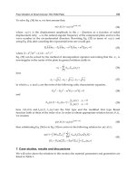
Fig. 11. Free vibration modes of CF rod ( variable cross section uniform rod).


-2
-1.5
-1

-0.5
0
0.5
1
1.5
2
00.20.40.60.81


x/L
Mode Shape Y (x)
i


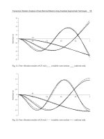
Fig. 12. Free vibration modes of CS rod ( variable cross section uniform rod).
Advances in Vibration Analysis Research

20
3. Conclusion
In this article, some analytical approximation techniques were employed in the transverse
vibration analysis of beams. In a variety of such techniques, the most used ones, namely
ADM, VIM and HPM were chosen for use in the computations. First, a brief theoretical
knowledge was given in the text and then all of the methods were applied to selected cases.
Since the exact values for the free vibration of a uniform beam was available, the analyses
were started for that case. Results showed an excellent agreement with the exact ones that
all three methods were highly effective in the computation of natural frequencies and
vibration mode shapes. Orthogonality of the mode shapes was also proven. Finally, ADM,
VIM and HPM were applied to the free vibration analysis of a rod having variable cross
section. To this aim, a rod with linearly changing radius was chosen and natural frequencies
with their corresponding mode shapes were obtained easily.

The study has shown that ADM, VIM and HPM can be used effectively in the analysis of
vibration problems. It is possible to construct easy-to-use algorithms which are highly
accurate and computationally efficient.
4. References
[1] L. Meirovitch, Fundamentals of Vibrations, International Edition, McGraw-Hill, 2001.
[2] A. Dimarogonas, Vibration for Engineers, 2nd ed., Prentice-Hall, Inc., 1996.
[3] W. Weaver, S.P. Timoshenko, D.H. Young, Vibration Problems in Engineering, 5th ed.,
John Wiley & Sons, Inc., 1990.
[4] W. T. Thomson, Theory of Vibration with Applications, 2nd ed., 1981.
[5] S. S. Rao , Mechanical Vibrations, 3rd ed. Addison-Wesley Publishing Company 1995.
[6] Y. Liu, C. S. Gurram, The use of He’s variational iterationmethod for obtaining the free
vibration of an Euler-Beam beam, Matematical and Computer Modelling, 50( 2009)
1545-1552.
[7] H-L. Lai, J-C., Hsu, C-K. Chen, An innovative eigenvalue problem solver for free
vibration of Euler-Bernoulli beam by using the Adomian Decomposition Method.,
Computers and Mathematics with Applications 56 (2008) 3204-3220.
[8] J-C. Hsu, H-Y Lai,C.K. Chen, Free Vibration of non-uniform Euler-Bernoulli beams with
general elastically end constraints using Adomian modifiad decomposition
method, Journal of Sound and Vibration, 318 (2008) 965-981.
[9] O. O. Ozgumus, M. O. Kaya, Flapwise bending vibration analysis of double tapered
rotating Euler-Bernoulli beam by using the Diferential Transform Method,
Mechanica 41 (2006) 661-670.
[10] J-C. Hsu, H-Y. Lai, C-K. Chen, An innovative eigenvalue problem solver for free
vibration of Timoshenko beams by using the Adomian Decomposition Method,
Journal of Sound and Vibration 325 (2009) 451-470.
[11] S. H. Ho, C. K. Chen, Free transverse vibration of an axially loaded non-uniform
spinning twisted Timoshenko beam using Differential Transform, International
Journal of Mechanical Sciences 48 (2006) 1323-1331.
[12] A.H. Register, A note on the vibrations of generally restrained, end-loaded beams,
Journal of Sound and Vibration 172 (4) (1994) 561_571.

Transverse Vibration Analysis of Euler-Bernoulli Beams Using Analytical Approximate Techniques

21
[13] J.T.S. Wang, C.C. Lin, Dynamic analysis of generally supported beams using Fourier
series, Journal of Sound and Vibration 196 (3) (1996) 285_293.
[14] W. Yeih, J.T. Chen, C.M. Chang, Applications of dual MRM for determining the natural
frequencies and natural modes of an Euler_Bernoulli beam using the singular value
decomposition method, Engineering Analysis with Boundary Elements 23 (1999)
339_360.
[15] H.K. Kim, M.S. Kim, Vibration of beams with generally restrained boundary conditions
using Fourier series, Journal of Sound and Vibration 245 (5) (2001) 771_784.
[16] S. Naguleswaran, Transverse vibration of an uniform Euler_Bernoulli beam under
linearly varying axial force, Journal of Sound and Vibration 275 (2004) 47_57.
[17] C.K. Chen, S. H. Ho, Transverse vibration of rotating twisted Timoshenko beams under
axial loading using differential transform, International Journal of Mechanical
Sciences 41 (1999) 1339- 1356.
[18] C.W. deSilva, Vibration: Fundamentals and Practice, CRC Press, Boca Raton, Florida,
2000.
[19] G. Adomian, Solving Frontier Problems of Physics: The Decomposition Method,
Kluwer, Boston, MA, 1994.
[20] G. Adomian, A review of the decomposition method and some recent results for
nonlinear equation, Math. Comput. Modell., 13(7), 1992, 17-43.
[21] J.H. He, Variational iteration method: a kind of nonlinear analytical technique, Int. J.
Nonlin. Mech., 34, 1999, 699-708.
[22] J.H. He, A coupling method of a homotopy technique and a perturbation technique for
non-linear problems, Int. J. Nonlin. Mech., 35, 2000, 37-43.
[23] J.H. He, An elemantary introduction to the homotopy perturbation method, Computers
and Mathematics with Applications, 57(2009), 410-412.
[24] J.H. He, New interpretation of homotopy perturbation method, International Journal of
Modern Physics B, 20(2006), 2561-2568.

[25] J.H. He, The homotopy perturbation method for solving boundary problems, Phys. Lett.
A, 350 (2006), 87-88.
[26] S.B. Coskun, “Determination of critical buckling loads for Euler columns of variable
flexural stiffness with a continuous elastic restraint using Homotopy Perturbation
Method”, Int. Journal Nonlinear Sci. and Numer. Simulation, 10(2) (2009), 191-197.
[27] S.B Coskun, “Analysis of tilt-buckling of Euler columns with varying flexural stiffness
using homotopy perturbation method”, Mathematical Modelling and Analysis,
15(3), (2010), 275-286.
[28] M.T. Atay, “Determination of critical buckling loads for variable stiffness Euler
Columns using Homotopy Perturbation Method”, Int. Journal Nonlinear Sci. and
Numer. Simulation, 10(2) (2009), 199-206.
[29] B. Öztürk, S.B. Coskun, “The homotopy perturbation method for free vibration analysis
of beam on elastic foundation”, Structural Engineering and Mechanics, An Int.
Journal, 37(4), (2010).
[30] B. Öztürk, “Free vibration analysis of beam on elastic foundation by variational iteration
method“, International journal of Nonlinear Science and Numerical Simulation, 10
(10) 2009, 1255-1262.
Advances in Vibration Analysis Research

22
[31] B. Öztürk, S.B. Coskun, M.Z. Koc, M.T. Atay, Homotopy perturbation method for free
vibration analysis of beams on elastic foundations, IOP Conf. Ser.: Mater. Sci. Engr.,
Volume: 10, Number:1, 9th World Congress on Computational Mechanics and 4th Asian
Pasific Congress on Computational Mechanics, Sydney, Australia (2010).
2
Vibration Analysis of Beams with and without
Cracks Using the Composite Element Model
Z.R. Lu, M. Huang and J.K. Liu
Sun Yat-sen University
P.R. China

1. Introduction
Beams are fundamental models for the structural elements of many engineering applications
and have been studied extensively. There are many examples of structures that may be
modeled with beam-like elements, for instance, long span bridges, tall buildings, and robot
arms.
The vibration of Euler–Bernoulli beams with one step change in cross-section has been well
studied. Jang and Bert (1989) derived the frequency equations for combinations of classical
end supports as fourth order determinants equated to zero. Balasubramanian and
Subramanian (1985) investigated the performance of a four-degree-of-freedom per node
element in the vibration analysis of a stepped cantilever. De Rosa (1994) studied the
vibration of a stepped beam with elastic end supports. Recently, Koplow et al. (2006)
presented closed form solutions for the dynamic response of Euler–Bernoulli beams with
step changes in cross section.
There are also some works on the vibration of beams with more than one step change in
cross-section. Bapat and Bapat (1987) proposed the transfer matrix approach for beams with
n-steps but provided no numerical results. Lee and Bergman (1994) used the dynamic
flexibility method to derive the frequency equation of a beam with n-step changes in cross-
section. Jaworski and Dowell (2008) carried out a study for the free vibration of a
cantilevered beam with multiple steps and compared the results of several theoretical
methods with experiment.
A new method is presented to analyze the free and forced vibrations of beams with either a
single step change or multiple step changes using the composite element method (CEM)
(Zeng, 1998; Lu & Law, 2009). The correctness and accuracy of the proposed method are
verified by some examples in the existing literatures. The presence of cracks in the structural
components, for instance, beams can have a significant influence on the dynamic responses
of the whole structure; it can lead to the catastrophic failure of the structure. To predict the
failure, vibration monitoring can be used to detect changes in the dynamic responses and/or
dynamic characteristics of the structure. Knowledge of the effects of cracks on the vibration
of the structure is of importance. Efficient techniques for the forward analysis of cracked
beams are required. To this end, the composite element method is then extended for free

and forced vibration analysis of cracked beams.
The principal advantage of the proposed method is that it does not need to partition the
stepped beam into uniform beam segments between any two successive discontinuity points
Advances in Vibration Analysis Research

24
and the whole beam can be treated as a uniform beam. Moreover, the presented work can
easily be extended to cracked beams with an arbitrary number of non-uniform segments.
2. Theory
2.1 Introduction to Composite Element Method (CEM)
The composite element is a relatively new tool for finite element modeling. This method is
basically a combination of the conventional finite element method (FEM) and the highly
precise classical theory (CT). In the composite element method, the displacement field is
expressed as the sum of the finite element displacement and the shape functions from the
classical theory. The displacement field of the CEM can be written as

(,) (,) (,)
CEM FEM CT
uxtuxtuxt=+ (1)
where
(,)
FEM
uxt and (,)
CT
uxtare the individual displacement fields from the FEM and CT,
respectively.
Taking a planar beam element as an example, the first term of the CEM displacement field
can be expressed as the product of the shape function vector of the conventional finite
element method
()Nx and the nodal displacement vector q

(,) ()()
FEM
uxtNxqt=
(2)
where
1122
() [ (), (), (), ()]
T
q
tvt tvt t=
θθ
and ‘ v ’ and ‘
θ
’ represent the transverse and rotational
displacements, respectively.
The second term
u
CT
(x,t) is obtained by the multiplication of the analytical mode shapes
with a vector of
N coefficients c ( also called the c degrees-of-freedom or c-coordinates).

1
(,) ()()
N
CT i i
i
uxt xct
=

=
∑
ϕ
(3)
where
i
ϕ
(i=1,2,…N) is the analytical shape function of the beam. Different analytical shape
functions are used according to the boundary conditions of the beam.
Like the FEM, the CEM can be refined using the
h-refinement technique by increasing the
number of finite elements. Moreover, it can also be refined through the
c-refinement
method, by increasing the number of shape functions. Here, we apply the
c-refinement from
the CEM, where the beam needs only to be discretized into one element. This will reduce the
total number of degrees-of-freedom in the FEM.
The displacement field of the CEM for the Euler-Bernoulli beam element can be written
from Equations (1) to (3) as

(,) ()()
CEM
uxtSxQt=
(4)
where
123412
() [ (), (), (), (), (), (), , ()]
N
Sx NxNxNxNx x x x=
φ

φφ
is the generalized shape
function of the CEM,
112212
() [ (), (), (), (), (), (), , ()]
T
N
Qt v t t v t t c t c t c t=
θθ
is the vector of
generalized displacements, and N is the number of shape functions used from the classical
theory.
Vibration Analysis of Beams with and without Cracks Using the Composite Element Model

25
2.2 Vibration analysis for stepped beams without crack
Figure 1 shows the sketch of a beam with n steps, the height of the beam
()dx
with n step
changes in cross section is expressed as

11
21 2
1
0
()
nn n
dxL
dLxL
dx

dL xL
−
≤<
⎧
⎪
≤≤
⎪
=
⎨
⎪
⎪
≤≤
⎩
#
(5)
It is assumed that the beam has aligned neutral axis, the flexibility of the beam
()EI x can be
expressed as

1
2
3
1
3
12
3
1
0
12
()

12
12
n
nn
wd
xL
wd
LxL
EI x
wd
LxL
−
⎧
⎪
≤<
⎪
⎪
⎪
≤≤
=
⎨
⎪
⎪
⎪
⎪
≤≤
⎩
#
(6)
where w is the width of the beam. For the stepped beam with misaligned neutral axes, the

expression of
()EI x can not expressed simply as shown in Equation (6).
The beam mass per unit length is

11
21 2
1
0
()
nn n
wd x L
wd L x L
mx
wd L x L
−
≤<
⎧
⎪
≤≤
⎪
=
⎨
⎪
⎪
≤≤
⎩
#
ρ
ρ
ρ

(7)
where
ρ
is the mass density of the beam.
The elemental stiffness matrix of the stepped beam can be obtained from the following
equation

22
22
0
[][]
()
[][]
T
L
qq qc
cq cc
kk
dS dS
EI x dx
kk
dx dx
⎡
⎤
==
⎢
⎥
⎢
⎥
⎣

⎦
∫
e
K (8)
where the submatrix
[]
qq
k
corresponds to the element stiffness matrix from the FEM for the
stepped beam; the submatrix [ ]
q
c
k corresponds to the coupling terms of the q-dofs and the
c-dofs; submatrix [ ]
c
q
k is a transpose matrix of [ ]
q
c
k , and the submatrix []
cc
k corresponds
to the c-dofs and is a diagonal matrix.
The consistent elemental mass matrix can be expressed as

0
[][]
() ()()
[][]
T

L
qq q
c
c
q
cc
mm
Sx mxSxdx
mm
⎡
⎤
==
⎢
⎥
⎢
⎥
⎣
⎦
∫
e
M
(9)
Advances in Vibration Analysis Research

26
where the submatrix [ ]
qq
m corresponds to the elemental mass matrix from the FEM for the
stepped beam; the submatrix
[]

q
c
m
corresponds to the coupling terms of the q-dofs and the
c-dofs; submatrix [ ]
c
q
m is a transpose matrix of [ ]
q
c
m , and the submatrix []
cc
m corresponds
to the c-dofs and is a diagonal matrix.
After introducing the boundary conditions, this can be performed by setting the associated
degrees-of-freedom in the systematic stiffness matrix
K to be a large number, say,
12
10 , the
governing equation for free vibration of the beam can be expressed as

2
()0V
−
=KM
ω
(10)
where
K and M are system stiffness and mass matrices, respectively,
ω

is the circular
frequency, from which and the natural frequencies are identified. The ith normalized mode
shapes of the stepped beam can be expressed as

4
4
11
N
iiiii
ii
NV V
+
==
Ψ= +
∑∑
ϕ
(11)
The equation of motion of the forced vibration of the beam with n steps when expressed in
terms of the composite element method is
()QQQ
f
t++=MCK
 
(12)
where M and K are the system mass and stiffness matrices, which are the same as those
shown in Equation (10), C is the damping matrix which represents a Rayleigh damping
model,say,
12
aa=+CMK,
1

a and
2
a are constants to be determined from two modal
damping ratios. For an external force F(t) acting at the location
F
x from the left support, the
generalized force vector
()ft
can be expressed as

12341
() () () () () () () ()
T
FFFFFnF
f
tNxNxNxNx x x Ft=
⎡⎤
⎣⎦
"
φφ
(13)
The generalized accelerationQ

, velocity Q

and displacement
Q of the stepped beam can
be obtained from Equation (12) by direct integration. The physical acceleration
(,)uxt


is
obtained from

(,) [()]
T
uxt Sx Q=


(14)
The physical velocity and displacement can be obtained in a similar way, i.e.
(,) [()]
T
uxt Sx Q=


, (15a)
(,) [()]
T
uxt Sx Q= (15b)
2.3 The crack model
Numerous crack models for a cracked beam can be found in the literature. The simplest one
is a reduced stiffness (or increased flexibility) in a finite element to simulate a small crack in
the element (Pandey et al., 1991; Pandy & Biswas, 1994). Another simple approach is to
divide the cracked beam into two beam segments joined by a rotational spring that
Vibration Analysis of Beams with and without Cracks Using the Composite Element Model

27
represents the cracked section (Rizos et al., 1990; Chaudhari & Maiti, 2000). Christides and
Barr (1984) developed the one-dimensional vibration theory for the lateral vibration of a
cracked Euler-Bernoulli beam with one or more pairs of symmetric cracks.

According to Christides and Barr(1984), the variation of bending stiffness
()
d
EI x
along the
cracked beam length takes up the form of

0
()
1( 1)exp(2 /)
d
c
EI
EI x
cxxd
=
+− − −
α
(16)
where E is the Young’s modulus of the beam,
3
0
/12Iwd= is the second moment of area of
the intact beam,
3
1/(1 )
r
cC=−,
/
rc

Cdd=
is the crack depth ratio and
c
d
and d are the
depth of crack and the beam, respectively,
c
x
is the location of the crack.
α
is a constant
which governs the rate of decay and it is estimated by Christides and Barr from experiments
to be 0.667. According to Lu and Law (2009), this parameter needs to be adjusted to be 1.426.
2.4 Vibration analysis for beams with crack(s)
The elemental stiffness matrix of the cracked beam can be obtained from the following
equation

22
22
0
[][]
()
[][]
T
L
qq qc
d
cq cc
kk
dS dS

EI x dx
kk
dx dx
⎡
⎤
==
⎢
⎥
⎢
⎥
⎣
⎦
∫
e
K (17)
It is assumed that the existence of crack does not affect the elemental mass matrix, the
elemental mass matrix can be expressed in the similar way with the intact beam

0
[][]
() ()()
[][]
T
L
qq q
c
c
q
cc
mm

Sx mxSxdx
mm
⎡
⎤
==
⎢
⎥
⎢
⎥
⎣
⎦
∫
e
M (18)
The equation of motion of the forced vibration of a cracked beam with n cracks when
expressed in terms of the composite element method is

11
,,,
( , , , ) ( )
ii nn
Lc Lc Lc
QQ xd xdxdQft++ =MCK
 
(19)
3. Applications Information
3.1 Free and forced vibration analysis for beam without crack
3.1.1 Free vibration analysis for a free-free beam with a single step
The free vibration of the free-free beam studied in Koplow et al. (2006) is restudied using the
CEM and the results are compared with those in Koplow et al. Figure 2 shows the geometry

of the beam under study. The material has a mass density of
3
2830 /kg m=
ρ
, and a Young’s
modulus of 71.7EGPa= . In the CEM when 350 numbers of c-dofs are used, the first three
natural frequencies are converged. The first three natural frequencies of the beam are
291.9Hz, 1176.2Hz and 1795.7Hz, respectively. The calculated natural frequencies from the
CEM are very close to the experimental values in Koplow et al. when the test is measured at
location A in Figure 2, which are 291Hz, 1165Hz and 1771Hz, respectively. The relative
Advances in Vibration Analysis Research

28
errors between the CEM and the experimental values of the three natural frequencies are
0.31%, 0.96% and 1.39%, respectively. This shows the proposed method is accuracte.
3.1.2 Free vibration analysis for a cantilever beam with a several steps
The cantilever beam studied in Jaworski and Dowell (2008) is restudied to further check the
accuracy and effectiveness of the proposed method. Figure 3 shows the dimensions of the
beam under study. The parameters of the beam under study are: 60.6EGPa
=
and
3
2664 /kg m=
ρ
. In the CEM model of the beam, the beam is discretized into one element
and 350 terms of c-dofs are used in the calculation. The first and second flapwise (out-of-
plane) bending mode frequencies are calculated to be 10.758 Hz and 67.553 Hz, and the first
chordwise (in-plane) bending mode frequency is 54.699 Hz. The results from the CEM agree
well with the theoretical results in Jaworski and Dowell using Euler-Bernoulli theory, as
shown in Table 1.

3.1.3 Forced vibration analysis for a cantilever beam with two steps
In this section, the forced vibration analysis for the stepped beam is investigated. The
dynamic responses of the beam under external force are obtained from the CEM and the
results are compared with those from the FEM. Figure 4 shows the cantilever beam under
study. The parameters of the beam under study are 69.6EGPa
=
and
3
2700 /kg m=
ρ
. A
sinusoidal external force is assumed to act at free end of the beam with a magnitude of 1 N
and at a frequency of 10 Hz. The time step is 0.005 second in calculating the dynamic
response. The Rayleigh damping model is adopted in the calculation with 0.01 and 0.02 as
the first two modal damping ratios. In the CEM model, the beam is discretized into one
element and 350 c-dofs are used in the calculation of the dynamic responses. Figure 5 shows
the displacement response, velocity response and acceleration response at the free end of the
beam. In order to check the accuracy of the responses from the CEM, a forced vibration
analysis for the beam is conducted using the FEM. The beam is discretized into 90 Euler-
Bernoulli beam elements with a total of 182 dofs. The corresponding responses from the
FEM and the CEM are compared in Figure 5. This indicates the accuracy of the proposed
method for forced vibration of multiple stepped beam. Figure 6 gives a close view between
the responses from two methods. From this figure, one can see that the two time histories in
every subplot are virtually coincident indicating the excellent agreement between the time
histories.
3.2 Free and forced vibration analysis for beam with crack
3.2.1 Free vibration analysis for a uniform cantilever beam with a single crack
An experimental work in Sinha et al. (2002) is re-examined. The geometric parameters of the
beam are: length 996mm, width 50mm, depth 25mm, material properties of the beam are:
Young’s modulus 69.79EGPa

=
, mass density
3
2600 /kg m=
ρ
. The beam is discretized into
one element and ten shape functions are used in the calculation with the total degrees-of-
freedom in the CEM equals 14, while the total degrees-of-freedom in the finite element
model is 34 for the beam in Sinha et al. The crack depth in the beams varies in three stages of
4mm, 8mm and 12mm. The comparison of predicted natural frequencies of the beam from
the proposed model and those in Sinha et al. and the experimental results are shown in
Table 2. The proposed model, in general, gives better results than the model in Sinha et al.
Vibration Analysis of Beams with and without Cracks Using the Composite Element Model

29
since the latter crack model is a linear approximation of the theoretical crack model of
Christides and Barr.
3.2.2 Free vibration analysis for a cantilever beam with multiple cracks
The last beam above is studied again with a new crack introduced. The first crack is at
595mm from the left end with a fixed crack depth of 12mm while the second crack is at
800mm from the left end with the crack depth varying from 4mm to 12mm in step of 4mm.
Table 3 gives the first five natural frequencies of the beam by CEM method and compares
with those from Sinha et al. and the experimental measurement. The results from CEM are
found closer to the experimental prediction than those in Sinha et al. The above comparisons
show that the CEM approach of modeling a beam with crack(s) is accurate for the vibration
analysis. A significant advantage of the model is the much lesser number of DOFs in the
resulting finite element model of the structure.
3.2.3 Forced vibration analysis for a cracked simply supported beam
The forced vibration analysis for a simply supported cracked beam is conducted in this
section. The effects of the presence of crack on the dynamic response of the beam is

investigated. The parameters of the beam under study are taken as: Young’s
modulus 28E = GPa, width w=200mm, depth d=200mm, length L=8.0m, mass
density
3
2500 /kg m=
ρ
. Two cases are investigated in the following.
Effect of crack depth on the dynamic response
An impulsive force is assumed to act at mid-span of the beam with a magnitude of 100N, the
force starts to act on the beam from the beginning and lasts for 0.1 second. The time step is
0.002 s in calculating the dynamic response. Rayleigh damping model is adopted in the
calculation with 0.01 and 0.02 as the first two modal damping ratios.
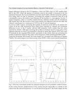
Figure 7 shows comparison on the acceleration response at the 1/4 span of the beam for
different crack depth. The crack is assumed to be at the mid-span of the beam. From this
figure, one can see that the crack depth has significant effect on the dynamic response of the
beam.
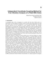
Effect of crack location on the dynamic response
Figure 8 shows comparison on the acceleration response at the 1/4 span of the beam for
different crack locations with a fixed crack depth
/0.3
c
dd
=
. The crack is assumed to be at
the 0.1 L, 0.2L, 0.3L, 0.4L, and 0.5L of the beam. From this figure, one can see that the
response changes with the crack location.
These studies show that the effect of the crack on the dynamic response is significant, so it is
feasible to identify crack from measured structural dynamic responses.
4. Conclusion
The composite element method is proposed for both free and forced vibration analyses of

beams with multiple steps. As the composite beam element is of a one-element-one-member
configuration, modeling with this type of element would not need to take into account the
discontinuity between different parts of the beam. The accuracy of this new composite
element has been compared satisfactorily with existing results. One advantage of the
Advances in Vibration Analysis Research

30
method proposed is that it can be extended easily to deal with beams consisting of an
arbitrary number of non-uniform segments. Regarding the free and forced vibration analysis
for cracked beam using composite element, modelling with this type of element would
allow the automatic inclusion of interaction effect between adjacent local damages in the
finite element model. The accuracy of the present method has been compared satisfactory
with existing model and experimental results.


Fig. 1. Sketch of the stepped free-free beam with n segments


Fig. 2. Sketch of the stepped free-free beam in Koplow et al. (2006). Dimension in millimetre


Fig. 3. Cantilever beam in Jaworski and Dowell (2008) with up and down steps. Dimension
in millimeter
3.175
Vibration Analysis of Beams with and without Cracks Using the Composite Element Model

31

Fig. 4. Sketch of the stepped cantilever beam (dimensions are not scaled)

0 1 2 3 4 5 6 7 8 9 10
-0.03
-0.02
-0.01
0
0.01
0.02
0.03
Time(sec.)
Displ.(m)
0 1 2 3 4 5 6 7 8 9 10
-2
-1
0
1
2
Time(sec.)
Vel.(m/s)
0 1 2 3 4 5 6 7 8 9 10
-150
-100
-50
0
50
100
150
Time(sec.)
Acc.(m/s
2

)

Fig. 5. Forced vibration dynamic response comparison between the CEM and FEM(- Solid:
CEM; Dashed: FEM)
1
10dmm=
2
8dmm=
3
6dmm=
1
300Lmm=
2
300Lmm=
y
x
3
300Lmm=
10bmm
=
Advances in Vibration Analysis Research

32
0 0.1 0.2 0.3 0.4 0.5 0.6 0.7 0.8 0.9 1
-0.03
-0.02
-0.01
0
0.01
0.02

0.03
Time(sec.)
Displ.(m)
0 0.1 0.2 0.3 0.4 0.5 0.6 0.7 0.8 0.9 1
-2
-1
0
1
2
Time(sec.)
Vel.(m/s)
0 0.1 0.2 0.3 0.4 0.5 0.6 0.7 0.8 0.9 1
-150
-100
-50
0
50
100
150
Time(sec.)
Acc.(m/s
2
)

Fig. 6. Forced vibration dynamic response comparison between the CEM and FEM (a close
view; - Solid: CEM, Dashed: FEM)


Fig. 7. Comparison on the dynamic responses for different crack depth
Vibration Analysis of Beams with and without Cracks Using the Composite Element Model

33

Fig. 8. Comparison on the dynamic responses for different crack location

Present Jaworski and Dowell (2008)
CEM Rayleigh-Ritz CMA ANSYS
Mode
Euler Euler Euler Euler
Timoshenk
o
2D Shell 3D Solid
Experiment
1B
ω

10.758 10.752 10.816 10.775 10.745 10.44 10.46 10.63
2B
ω

67.553 67.429 67.463 67.469 67.456 65.54 65.70 66.75
1C
ω

54.699 54.795 54.985 54.469 54.429 49.62 49.83 49.38
Table 1. Natural frequencies [Hz] comparison for the stepped beam in Jaworski and Dowell
(2008)
Note:
1B
ω

,
2B
ω
are the first and second out-of-plane bending mode frequencies,
respectively.
1c
ω
denotes the first in-plane bending mode frequency.
CMA represents component modal analysis.
Advances in Vibration Analysis Research

34



No crack
1
4
c
d
=
mm at
1
595x =
mm
1
8
c
d
=

mm at
1
595x =
mm
1
12
c
d
=
mm at
1
595x =
mm
Mod
e
Exp.
Propos
ed
Exp.
Sinha et
al.(2002)
Propos
ed
Exp.
Sinha et
al.(2002)
Propose
d
Exp.
Sinha et

al.(2002)
Propos
ed
1 40.000 39.770 39.688 39.379 39.490 39.375 39.094 39.242 39.063 38.857 38.869
2 109.688 109.340 109.063 108.206 108.633 108.125 107.132 107.670 105.938 106.278 106.293
3 215.000 214.795 215.000 214.087 214.230 214.688 213.825 213.986 214.375 213.622 213.631
4 355.000 354.853 354.688 353.107 353.683 353.438 351.872 352.524 350.625 350.881 350.921
5 528.750 529.601 527.188 524.696 526.540 522.812 520.452 522.448 513.125 517.219 517.003

Table 2. Comparison of natural frequencies (Hz) of the aluminium free-free beam with one
crack in Sinha et al.(2002)



No crack
1
12
c
d = mm at
1
595x
=
mm
2
4
c
d
=
mm at
2

800x
=
mm
1
12
c
d = mm at
1
595x
=
mm
2
8
c
d
=
mm at
2
800x
=
mm
1
12
c
d = mm at
1
595x
=
mm
2

12
c
d = mm at
2
800x
=
mm
Mod
e
Exp.
Propos
ed
Exp.
Sinha et
al.(2002)
Propos
ed
Exp.
Sinha et
al.(2002)
Propose
d
Exp.
Sinha et
al.(2002)
Propose
d
1 40.000 39.770 38.750 38.352 38.607 38.437 37.897 38.246 37.500 37.513 37.703
2 109.688 109.340 105.938 105.890 106.196 105.938 105.510 106.062 105.625 105.559 105.858
3 215.000 214.795 213.750 212.207 212.786 212.813 210.897 211.643 210.000 209.815 209.975

4 355.000 354.853 350.000 348.920 349.843 349.063 347.235 348.410 345.625 345.876 346.374
5 528.750 529.601 512.500 514.575 514.735 511.250 512.903 513.044 507.500 510.560 510.633

Table 3. Comparison of natural frequencies (Hz) of the aluminium free-free beam with two
cracks in Sinha et al.(2002)
Vibration Analysis of Beams with and without Cracks Using the Composite Element Model

35
5. References
Balasubramanian T.S. & Subramanian G. (1985). On the performance of a four-degree-of-
freedom per node element for stepped beam analysis and higher
frequency estimation. Journal of Sound and Vibration, Vol.99, No.4, 563–567, ISSN:
0022-460X.
Bapat C.N & Bapat C. (1987). Natural frequencies of a beam with non-classical boundary
conditions and concentrated masses. Journal of Sound and Vibration, Vol.112, No.1,
177–182, ISSN: 0022-460X.
Chaudhari T.D & Maiti S.K. (2000). A study of vibration geometrically segmented beams
with and without crack. International Journal of Solids and Structures, Vol. 37, 761-779,
ISSN: 0020-7683.
Christides A. & Barr A.D.S. (1984). One dimensional theory of cracked Bernoulli-Euler
beams. International Journal of Mechanical Science, Vol. 26, 639-648, ISSN:
0020-7403.
De Rosa M.A. (1994). Free vibration of stepped beams with elastic ends. Journal of Sound and
Vibration, Vol.173, No.4, 557–563, ISSN: 0022-460X.
Jang S.K. & Bert C.W. (1989). Free vibrations of stepped beams: exact and
numerical solutions. Journal of Sound and Vibration, Vol. 130, No.2, 342–346, ISSN:
0022-460X.
Jaworski J.W. & Dowell E.H. (2008). Free vibration of a cantilevered beam with multiple
steps: Comparison of several theoretical methods with experiment. Journal of Sound
and Vibration, Vol.312, No. 4-5, 713-725, ISSN: 0022-460X.

Lee J. & Bergman L.A. (1994). Vibration of stepped beams and rectangular plates by an
elemental dynamic flexibility method. Journal of Sound and Vibration, Vol. 171, No.5,
617–640, ISSN: 0022-460X.
Lu Z.R. & Law S.S. (2009). Dynamic condition assessment of a cracked beam with the
composite element model. Mechanical Systems and Signal Processing, Vol. 23, No. 3,
415-431, ISSN: 0888-3270.
Michael A. Koplow, Abhijit Bhattacharyya and Brian P. Mann. (2006). Closed form solutions
for the dynamic response of
Euler–Bernoulli beams with step changes in cross
section. Journal of Sound and Vibration, Vol.295, No.1-2, 214-225, ISSN: 0022-460X.
Pandey A.K., Biswas M. & Samman M.M. (1991). Damage detection from change in
curvature mode shapes. Journal of Sound and Vibration, Vol.145, 321-332, ISSN: 0022-
460X.
Pandey A.K & Biswas M. (1994). Damage detection in structures using change in flexibility.
Journal of Sound and Vibration, Vol.169, 3-17, ISSN: 0022-460X.
Rizos P.F; Aspragathos N. & Dimarogonas A.D. (1990). Identification of crack location and
magnitude in a cantilever beam. Journal of Sound and Vibration, Vol.138, 381-388,
ISSN: 0022-460X.
Sinha J.K; Friswell M.I & Edwards S. (2002). Simplified models for the location of cracks in
beam structures using measured vibration data. Journal of Sound and Vibration, Vol.
251, No.1, 13-38, ISSN: 0022-460X.
Advances in Vibration Analysis Research

36
Zeng P. (1998). Composite element method for vibration analysis of structure, Part II:
1
C
Element (Beam). Journal of Sound and Vibration, Vol. 218, No.4, 658-696, ISSN:
0022-460X.
3

Free Vibration Analysis of Curved
Sandwich Beams: A Dynamic Finite Element
Seyed M. Hashemi and Ernest J. Adique
Ryerson University
Canada
1. Introduction
Applications of sandwich construction and composites continue to expand. They are used in
a number of industries such as the aerospace, automotive, marine and even sports
equipment. Sandwich construction offers designers high strength to weight ratios, as well as
good buckling resistance, formability to complex shapes and easy reparability, which are of
extremely high importance in aerospace applications. Due to their many advantages over
traditional aerospace materials, the analysis of sandwich beams has been investigated by a
large number of authors for more than four decades. Sandwich construction can also offer
energy and vibration damping when a visco-elastic core layer is used. However, such non-
conservative systems are not the focus of the present study.
The most common sandwich structure is composed of two thin face sheets with a thicker
lightweight, low-stiffness core. Common materials used for the face layers are metals and
composite while the core is often made of foam or a honeycomb structure made of metal. It
is very important that the core, although weaker than the face layers, be strong enough to
resist crushing. The current trend in the aerospace industry of using composites and
sandwich material, to lighten aircraft in an attempt to make them more fuel efficient, has led
to further recent researches on development of reliable methods to predict the vibration
behaviour of sandwich structures.
In the late 1960s, pioneering works in the field of vibration analysis of viscously damped
sandwich beams (Di Taranto, 1965, and Mead and Marcus, 1968) used classical methods to
solve the governing differential equations of motion, leading to the natural frequencies and
mode shapes of the system. Ahmed (1971) applied the finite element method (FEM) to a
curved sandwich beam with an elastic core and performed a comparative study of several
different formulations in order to compare their performances in determining the natural
frequencies and mode shapes for various different beam configurations. Interest in the

vibration behaviour of sandwich beams has seen resurgence in the past decade with the
availability of more powerful computing systems. This has allowed for more complex finite
element models to be developed. Sainsbury and Zhang (1999), Baber et al. (1998), and
Fasana and Marchesiello (2001) are just some among many researchers who investigated
FEM application in the analysis of visco-elastically damped sandwich beams. The Dynamic
Stiffness Method (DSM), which employs symbolic computation to combine all the governing
differential equations of motion into a single ordinary differential equation, has also been
well established. Banerjee and his co-workers (1995-2007) and Howson and Zare (2005) have
Advances in Vibration Analysis Research

38
published numerous papers on DSM illustrating its successful application to numerous
homogeneous and sandwich/composite beam configurations, with a number of papers
focusing on elastic-core sandwich beams. It is worth noting that in all the above-mentioned
sandwich element models, the beam motion is assumed to exhibit coupled bending-axial
motion only, with no torsional or out-of-plane motion. Also, the layers are assumed to be
perfectly and rigidly joined together and the interaction of the different materials at the
interfaces is ignored. Although it is known that bonding such very much different materials
will cause stress at the interfaces, the study of their interactions and behaviour at the
bonding site is another research topic altogether and is beyond the scope of the present
Chapter.
Another important factor that largely affects the results of the sandwich beam analysis is the
assumed vibration behaviour of the layers. The simplest sandwich beam model utilizes
Euler-Bernoulli theory for the face layers and only allows the core to deform only in shear.
This assumption has been widely used in several DSM and FEM studies such as those by
Banerjee (2003), Ahmed (1971,1972), Mead and Markus (1968), Fasana and Marchesiello
(2001), Baber et al. (1998), and in earlier papers by the authors; see e.g., Adique & Hashemi
(2007), and Hashemi & Adique (2009). In more recent publications, Banerjee derived two
new DSM models which exploit more complex displacement fields. In the first and simpler
of the two (Banerjee & Sobey, 2005), the core bending is governed by Timoshenko beam

theory, whereas the face plates are modeled as Rayleigh beams. To the authors’ best
knowledge, the most comprehensive sandwich beam theory was developed and used by
Banerjee et al. (2007), where all three layers are modeled as Timoshenko beams. However,
increasing the complexity of the model also significantly increases the amount of numerical
and symbolic computation in order to achieve the complete formulation.
Classical FEM method has a proven track record and is the most commonly used method for
structural analysis. It is a systematic approach, leading to element stiffness and mass
matrices, easily adaptable to a wide range of problems. The polynomial shape functions are
used to approximate the displacement fields, resulting in a linear eigenproblem, whose
solutions are the natural frequencies of the system. Most commercial FEM-based structural
analysis software also offer multi-layered elements that can be used to model layered
composite materials and sandwich construction (e.g., ANSYS
®
and MSC
NASTRAN/PATRAN
®
). As a numerical formulation, however, the versatility of the FEM
theory comes with a drawback; the accuracy of its results depends on the number of
elements used in the model. This is the most evident when FEM is used to evaluate system
behaviour at higher frequencies, where a large number of elements are needed to achieve
accurate results.
Dynamic Stiffness Matrix (DSM) method, on the other hand, provides an analytical solution
to the free vibration problem, achieved by combining the coupled governing differential
equations of motion of the system into a single higher order ordinary differential equation.
Enforcing the boundary conditions then leads to the system’s DSM and the most general
closed form solution is then sought. The DSM formulation results in a non-linear eigenvalue
problem and the bi-section method, combined with the root counting algorithm developed
by Wittrick & Williams (1971), is then used as a solution technique. DSM provides exact
results (i.e., closed form solution) for any of the natural frequencies of the beam, or beam-
structure, with the use of a single continuous element characterized by an infinite number of

degrees of freedom. However, the DSM methods is limited to special cases, for which the
closed form solution of the governing differential equation is known; e.g., systems with
Free Vibration Analysis of Curved Sandwich Beams: A Dynamic Finite Element

39
constant geometric and material properties and only a certain number of boundary
conditions.
The Dynamic Finite Element (DFE) method is a hybrid formulation that blends the well-
established classical FEM with the DSM theory in order to achieve a model that possesses all
the best traits of both methods, while trying to minimize the effects of their limitations; i.e.,
to fuse the adaptability of classical FEM with the accuracy of DSM. Therefore, the
approximation space is defined using frequency dependent trigonometric basis functions to
obtain the appropriate interpolation functions with constant parameters over the length of
the element. DFE theory was first developed by Hashemi (1998), and its application has ever
since been extended by him and his coworkers to the vibration analysis of intact (Hashemi
et al.,1999, and Hashemi & Richard, 2000a,b) and defective homogeneous (Hashemi et al.,
2008), sandwich (Adique & Hashemi, 2007-2009, and Hashemi & Adique, 2009, 2010) and
laminated composite beam configurations (Hashemi & Borneman, 2005, 2004, and Hashemi
& Roach, 2008a,b) exhibiting diverse geometric and material couplings. DFE follows a very
similar procedure as FEM by first applying the weighted residual method to the differential
equations of motion. Next, the element stiffness matrices are derived by discretizing the
integral form of the equations of motion. For FEM, the polynomial interpolation functions
are used to express the field variables, which in turn are introduced into the integral form of
the equations of motion and the integrations are carried out and evaluated in order to obtain
the element matrices. At this point, DFE applies an additional set of integration by parts to
the element equations, introduces the Dynamic Trigonometric Shape Functions (DTSFs),
and then carries out the integrations to form the element matrices. In the case of a three-
layered sandwich beam, the closed form solutions to the uncoupled parts of the equations of
motion are used as the basis functions of the approximation space to develop the DTSFs.
The assembly of the global stiffness matrix from the element matrices follows the same

procedure for FEM, DSM and DFE methods. Like DSM, the DFE results in a non-linear
eigenvalue problem, however, unlike DSM, it is not limited to uniform/stepped geometry
and can be readily extended to beam configurations with variable material and geometric
parameters; see e.g., Hashemi (1998).
In the this Chapter, we derive a DFE formulation for the free vibration analysis of curved
sandwich beams and test it against FEM and DSM to show that DFE is another viable tool
for structural vibration analysis. The face layers are assumed to behave according to Euler-
Bernoulli theory and the core deforms in shear only, as was also studied by Ahmed
(1971,1972). The authors have previously developed DFE models for two straight, 3-layered,
sandwich beam configurations; a symmetric sandwich beam, where the face layers are
assumed to follow Euler-Bernoulli theory and core is allowed to deform in shear only
(Adique & Hashemi, 2007, and Hashemi & Adique, 2009), and a more general non-
symmetric model, where the core layer of the beam behaves according to Timoshenko
theory while the faces adhere to Rayleigh beam theory (Adique & Hashemi, 2008, 2009). The
latter model not only can analyze sandwich beams, where all three layers possess widely
different material and geometric properties, but also it has shown to be a quasi-exact
formulation (Hashemi & Adique, 2010) when the core is made of a soft material.
2. Mathematical model
Figure 1 below shows the notation and corresponding coordinate system used for a
symmetrical curved three-layered sandwich beam with a length of S and radius R at the
Advances in Vibration Analysis Research

40
mid-plane of the beam. The thicknesses of the inner and outer face layers are t while the
thickness of the core is represented by t
c
. In the coordinate system shown, the z-axis is the
normal co-ordinate measured from the centre of each layer and the y-axis is the
circumferential coordinate and coincides with the centreline of the beam. The beam only
deflects in the y-z plane. The top and bottom faces, in this case, are modelled as Euler-

Bernoulli beams, while the core is assumed to have only shear rigidity (e.g., the stresses in
the core in the longitudinal direction are zero). The centreline displacements of layers 1 and
3 are v
1
and v
2
, respectively. The main focus of the model is flexural vibration, w, and is
common among all three layers, which leads to the assumption v
1
= -v
2
= -v.


Fig. 1. Coordinate system and notation for curved symmetric three-layered sandwich beams
For the beam model developed, the following assumptions made (Ahmed, 1971):
• All displacements and strains are so small that the theory of linear elasticity still applies.
• The face materials are homogeneous and elastic, while the core material is assumed to
be homogeneous, orthotropic and rigid in the z-direction.
• The transverse displacement w does not vary throughout the thickness of the beam.
• The shear within the faces is negligible.
• The bending strain within the core is negligible.
• There is no slippage or delamination between the layers during deformation.
Using the model and assumptions described above, Ahmed (1971) used the principle of
minimum potential energy to obtain the differential equations of motion and corresponding
boundary conditions. For free vibration analysis, the assumption of simple harmonic motion
is used, leading to the following form of the differential equations of motion for a curved
symmetrical sandwich beam (Ahmed, 1971):
Free Vibration Analysis of Curved Sandwich Beams: A Dynamic Finite Element

41

22
22
1
22 2
12
(4) 0,
vhw
Qv
y
y
β
ωβ
αα
∂∂
+
−− =
∂
∂
(1)

4222 2 2
2
2
42222 2
12
() 0,
wh w h v
Qw

y
yyR
βα β
ω
γγ γ
∂∂ ∂
−
+− − =
∂
∂∂
(2)
where

22 223
12
2 , (1 / /4 ) , /6,
, 2 /3, 2 .
cc c
c
f
cc
f
cc
Et t t R G Et
htt Q t t Q t t
αβ γ
ρ
ρρρ
==+ =
=+ =+ =+

(3)
In the equations above, v(y) and w(y) are the amplitudes of the sinusoidally varying
circumferential and radial displacements, respectively. E is the Young’s modulus of the face
layers, G
c
is the shear modulus of the core layer, and ρ and ρ
c
are the mass densities of the
face and core materials, respectively. The appropriate boundary conditions are imposed at
y=0 and y=S. For example, for
•
clamped at y = 0 and y = S; v = w = ∂w/∂y = 0.
•
simply supported at y = 0 and y = S; ∂v/∂y = w = ∂
2
w/∂y
2
= 0.
•
cantilever configuration; at y = 0: v=w=∂w/∂y=0; and at y=S: ∂v/∂y=∂
2
w/∂y
2
=0 and a
resultant force term of
γβ
∂
∂+ +∂ ∂ =
23 3 2
[2 / 2 (2 / )] 0wy hvhwy , …

For harmonic oscillation, the weak form of the governing equations (1) and (2) are obtained
by applying a Galerkin-type integral formulation, based on the weighted-residual method.
The method involves the use of integration by parts on different elements of the governing
differential equations and then the discretization of the beam length into a number of two-
node beam elements (Figure 2).


Fig. 2. Domain discretized by N number of 2-noded elements
Applying the appropriate number of integration by parts to the governing equations and
discretization lead to the following form (in the equations below, primes denote integration
with respect to y):

δα δω β δ β
=−−+
∫∫ ∫
222 2
1
00 0
'' ( 4) 2 '
ll l
k
v
W v v dy v Q vdy v h w dy
(4)

δγ δ β δα ω δ β
=+ +−+
∫∫ ∫ ∫
222222 2
2

00 0 0
"" ' ' (/ ) '2
ll l l
k
w
W w w dy w h w dy w R Q wdy w h vdy (5)
All of the resulting global boundary terms produced by integration by parts before
discretization in the equations above are equal to zero. The above equations are known as
the element Galerkin-type weak form associated to the discretized equations (4) and ( 5) and
also satisfy the principle of virtual work:
Advances in Vibration Analysis Research

42

=
−=+−=() 0
INT EXT v w EXT
WW W W W W (6)
For the free vibration analysis, W
EXT
= 0, and

Number of Elements
1
; where
kkkk
INT v w
k
WWWWW
=

==+
∑
(7)
In the equations above, δv and δw are the test- or weighting -functions, both defined in the
same approximation spaces as v and w, respectively. Each element is defined by nodes j and
j+1 with the corresponding co-ordinates (l=x
j+1
–x
j
). The admissibility condition for finite
element approximation is controlled by the undiscretized forms of equations (4) and (5).
3. Finite elements method (FEM) derivations
Two different FEM models were derived for the curved beam model. The first one has three
degrees of freedom (DOFs) per node and uses a linear approximation for the axial
displacement and a Hermite type polynomial approximation for the bending displacement.

+
+
=
<> = +
11 2 1
() () { } () ()
v
jj
v
j
v
j
v
y

N
y
vv N
y
vN
y
v (8)
+
+++
=< > = + + +
11 1 2 3 14 1
() () { ' ' } () () ' () () '
w
jjj j
w
j
w
j
w
j
w
j
wy Ny w w w w N yw N yw N yw N yw (9)
In the equations above, v
j
, v
j+1
, w
j
and w

j+1
are the nodal values at j and j+1 corresponding to
the circumferential and radial displacements, respectively (these can be likened to the axial
and flexural displacements for a straight beam). w
j
’ and w’
j+1
represent the nodal values of
the rate of change of the radial displacements with respect to x (which can be likened to the
bending slope for a straight beam). The same approximations were also used for δv and δw,
respectively. The first FEM formulation is achieved when the nodal approximations
expressed by equations (8) and (9) are applied to simplify equations (4) and (5). Similar
approximations are also used for the corresponding test functions, δv and δw, and the
integrations are performed to arrive at the classical linear (in ω
2
) eigenvalue problem as
functions of constant mass and stiffness matrices, which can be solved using programs such
as Matlab
®
.
In the second FEM model the number of DOFs per node is increased to four and Hermite-
type polynomial approximations are used for both the axial and bending displacements.

+
++++
=< > = + + +
11 1 2 13 1 4 1
() () { ' ' } () ()' () ()'
v
jjj j

v
j
v
j
v
j
v
j
v
y
N
y
vv v v N
y
vN
y
vN
y
vN
y
v (10)

+
+++
=< > = + + +
11 1 2 3 14 1
() () { ' ' } () () ' () () '
w
jjj j
w

j
w
j
w
j
w
j
wy Ny w w w w N yw N yw N yw N yw (11)
In the equations above, v
j
, v
j+1
, w
j
and w
j+1
are the nodal values at j and j+1 corresponding to
the circumferential and radial displacements, respectively. v
j
’, v’
j+1
, w
j
’ and w’
j+1
are the
nodal values at j and j+1 for the rate of change with respect to y for the circumferential and
radial displacements, respectively. The same approximations are also used for δv and δw.
The second FEM formulation applies equations (10) and (11) to simplify equations (4) and
(5) to produce the linear (in ω

2
) eigenvalue problem as a function of constant mass and
stiffness matrices, which can again be solved using programs such as Matlab
®
. For the
current research, both FEM models were programmed using Matlab
®
.
Free Vibration Analysis of Curved Sandwich Beams: A Dynamic Finite Element

43
4. Dynamic finite element (DFE) formulation
In order to obtain the DFE formulation, an additional set of integration by parts are applied
to the element equations (4) and (5) leading to:

δα δω δ β δα δ β
×
=− + + + +
∫∫ ∫
 


24
22 2 2 2
10
00 0
(*) [ ] Coupling
[] Uncoupled
(" ) (4) [' ] (2 )'
k

VW
V
ll l
k l
V
k
k
W v v Q vdy v vdy v v v h w dy (12)

222222
1
0
(**)
22 2 2
000
[] Uncoupled
("" " (/ ))
[ ' ] [ " '] [ "' ]
k
W
l
k
W
lll
k
Ww whwRQwdy
wh w w w w w w
δγδ βδα ω
δβ δγ δγ δ
=−+ − +

+− +
∫


42
2
0
[] Coupling
'(2 )
WV
l
k
h vdy
β
×
∫


(13)
Equation (12) and (13) are simply a different, yet equivalent, way of evaluating equations (4)
and (5) at the element level. The follwing non-nodal approximations are defined

δ
δ
=
<> =<>() { }; () {};
VV
vPy avPy a (14)

δδ

=< > =< >() { }; () {},
WV
wPy bwPy b
(15)
where {a} and {b} are the generalized co-ordinates for v and w, respectively, with the basis
functions of approximation space expressed as:

ε
εε
<>=( ) cos( ) sin( )/ ;
V
Py y y
(16)

σ
τσ τσ
σ
σστ στ
−
−
<>=
++
22 33
sin( ) cosh( ) cos( ) sinh( ) sin( )
() cos( ) ,
W
yyyyy
Py y
(17)
where ε, σ and τ (shown below) are calculated based on the characteristic equations (*) and

(**) in expressions (12) and (13) being reduced to zero.

ββγαω
ω
εστ
α
γ
±− −
=
22 222 2 2 2 2
2
2
1
2
2
h(h)4(/ )
; , =
2
RQ
Q
(18)
The non-nodal approximations (14) and (15) are made for δv, v, δw and w so that the integral
terms (*) and (**) in expressions (12) and (13) become zero. The former term has a 2
nd
-order
characteristic equation of the form A
1
D
2
+ B

1
ω
2
= 0, whereas the latter one has a 4
th
-order
characteristic equation of the form A
2
D
4
– B
2
D
2
+ C
2
ω
2
= 0. Solving (*) and (**) yields the
solution to the uncoupled parts of (12) and (13), which are subsequently used as the
dynamic basis functions of approximation space to derive the DTSFs. The nodal
approximations for element variables, v(y) and w(y), are then written as:
=< > < >
-1
nV nV 1 2
( ) [P ] {u } = ( ) { };
VV
vPy Ny vv (19)
=< > < >
-1

nW nW 1 1 2 2
( ) [P ] {u } = ( ) { ' ' };
VW
wPy Ny wwww (20)