Advances in Flight Control Systems Part 10 docx

Fault-Tolerance of a Transport Aircraft with Adaptive Control and Optimal Command Allocation

167
health. These features make the proposed control architecture very appealing for
reconfiguration purposes.
5. Numerical validation
The FCS has been applied in a case study with a large transport aircraft. The works has been
performed within the GARTEUR Action Group 16, project focused on Fault-Tolerant
Control. In that project a benchmark environment (Smaili et al., 2006) has been developed
modelling a bunch of surface actuators faulty conditions. A brief summary of all these
conditions is given in Table 3, while a detailed explanation of the benchmark can be found
in (Smaili et al., 2006).
Several manoeuvres are considered in the benchmark to be accomplished in the various
faulty conditions. The test results are here shown both in terms of time histories of the state
variables and with a visual representation of the trajectories performed by the airplane.

Stuck Ailerons:

Both inboard and outboard ailerons are stuck.

Stuck Elevators:
Both inboard and outboard elevators are stuck.

Stabilizer Runaway
:
The stabilizer goes at the maximum speed toward
the maximum deflection.

Rudder Runaway
:
The upper and lower rudders go at the maximum

speed toward the maximum deflection.

Loss of Vertical Tail
:
The vertical tail separates from the aircraft.



Table 3. Failures considered in the test campaign
Only the most meaningful conditions are here reported and discussed. To better
demonstrate the improvement of fault-tolerance achieved by adopting the adaptive control
in conjunction with the Control Allocation, comparison is made between three versions of
the FCS, the first is a baseline SCAS developed with classic control techniques. The two
remaining FCS are based on the adaptive SCAS with and without the CA respectively. As
above said, only limited FD information are supposed to be provided, that is, the
information about whether an actuator is failed or not but the current position of the failed
actuator will be considered as unknown. The CA parameters have been set to:

33
33
6
10
×
×
=
=
=
IW
IW
v

u
γ
(22)
Advances in Flight Control Systems

168
5.1 Straight flight with stabilizer failure
In this condition, while in straight and levelled flight, the aircraft experiences a stabilizer
runaway to maximum defection that generates a pitching down moment. The initial flight
condition data are summarized in Table 4.

Altitude
[m]
True Airspeed
[m/s]
Heading
[deg]
Mass
[kg]
Flaps
[deg]
600 92.6 180 263,000 20
Table 4. Flight condition data


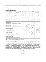
(a) Trajectories

(b) Time plots
Fig. 3. Straight flight with stabilizer runaway with classic technique (dotted line), DAMF
(solid line) and DAMF+CA (dashed line)

Fig. 3 (a) shows the great improvement achieved thanks to the adoption of the control
allocation. Note that the classic technique, for this failure condition, shows adequate
robustness. This is caused by its structure. In fact, the longitudinal control channel (PI for
Fault-Tolerance of a Transport Aircraft with Adaptive Control and Optimal Command Allocation

169
pitch-angle above proportional pitch-rate SAS) affects only the elevators, while the stabilizer is
supposed to be operated by the pilot separately. In this way, the stabilizer runway results to be
a strong, but manageable disturbance. Instead, the DAMF tries to recover the attitude
lavishing stronger control effort on the faulty stabilizer, the most effective surface, with bad
results. The awareness of the fault on the stabilizer gives the chance to the CA technique to
compensate by moving the control effort from this surface to the elevators, thus achieving the
same results of the classical technique. As it is also evident in the time plots of Fig. 3 (b) when
the failure is detected and isolated (here it is supposed to be done in 10 sec after the failure
occurs), the aircraft recovers a more adequate attitude to carry out properly the manoeuvre.

5.2 Right turn and localizer intercept with rudder runaway
This manoeuvre consists in the interception of the localizer beam, parallel to initial flight
path, but opposite in versus. So, in the early stage of the manoeuvre, a right turn is
performed, and then the capture and the tracking of the localizer beam are carried out. The
fault, instead, consists in a runaway of both upper and lower rudder surfaces, so giving a
strong yawing moment opposite to the desired turn. The initial flight condition data are
summarized in Table 4.
In this failure case, a classical technique is totally inadequate to face such a failure, so
leading the aircraft to crash into the ground. Instead, the DAMF shows to be robust enough
to deal with this failure condition and it makes the aircraft to accomplish the manoeuvre,
even though with reduced performance. The control allocation technique, instead, shows a
sensible improvement of the robustness (see Fig. 4), if compared to the DAMF technique.
The awareness of the fault (detected 10 sec after it actually occurs) allows the control laws to
fully exploit all the efficient effectors, thus accomplishing the manoeuvre smoothly. It is

worth noting that in this case the DAMF without CA is robust enough to accomplish the
manoeuvre, even though with degraded performances.
5.3 Right turn and localizer intercept with loss of vertical tail
The manoeuvre, here considered, is the same described in the previous subsection, but the
failure scenario consists in the loss of the vertical tail (Smaili et al., 2006). The initial flight
condition data are summarized in Table 4. This is both a structural and actuation failure, in
fact, the loss of the rudders strongly affects the lateral-directional aerodynamics and stability,
compromising the possibility to damp the rotations about the roll and yaw axes. In this case
(see Fig. 5), the classical technique is not able to reach lateral stability. Instead, no significant
differences are evidenced between the two versions of the adaptive FCS (with and without
CA). In fact, the information about the efficiency of the differential thrust is already available
to the DAMF, due to the linear model of the bare Aircraft. Thus, as the tracking errors increase,
the core control laws raise the control effort for both the rudders (failed) and the differential
thrust. The latter is efficient enough to ensure the manoeuvrability.
6. Conclusions
In this chapter a fault-tolerant FCS architecture has been proposed. It exploits the main
features of two different techniques, the adaptive control and the control allocation. The
contemporaneous usage of these two techniques, the former for the robustness, and the
latter for the explicit actuators failure treatment, has shown significant improvements in
terms of fault-tolerance if compared to a simple classical controller and to the only adaptive

Advances in Flight Control Systems

170



(a) Trajectories

(b) Time plots
Fig. 4. Right turn and localizer intercept with rudder runaway with classic technique (dotted
line), DAMF (solid line) and DAMF+CA (dashed line)
Fault-Tolerance of a Transport Aircraft with Adaptive Control and Optimal Command Allocation

171



(a) Trajectories


(b) Time plots
Fig. 5. Loss of vertical tail failure scenario, while performing a right turn & localizer intercept
runaway with classic technique (dotted line), DAMF (solid line) and DAMF+CA (dashed line)
Advances in Flight Control Systems

172
controller. The ability of the DAMF to on-line re-compute the control gains guarantees both
robustness and performance, as shown in the proposed test cases. However, the
contemporary usage of a control allocation scheme allowed improving significantly the
fault-tolerance capabilities, at the only expense of requiring some limited information about
the vehicle actuators’ health. Therefore the proposed fault-tolerant scheme appears to be
very promising to deal with drastic off-nominal conditions as the ones induced by severe
actuators failure and damages thus improving the overall adaptive capabilities of a
reconfigurable flight control system.
7. References
Bodson, M. & Groszkiewicz, J. E. (1997). Multivariable Adaptive Algorithms for
Reconfigurable Flight Control, IEEE Transaction on Control Systems Technology, Vol.

5, No. 2, pp. 217-229.
Boskovic, J. D. & Mehra, R. K. (2002), Multiple-Model Adaptive Flight Control Scheme for
Accommodation of Actuator Failures, Journal of Guidance, Control, and Dynamics,
Vol. 25, No. 4, pp. 712-724.
Buffington, J. & Chandler, P. (1998), Integration of on-line system identification and
optimization-based control allocation, Proceedings of AIAA Guidance, Navigation, and
Control Conference and Exhibit, Boston, MA.
Burken, J. J., Lu, P., Wu, Z. & Bahm, C. (2001), Two Reconfigurable Flight-Control Design
Methods: Robust Servomechanism and Control Allocation, Journal of Guidance,
Control, and Dynamics, Vol. 24, No. 3, pp. 482-493.
Calise, A. J., Hovakimyan, N. & Idan, M. (2001). Adaptive output feedback control of
nonlinear systems using neural networks, Automatica, Vol. 37, No. 8, pp. 1201–1211.
Durham, W. C. & Bordignon, K. A. (1995), Closed-Form Solutions to Constrained Control
Allocation Problem, Journal of Guidance, Control and Dynamics, Vol. 18, No. 5, pp.
1000-1007.
Enns, D. (1998), Control Allocation Approaches, Proceedings of the AIAA Guidance, Navigation
and Control Conference, Boston, MA.
Harkegard, O. (2002), Efficient Active Set Algorithms for Solving Constrained Least squares
Problems in Aircraft Control Allocation, Proceedings. of the 41
st
IEEE Conference on
Decision and Control, Vol. 2, pp. 1295-1300.
Kim, K. S., Lee, K. J. & Kim, Y. (2003), Reconfigurable Flight Control System Design Using Direct
Adaptive Method, Journal of Guidance, Control, and Dynamics, Vol. 26, No. 4, pp. 543-550.
Luenberger, D. G. (1989), Linear and Nonlinear Programming, 2
nd
ed., Addison-Welsey, 1989,
Chapter 11.
Patton, R. J. (1997). Fault-Tolerant Control Systems: The 1997 Situation, Proceedings of the
IFAC Symposium on Fault Detection, Supervision and Safety for Technical Processes, Vol.

2, pp. 1033–1055.
Smaili, M. H., Breeman, J., Lombaerts, T. J. & Joosten, D. A. (2006), A Simulation Benchmark
for Integrated Fault Tolerant Flight Control Evaluation, Proceedings of AIAA
Modeling and Simulation Technologies Conference and Exhibit, Keystone, CO.
Tandale, M. & Valasek, J. (2003), Structured Adaptive Model Inversion Control to
Simultaneously Handle Actuator failure and Actuator Saturation, Proceedings. of the
AIAA Guidance, Navigation and Control Conference, Austin, TX.
Virnig, J. & Bodden, D. (2000), Multivariable Control Allocation and Control Law
Conditioning when Control Effector Limit, Proceedings of the AIAA Guidance,
Navigation and Control Conference, Denver, CO.
9
Acceleration-based 3D Flight Control for UAVs:
Strategy and Longitudinal Design
Iain K. Peddle and Thomas Jones
Stellenbosch University
South Africa
1. Introduction
The design of autopilots for conventional flight of UAVs is a mature field of research. Most
of the published design strategies involve linearization about a trim flight condition and the
use of basic steady state kinematic relationships to simplify control law design (Blakelock,
1991);(Bryson, 1994). To ensure stability this class of controllers typically imposes significant
limitations on the aircraft’s allowable attitude, velocity and altitude deviations. Although
acceptable for many applications, these limitations do not allow the full potential of most
UAVs to be harnessed. For more demanding UAV applications, it is thus desirable to
develop control laws capable of guiding aircraft though the full 3D flight envelope. Such an
autopilot will be referred to as a manoeuvre autopilot in this chapter.
A number of manoeuvre autopilot design methods exist. Gain scheduling (Leith &.
Leithead, 1999) is commonly employed to extend aircraft velocity and altitude flight
envelopes (Blakelock, 1991), but does not tend to provide an elegant or effective solution for
full 3D manoeuvre control. Dynamic inversion has recently become a popular design

strategy for manoeuvre flight control of UAVs and manned aircraft (Bugajski & Enns, 1992);
(Lane & Stengel, 1998);(Reiner et al., 1996);(Snell et al., 1992) but suffers from two major
drawbacks. The first is controller robustness, a concern explicitly addressed in (Buffington et
al., 1993) and (Reiner et al., 1996), and arises due to the open loop nature of the inversion
and the inherent uncertainty of aircraft dynamics. The second drawback arises from the
slightly Non Minimum Phase (NMP) nature of most aircraft dynamics, which after direct
application of dynamic inversion control, results in not only an impractical controller with
large counterintuitive control signals (Hauser et al., 1992) (Reiner et al., 1996), but also in
undesired internal dynamics whose stability must be investigated explicitly (Slotine & Li,
1991). Although techniques to address the latter drawback have been developed (Al-
Hiddabi & McClamroch, 2002);(Hauser et al., 1992), dynamic inversion is not expected to
provide a very practical solution to the 3D flight control problem and should ideally only be
used in the presence of relatively certain minimum phase dynamics.
Receding Horizon Predictive Control (RHPC) has also been applied to the manoeuvre flight
control problem (Bhattacharya et al., 2002);(Miller & Pachter, 1997);(Pachter et al., 1998), and
similarly to missile control (Kim et al., 1997). Although this strategy is conceptually very
promising the associated computational burden often makes it a practically infeasible
solution for UAVs, particularly for lower cost UAVs with limited processing power.
Advances in Flight Control Systems

174
The manoeuvre autopilot solution presented in this chapter moves away from the more
mainstream methods described above and instead returns to the concept of acceleration
control which has been commonly used in missile applications, and to a limited extent in
aircraft applications, for a number of decades (see (Blakelock, 1991) for a review of the major
results). However, whereas acceleration control has traditionally been used within the
framework of linearised flight control (the aircraft or missile dynamics are linearised,
typically about a straight and level flight condition), the algorithms and mathematics
presented in this chapter extend the fundamental acceleration controller to operate equally
effectively over the entire 3D flight envelope. The result of this extension is that the aircraft

then reduces to a point mass with a steerable acceleration vector from a 3D guidance
perspective. This abstraction which is now valid over the entire flight envelope is the key to
significantly reducing the complexity involved in solving the manoeuvre flight control
problem.
The chapter thus begins by presenting the fundamental ideas behind the design of gross
attitude independent specific acceleration controllers. It then highlights how these inner
loop controllers simplify the design of a manoeuvre autopilot and motivates that they lead
to an elegant, effective and robust solution to the problem. Next, the chapter presents the
detailed design and associated analysis of the acceleration controllers for the case where the
aircraft is constrained to the vertical plane. A number of interesting and useful novel results
regarding aircraft dynamics arise from the aforementioned analysis. The 2D flight envelope
illustrates the feasibility of the control strategy and provides a foundation for development
to the full 3D case.
2. Autopilot design strategy for 3D manoeuvre flight
For most UAV autopilot design purposes, an aircraft is well modelled as a six degree of
freedom rigid body with specific and gravitational forces and their corresponding moments
acting on it. The specific forces typically include aerodynamic and propulsion forces and
arise due to the form and motion of the aircraft itself. On the other hand the gravitational
force is universally applied to all bodies in proportion to their mass, assuming an
equipotential gravitational field. The sum of the specific and gravitational forces determines
the aircraft’s total acceleration. It is desirable to be able to control the aircraft’s acceleration
as this would leave only simple outer control loops to regulate further kinematic states.
Of the total force vector, only the specific force component is controllable (via the
aerodynamic and propulsion actuators), with the gravitational force component acting as a
well modelled bias on the system. Thus, with a predictable gravitational force component,
control of the total force vector can be achieved through control of the specific force vector.
Modelling the specific force vector as a function of the aircraft states and control inputs is an
involved process that introduces almost all of the uncertainty into the total aircraft model.
Thus, to ensure robust control of the specific force vector a pure feedback control solution is
desirable. Regulation techniques such as dynamic inversion are thus avoided due to the

open loop nature of the inversion and the uncertainty associated with the specific force
model.
Considering the specific force vector in more detail, the following important observation is
made from an autopilot design simplification point of view. Unlike the gravitational force
vector which remains inertially aligned, the components that make up the specific force
vector tend to remain aircraft aligned. This alignment occurs because the specific forces arise
Acceleration-based 3D Flight Control for UAVs: Strategy and Longitudinal Design

175
as a result of the form and motion of the aircraft itself. For example, the aircraft’s thrust
vector acts along the same aircraft fixed action line at all times while the lift vector tends to
remain close to perpendicular to the wing depending on the specific angle of attack. The
observation is thus that the coordinates of the specific force vector in a body fixed axis
system are independent of the gross attitude of the aircraft. This observation is important
because it suggests that if gross attitude independent measurements of the specific force
vector’s body axes coordinates were available, then a feedback based control system could
be designed to regulate the specific force vector independently of the aircraft’s gross
attitude. Of course, appropriately mounted accelerometers provide just this measurement,
normalized to the aircraft’s mass, thus practically enabling the control strategy through
specific acceleration instead.
With gross attitude independent specific acceleration controllers in place, the remainder of a
full 3D flight autopilot design is greatly simplified. From a guidance perspective the aircraft
reduces to a point mass with a fully steerable acceleration vector. Due to the acceleration
interface, the guidance dynamics will be purely kinematic and the only uncertainty present
will be that associated with gravitational acceleration. The highly certain nature of the
guidance dynamics thus allows among others, techniques such as dynamic inversion and
RHPC to be effectively implemented at a guidance level. In addition to the associated
autopilot simplifications, acceleration based control also provides for a robust autopilot
solution. All aircraft specific uncertainty remains encapsulated behind a wall of high
bandwidth specific acceleration controllers. Furthermore, high bandwidth specific

acceleration controllers would be capable of providing fast disturbance rejection at an
acceleration level, allowing action to be taken before the disturbances manifest themselves
into position, velocity and attitude errors.
With the novel control strategy and its associated benefits conceptually introduced the
remainder of this chapter focuses on the detailed development of the inner loop specific
acceleration controllers for the case where the aircraft’s motion is constrained to the 2D
vertical plane. No attention will be given to outer guidance level controllers in the
knowledge that control at this level is simplified enormously by the inner loop controllers.
The detailed design of the remaining specific acceleration controllers to complete the set of
inner loop controllers for full 3D flight are presented in (Peddle, 2008).
3. Modelling
To take advantage of the potential of regulating the specific acceleration independently of
the aircraft’s gross attitude requires writing the equations of motion in a form that provides
an appropriate mathematical hold on the problem. Conceptually, the motion of the aircraft
needs to be split into the motion of a reference frame relative to inertial space (to capture the
gross attitude and position of the aircraft) and the superimposed rotational motion of the
aircraft relative to the reference frame. With this mathematical split, it is expected that the
specific acceleration coordinates in the reference and body frames will remain independent
of the attitude of the reference frame. An obvious and appropriate choice for the reference
frame is the commonly used wind axis system (axial unit vector coincides with the velocity
vector). Making use of this axis system, the equations of motion are presented in the desired
form below. The dynamics are split into the point mass kinematics (motion of the wind axis
system through space),
Advances in Flight Control Systems

176

(
)
cos

WW W
Cg VΘ=− + Θ

(1)

sin
WW
VA g
=
−Θ

(2)

cos
NW
PV
=
Θ

(3)

sin
DW
PV
=
−Θ

(4)
and the rigid body rotational dynamics (attitude of the body axis system relative to the wind
axis system),

yy
QMI=

(5)

(
)
cos
WW
QC g V
α
=+ + Θ

(6)
with,
W
Θ the flight path angle,
V
the velocity magnitude,
N
P and
D
P the north and down
positions,
g
the gravitational acceleration, Q the pitch rate,
M
the pitching moment,
yy

I the
pitch moment of inertia,
α
the angle of attack and
W
A and
W
C the axial and normal specific
acceleration coordinates in wind axes respectively. Note that the point mass kinematics
describe the aircraft’s position, velocity magnitude and gross attitude over time, while the
rigid body rotational dynamics describes the attitude of the body axis system with respect to
the wind axis system (through the angle of attack) as well as how the torques on the aircraft
affect this relative attitude. It must be highlighted that the particular form of the equations of
motion presented above is in fact readily available in the literature (Etkin, 1972), albeit not
appropriately rearranged. However, presenting this particular form within the context of the
proposed manoeuvre autopilot architecture and with the appropriate rearrangements will be
seen to provide a novel perspective on the form that explicitly highlights the manoeuvre
autopilot design concepts. Expanding now the specific acceleration terms with a commonly
used pre-stall flight aircraft specific force and moment model yields,

(
)
cos
W
AT Dm
α
=− (7)

(
)

sin
W
CT Lm
α
=− + (8)
with,

TCT
TT T
τ
τ
=− +

(9)

L
LqSC=
(10)

D
DqSC
=
(11)

m
M
qSC=
(12)
where
m is the aircraft’s mass,

T
τ
the thrust time constant, S the area of the wing,
L
C ,
D
C
and
m
C the lift, drag and pitching moment coefficients respectively and,
Acceleration-based 3D Flight Control for UAVs: Strategy and Longitudinal Design

177

2
2qV
ρ
=
(13)
the dynamic pressure. Expansion of the aerodynamic coefficients for pre-stall flight (Etkin &
Reid, 1995) yields,

(
)
0
2
Q
E
LL L L LE
CC C CcVQC

αδ
α
δ
=+ + + (14)

0
2
DD L
CC CAe
π
=+ (15)

(
)
0
2
Q
E
mm m m mE
CC C CcVQC
αδ
α
δ
=+ + + (16)
where
A
is the aspect ratio,
e
the Oswald efficiency factor and standard non-dimensional
stability derivative notation is used. Note that it is assumed in this chapter that the non-

dimensional stability derivatives above are independent of both the point mass and rigid
body rotational dynamics states. Although in reality the derivatives do change somewhat
with the system states, for many UAVs operating under pre-stall flight conditions this
change is small. Furthermore, with the intention being to design a feedback based control
system to regulate specific acceleration, the adverse effect of the modelling errors will be
greatly reduced thus further justifying the assumption.

Rigid Body Rotational Dynamics
T
E
δ
[]
T
Q
α
m
yy
I
W
A
W
C
Point mass kinematics
T
WND
VP P
⎡
⎤
Θ
⎣

⎦
W
Θ
V
N
P
D
P
cos
W
g
Θ
(
)
D
f
P
ρ
=
V
cos
W
g
Θ
ρ
g

Fig. 1. Split between the rigid body rotational dynamics and the point mass kinematics.
Figure 1 provides a graphical overview of the particular form of the dynamics presented
here. The dash-dotted vertical line in the figure highlights a natural split in the aircraft

dynamics into the aircraft dependent rigid body rotational dynamics on the left and the
aircraft independent point mass kinematics on the right. It is seen that all of the aircraft
specific uncertainty resides within the rigid body rotational dynamics, with gravitational
acceleration being the only inherent uncertainty in the point mass kinematics. Of course left
Advances in Flight Control Systems

178
unchecked, the aircraft specific uncertainty in the rigid body rotational dynamics would
leak into the point mass kinematics via the axial and normal specific acceleration, thus
motivating the design of feedback based specific acceleration controllers.
Continuing to analyze Figure 1, the point mass kinematics are seen to link back into the
rigid body rotational dynamics via the velocity magnitude, air density (altitude) and flight
path angle. If it can be shown that the aforementioned couplings do not strongly influence
the rigid body rotational dynamics, then the rigid body rotational dynamics would become
completely independent of the point mass kinematics and thus the gross attitude of the
aircraft. This in turn would provide the mathematical platform for the design of gross
attitude independent specific acceleration controllers.
Investigating the feedback couplings, the velocity magnitude and air density couple into the
rigid body rotational dynamics primarily through the dynamic pressure, which is seen in
equations (10) through (12) to scale the magnitude of the aerodynamic forces and moments.
However, the dynamics of most aircraft are such that the angle of attack and pitch rate
dynamics operate on a timescale much faster than that of the velocity magnitude and air
density dynamics. Thus, assuming that a timescale separation either exists or can be
enforced through feedback control, the dynamic coupling is reduced to a static dependence
where the velocity magnitude and air density are treated as parameters in the rigid body
rotational dynamics.
The flight path angle is seen to couple only into the angle of attack dynamics, via
gravitational acceleration. The flight path angle coupling term in equation (6) represents the
tendency of the wind axis system to rotate under the influence of the component of
gravitational acceleration normal to the velocity vector. The rotation has the effect of

changing the relative attitude of the body and wind axis system as modelled by the angle of
attack dynamics. However, the normal specific acceleration (shown in parenthesis next to
the gravity term in equation (6)) will typically be commanded by an outer loop guidance
controller to cancel the gravity term and then further to steer the aircraft as desired in
inertial space. Thus, the effect of the flight path coupling on the angle of attack dynamics is
expected to be small. However, to fully negate this coupling, it will be assumed that a
dynamic inversion control law can be designed to reject it, the details of which will be
discussed in a following section. Note however, that dynamic inversion will only be used to
reject the arguably weak flight path angle coupling, with the remainder of the control
solution to be purely feedback based.
With the above timescale separation and dynamic inversion assumptions in place, the rigid
body rotational dynamics become completely independent of the point mass kinematics and
thus provide the mathematical platform for the design of gross attitude independent specific
acceleration controllers. With all aircraft specific uncertainty encapsulated within the inner
loop specific acceleration controllers and disturbance rejection occurring at an acceleration
level, the design is argued to provide a robust solution to the manoeuvre flight control
problem. The remainder of this article focuses of the design and simulation of the axial and
normal specific acceleration controllers, as well as the associated conditions for their
implementation.
4. Decoupling the axial and normal dynamics
Control of the axial and normal specific acceleration is dramatically simplified if the rigid
body rotational dynamics can be decoupled into axial and normal dynamics. This
Acceleration-based 3D Flight Control for UAVs: Strategy and Longitudinal Design

179
decoupling would allow the axial and normal specific acceleration controllers to be
designed independently. To this end, consider equations (7) and (8), and notice that for
small angles of attack and typical lift to drag ratios, the equations can be well approximated
as follows,

(
)
W
A
TDm≈− (17)

W
CLm≈− (18)
With these simplifying assumptions, the thrust no longer couples into the normal dynamics
whose states and controls include the angle of attack, pitch rate and elevator deflection. On
the other hand, the normal dynamics states still drive into the axial dynamics through the
drag coupling of equation (17). However, through proper use of the bandwidth-limited
thrust actuator the drag coupling can be rejected up to some particular frequency. Assuming
that effective low frequency disturbance rejection can be achieved up to the open loop
bandwidth of the thrust actuator, then only drag disturbance frequencies beyond this
remain of concern from a coupling point of view.
Considering now the point mass kinematics, it is clear from equation (2) that the axial
specific acceleration drives solely into the velocity magnitude dynamics. Thus
uncompensated high frequency drag disturbances will result in velocity magnitude
disturbances which in turn will couple back into the rest of the rigid body rotational
dynamics both kinematically and through the dynamic pressure. However, the natural
integration process of the velocity magnitude dynamics will filter the high frequency part of
the drag coupling. Thus, given acceptable deviations in the velocity magnitude, the thrust
actuator need only reject enough of the low frequency portion of the drag disturbance for its
total effect on the velocity magnitude to be acceptable. By acceptable it is meant that the
velocity magnitude perturbations are small enough to result in a negligible coupling back
into the rigid body rotational dynamics.
To obtain a mathematical hold on the above arguments, consider the closed loop transfer
function from the normalized drag input to the axial specific acceleration output,

()
()
()
W
D
As
Ss
Ds m
≡ (19)
Through proper control system design, the gain of the sensitivity transfer function above
can be kept below a certain threshold within the controller bandwidth. The bandwidth of
the axial specific acceleration controller will however typically be limited to that of the
thrust actuator for saturation reasons. For frequencies above the controller bandwidth, the
sensitivity transfer function will display some form of transient and then settle to unity gain.
Considering the velocity magnitude dynamics of equation (2), the total transfer function of
the normalized drag input to velocity magnitude is then,

() ()
()
D
Vs S s
Ds m s
=
(20)
Note that the integrator introduced by the natural velocity dynamics will result in
diminishing high frequency gains. Equation (20) can be used to determine whether drag
Advances in Flight Control Systems

180
perturbations will result in acceptable velocity magnitude perturbations. Conversely, given

the expected drag perturbation spectrum and the acceptable level of velocity magnitude
perturbations, the specifications of the sensitivity transfer function can be determined. To
ease the process of determining acceptable levels of velocity magnitude perturbations and
expected levels of drag perturbations, it is convenient to write these both in terms of normal
specific acceleration. The return disturbance in normal specific acceleration due to a normal
specific acceleration perturbation can then be used to specify acceptable coupling levels.
Relating first normalized drag to normal specific acceleration, use of equation (18) provides
the following result,

1
WLD
Dm
CR
=− (21)
where use has been made of the fact that lift is related to drag through the lift to drag ratio
LD
R . Then, equation (18) can be used to capture the dominant relationship between velocity
perturbations and the resulting normal specific acceleration perturbations. Partially
differentiating equation (18) with respect to the velocity magnitude yields the desired result,

2
L
WLW
qSC
CVSCC
mm
VV V
ρ
−
∂∂ −

=≈=
∂∂
(22)
Combining equations (20) to (22) yields the return disturbance sensitivity function,

()
()
()
1
2()
W
W
C
W
W
D
LD
Dm
CVs
Ss
Ds m C
V
C
Ss
s
VR
∂
≡⋅ ⋅
∂
⎛⎞

=−
⎜⎟
⎜⎟
⎝⎠
(23)
Given an acceptable return disturbance level, the specifications of the sensitivity function of
equation (19) can be determined for a particular flight condition. With the velocity
magnitude and lift to drag ratio forming part of the denominator of equation (23), the
resulting constraints on the sensitivity function are mild for low operating values of normal
specific acceleration. Only during very high acceleration manoeuvres, does the sensitivity
specification become more difficult to practically realize. This is illustrated through an
example calculation at the end of section 5.
Given the above arguments, the drag coupling into the axial specific acceleration dynamics
can be ignored if the associated sensitivity function constraint is adhered to when designing
the axial specific acceleration controller. With the coupling of the drag term ignored, the
axial dynamics become independent of the normal dynamics allowing the controllers to be
designed separately. Furthermore, note that the axial dynamics also become independent of
the velocity magnitude and the air density. Thus, unlike the normal specific acceleration
controller, there is no need for the axial specific acceleration controller to operate on a
timescale much faster than these variables. This greatly improves the practical viability of
designing an axial specific acceleration control system since most thrust actuators are
significantly bandwidth limited. The axial and normal dynamics can thus be decoupled as
follows,
Acceleration-based 3D Flight Control for UAVs: Strategy and Longitudinal Design

181
Axial Dynamics:

11
TTC

TTT
ττ
=− +
⎡
⎤⎡⎤
⎣
⎦⎣⎦

(24)

1
W
AmTDm=+−
⎡
⎤⎡ ⎤
⎣
⎦⎣ ⎦
(25)
Normal Dynamics:

0
0
cos
1
E
E
Q
W
E
Q

yy
yy yy
yy
L
L
g
L
L
mV mV mV
VmV
MM
M
M
Q
Q
I
II
I
δ
α
δ
α
α
α
δ
⎡⎤
⎡⎤
Θ
⎡
⎤

−− −
−
⎢⎥
⎢⎥
⎢
⎥
⎡⎤
⎡⎤
⎢⎥
⎢⎥
⎢
⎥
=++
⎢⎥
⎢⎥
⎢⎥
⎢⎥
⎢
⎥
⎢⎥
⎣⎦
⎣⎦
⎢⎥
⎢⎥
⎢
⎥
⎢⎥
⎢⎥
⎣
⎦

⎣
⎦
⎣
⎦


(26)

0
E
Q
WE
L
L
LL
C
Q
mm m m
δ
α
α
δ
⎡⎤
⎡⎤
⎡⎤
⎡
⎤
=− − +− +−
⎢⎥
⎢⎥

⎢⎥
⎢
⎥
⎣
⎦
⎣⎦
⎣⎦
⎣
⎦
(27)
where dimensional stability and control derivative notation has been used to remove clutter.
Finally, notice that the normal dynamics are simply the classical short period mode
approximation (Etkin & Reid, 1995) but have been shown here to be valid for all point mass
kinematics states (i.e. all gross attitudes) with the flight path angle coupling term acting as a
disturbance input. Intuitively this makes sense since the physical phenomena that manifest
themselves into what is classically referred to as the short period mode are not dependent
on the gross attitude of the aircraft. Whether an aircraft is flying straight and level, inverted
or climbing steeply, its short period motion remains unchanged.
5. Axial specific acceleration controller
In this section a controller capable of regulating the axial specific acceleration is designed.
Attention will also be given to the closed loop sensitivity function constraint of equation (23)
for a specific return disturbance level. With reference to the axial dynamics of equations (24)
and (25) define the following Proportional-Integrator (PI) control law with enough degrees
of freedom to allow for arbitrary closed loop pole placement,

cAWEA
TKAKE=− −
(28)

R

A
WW
EAA=−

(29)
where
R
W
A is the reference axial specific acceleration command. The integrator in the
controller is essential for robustness towards uncertain steady state drag and thrust actuator
offsets. It is straightforward to show that given the desired closed loop characteristic
equation,

2
10
()
c
ss s
α
αα
=
++ (30)
the feedback gains that will fix the closed loop poles are,

(
)
1
1
AT
Km

τα
=
− (31)
Advances in Flight Control Systems

182

0ET
Km
τ
α
=
(32)
These simple, closed form solution gains will ensure an invariant closed loop axial specific
acceleration dynamic response as desired. The controller design freedom is reduced to that
of selecting appropriate closed loop poles bearing in mind factors such as actuator
saturation and the sensitivity function constraint of the previous section. Investigation of the
closed loop sensitivity function for this particular control law yields the following result,

0
2
010
1
()
1
T
D
T
ss
Ss

ss
τα
τ
ααα
⎛⎞
+
=−
⎜⎟
⎜⎟
++
⎝⎠
(33)
For actuator saturation reasons the closed loop axial dynamics bandwidth is typically
limited to being close to that of the open loop thrust actuator and thus for reasonable closed
loop damping ratios the second order term in parenthesis above can be well approximated
by a first order model to simplify the sensitivity function as follows,

0
1
()
1
D
TA
s
Ss
s
τα τ
≈−
+
(34)

Here,
(
)
0
1
AT
τ
τα
= is the approximating time constant calculated to match the high
frequency sensitivity function asymptotes. Substituting equation (34) into equation (23)
yields the return disturbance transfer function,

0
1
() 2
1
W
W
C
A
LD T
C
Ss
s
VR
τ
τα
=
+
(35)

Given the maximum allowable gain of the return disturbance transfer function
γ
, a lower
bound constraint on the natural frequency (
n
ω
) of the closed loop axial control system is
calculated by satisfying the inequality

max
2
nWT
T
LD
C
VR
ωτ
ω
γ
⎡
⎤
≥
⎢
⎥
⎣
⎦
(36)
where,
1
TT

ω
τ
= is the open loop bandwidth of the thrust actuator and the subscript max
denotes the maximum value of the term in parenthesis. The following example illustrates
the practical feasibility of adhering to the sensitivity function constraint. Consider a UAV
that is to fly with a minimum velocity of 20 m/s, with a maximum normal specific
acceleration of 4
g
and a minimum lift to drag ratio of 10. Then, for more than 20 dB of
return disturbance rejection, the natural frequency of the closed loop system should have
the following relationship to the open loop thrust bandwidth,

2
nT T
ω
ωτ
≥ (37)
For this specific example, thrust actuators with a bandwidth of below 4 rad/s (time constant
of greater than 0.25 s) will require that the closed loop natural frequency is greater than that
of the thrust actuator. Despite the fairly extreme nature of this example (low velocity
magnitude, high acceleration and low lift to drag ratio), thrust time constants on the order
Acceleration-based 3D Flight Control for UAVs: Strategy and Longitudinal Design

183
of 0.25 s are still practically feasible for UAVs. The deduction is thus that the axial specific
acceleration controller will be practically applicable to most UAVs.
6. Normal specific acceleration controller
This section presents the design and associated analysis of a closed form normal specific
acceleration controller that yields an invariant dynamic response for all point mass
kinematics states. The design is based on the linear normal dynamics of equations (26) and

(27) with the velocity magnitude and air density considered parameters and the flight path
angle coupling rejected using dynamic inversion. To consider the velocity magnitude and
air density as parameters requires a timescale separation to exist between these two
quantities and the normal dynamics. Therefore, it is important to investigate any upper
limits on the allowable bandwidth of the normal dynamics as this will in turn clamp the
upper bandwidth of the velocity magnitude and the air density (altitude) dynamics.
Furthermore, it is important to investigate the eligibility of the normal dynamics for
effective dynamic inversion of the flight path angle coupling term. Thus, before continuing
with the normal specific acceleration controller design, the natural normal dynamics are
analyzed in detail.
6.1 Natural normal specific acceleration dynamics
Consider the dynamics from the elevator control input to the normal specific acceleration
output. The direct feed-through term in the normal specific acceleration output implies that
the associated transfer function has as many zeros as it does poles. The approximate
characteristic equation for the poles is easily be shown to be,

2
()
QQ
yy yy yy
MM
LLM
ps s s
III
mV mV
ααα
⎛⎞⎛ ⎞
⎜⎟⎜ ⎟
=+ − − +
⎜⎟⎜ ⎟

⎝⎠⎝ ⎠
(38)
where use has been made of the commonly used simplifying assumption (Etkin & Reid,
1995),

1
Q
LmV
(39)
Considering equation (38) it is important to note that the normal dynamics poles are not
influenced by the lift due to pitch rate or elevator deflection. The importance of this will be
made clear later on in this section. The zeros from the elevator input to the normal specific
acceleration output can be shown, after some manipulation, to be well approximated by the
roots of the characteristic equation,

(
)
(
)
2
0
QT D yy T N yy
sLllIsLll I
α
−
−−−= (40)
with the following characteristic lengths defined,

N
lML

α
α
≡
− (41)

EE
T
lML
δ
δ
≡
− (42)
Advances in Flight Control Systems

184

DQQ
lML
≡
− (43)
where,
N
l is the length to the neutral point,
T
l is the effective length to the tail-plane and
D
l
is the effective damping arm length. Note that only the simplifying assumption of equation
(39) has been used in obtaining the novel characteristic equation for the zeros above.
Completing the square to find the roots of equation (40) gives,

() () ()
22
22
QT D
yy
QT D
yy
TN
yy
sLll I Lll I LllI
α
⎡⎤⎡⎤
−− = − +−
⎣⎦⎣⎦
(44)
For most aircraft the effective length to the tail-plane and effective damping arm lengths are
very similar. This is because most of the damping arises from the tail-plane which is also
typically home to the elevator control surface. Thus the moment arm lengths for pitch rate
and elevator deflection induced forces are very similar. As a result, the first term on the
right hand side of equation (44) is most often negligibly small and to a good approximation,
the zeros from elevator to normal specific acceleration are,

() ()
1,2
2
QT D
yy
TN
yy

z Lll I LllI
α
≈− ± − (45)
Analysis of equation (45) reveals that the only significant effect of the lift due to pitch rate
derivative on the zeros is that of producing an offset along the real axis. As previously
argued, the effective tail-plane and damping arm lengths are typically very similar and as a
result, even this effect is usually small. Thus, it can be seen that to a good approximation,
the lift due to pitch rate plays no role in determining the elevator to normal specific
acceleration dynamics.
On the other hand, the effective length to the tail-plane and the length to the neutral point
typically differ significantly. With this difference scaled by the lift due to angle of attack
(which is usually far greater than the lift due to pitch rate) it can be seen that the second
term in equation (45) will dominate the first in determining the zero positions. Thus al-
though the lift due to elevator deflection played no role in determining the system poles, it
plays a large role in deter-mining the zeros. Knowing the position of the zeros is important
from a controller design point of view because not only do they affect the dynamic response
of the system but they also impose controller independent limitations on the system’s
practically achievable dynamic response. These limitations are mathematically described by
Bode’s sensitivity and complementary sensitivity integrals as discussed in (Freudenberg &
Looze, 1985); (Goodwin et al., 2001).
Expanding on the above point, it is noted that for most aircraft the effective length to the
tail-plane is far greater than the length to the neutral point and so the zeros are real and of
opposite sign. The result, as intuitively expected, is that the dynamics from the elevator to
normal specific acceleration are NMP since a Right Half Plane (RHP) zero exists. A RHP
zero places severe, controller independent restrictions on the practically attainable upper
bandwidth of the closed loop normal specific acceleration dynamics. Furthermore,
designing a dynamic inversion control law in a system with NMP dynamics, particularly
when the NMP nature of the system is weak, tends to lead to an impractical solution with
internal dynamics that may or may not be stable (Hauser et al., 1992); (Hough, 2007).
Since this NMP dynamics case is by far the most common for aircraft, the limits imposed by it

shall be investigated further in the following subsection. The goal of the investigation is to seek
Acceleration-based 3D Flight Control for UAVs: Strategy and Longitudinal Design

185
a set of conditions under which the effects of a RHP zero become negligible, equivalently
allowing the NMP nature of a system to be ignored. With these conditions identified and
satisfied, the design of the normal specific acceleration controller can continue based on a set of
simplified dynamics that do not capture the NMP nature of the system.
6.2 Analysis of the NMP dynamics case
Ignoring the typically negligible real axis offset term in equation (45), the transfer function
from the elevator to normal specific acceleration is of the form,

2
0
22
0
()
2
n
nn
zs
Gs k
ssz
ω
ζω ω
−
=
++
(46)
where

0
z is the RHP zero position. Note that the effect of the left half plane zero has been
neglected because it is most often largely negated through pole-zero cancellation by un-
modelled dynamics such as those introduced through servo lag. The transfer function of
equation (46) can be written as follows,

0
() () ()
nn
Gs Gs Gssz
=
− (47)
where,

2
22
()
2
n
n
nn
Gs k
ss
ω
ζ
ωω
=
++
(48)
is a nominal second order system with no zeros. Equation (48) makes it clear that as the

position of the zero tends towards infinity, so the total system transfer function converges
towards
()
n
Gs. The purpose of the analysis to follow is to investigate more precisely, the
conditions under which
()Gs can be well approximated by ()
n
Gs. To this end, a time
response analysis method is employed. Consider the Laplace transform of the system’s step
response,

0
() () ()
nn
Ys G s s G s z
=
− (49)

Equation (49) makes it clear that the total step response is the nominal system step response
less the impulse response of the system scaled by the inverse of the RHP zero frequency.
Since the nominal response gradient is always zero at the time of the step, the system must
exhibit undershoot. The level of undershoot will depend of the damping, speed of response
of the system and the zero frequency. If the level of undershoot is small relative to unity
then it is equivalent to saying that the second term of equation (47) has a negligible effect.
Thus, by investigating the undershoot further, conditions can be developed under which the
total system response is well approximated by the nominal system response.
A closed form solution for the exact level of undershoot experienced in response to a step
command for a system of the form presented in equation (46) is provided below,

()
()
tan
min
1sinsinyk e
θ
φθ
θφ
−−
⎡
⎤
=−
⎣
⎦
(50)
where,
Advances in Flight Control Systems

186

(
)
1
cos
θ
ζ
−
= (51)

()

(
)
12
tan 1 r
φζζ
−
=−+ (52)

0n
rz
ω
=
(53)
Derivation of this novel result involves inverse Laplace transforming equation (49) and
finding the time response minima through calculus. The above equations make it clear that
the undershoot is only a function of the ratio between the system’s natural frequency and
the zero frequency (
r ) and the system’s damping ratio (
ζ
). Figure 2 below provides a plot
of the maximum percentage undershoot as a function of
1
r
−
for various damping ratios.
0.5 1 1.5 2 2.5 3 3.5 4 4.5 5
0
10
20
30

40
50
60
70
80
90
100
RHP zero frequency normalised to the natural frequency
Maximum percentage undershoot


ζ
= 0.7
ζ
= 0.5
ζ
= 0.2

Fig. 2. Maximum undershoot of a 2nd order system as a function of normalized RHP zero
frequency for various damping ratios.
It is clear from Figure 2 that for low percentage undershoots, the damping ratio has little
influence. Thus, the primary factor determining the level of undershoot is the ratio of the
system’s natural frequency to that of the zero frequency. Furthermore, it is clear that for less
than 5% maximum undershoot, the natural frequency should be at least three times lower
than that of the zero. With only 5% undershoot the response of the total system will be well
approximated by the response of the nominal system with no zero. Thus by making use of
the maximum undershoot as a measure of the NMP nature of a system the following novel
frequency domain design rule is developed,

0

3
n
z
ω
<
(54)