Advances in Vibration Analysis Research Part 13 pot
Bạn đang xem bản rút gọn của tài liệu. Xem và tải ngay bản đầy đủ của tài liệu tại đây (2.25 MB, 30 trang )
Analysis of Microparts Dynamics Fed Along on an
Asymmetric Fabricated Surface with Horizontal and Symmetric Vibrations
349
Fig. 8. Profile model of convexity #1 and its approximation
Fig. 9. Convexity model based on measurements: averaged model of five convexities
Advances in Vibration Analysis Research
350
5. Analysis of sawtoothed feeder surface model
In this study, sawtoothed silicon wafers were applied for feeder surfaces. These surfaces
were fabricated by a dicing saw (Disco Corp.), a high-precision cutter-groover using a
bevelled blade to cut sawteeth in silicon wafers. Inspecting a sawtoothed silicon wafer using
the microscopy system, we obtained a synthesized model (Figure 10) and its contour model
(Figure 11). Then we found that these sawtooted surfaces were not perfectly sawtooth
shape, but were rounded at the top of sawteeth because of cracks by fabricating errors. So
these sawtoothed surfaces were needed to derive surface profile models based on
measurements same as Section 4.
Analysing Figure 9 with the DynamicEye Real software, we obtained a numerical model of
the top of sawtooth representing with the circle symbol in Figure 12. Defining the feeder
coordinate
Oxy− with the origin O at the maximum value, x axis along the horizontal line,
and
y
axis along the vertical line, this numerical model was approximated with four order
polynomials as follows:
432
43210
() .
s
y
f x ax ax ax ax a==++++
(5)
An approximation function was drawn with a red continuous line in Figure 11 when each
coefficient was defined as Table 1. Interpolating other part of sawtooth with straight lines,
we obtained surface profile model of sawtoothed surfaces (Figure 13). In this figure,
p
shows the sawtooth pitch, and
θ
shows the angle of elevation. In addition, the incline
angle of the line
HJ was the same as the angle of elevation
θ
, the line KL was along the
s
y
axis, and the curve
JK was represented by equation (5).
Fig. 10. Synthesized model of sawtoothed surface (p = 0.1 mm and θ=20 deg)
Analysis of Microparts Dynamics Fed Along on an
Asymmetric Fabricated Surface with Horizontal and Symmetric Vibrations
351
Fig. 11. Contour model
Fig. 12. Measured sawtooth profile and its approximation
Fig. 13. Surface profile model of sawtooth
Advances in Vibration Analysis Research
352
4
a
3
a
2
a
1
a
0
a
-0.772e-4 -0.370e-2 -0.611e-1 0.0 0.0
Table 1. Coefficients of approximation function
6. Analysis of contact between approximated models of both surfaces
6.1 Distance between two surfaces
Now we consider contact between two approximation functions represented by equations
(2) and (5) as shown in Figure 14. Let us assume that these two functions share a tangent
at the contact point
(,)
cc
Cx y , and also assume that adhesion acts perpendicular to the
tangent.
Fig. 14. Contact between two approximation models of micropart and sawtoothed surface
When the part origin
p
O is located at
0
00
(,)
p
Ox
y
on the feeder coordinate, equation (2) can
be rewritten as:
2
00
().
y
bx x
y
=− + (6)
Differentiating with respect to x and also substituating the contact point
(,)
cc
Cx y , we have
the tangent as follows:
00
2( )( ) .
cc
y
bx x x x y
=
−−+ (7)
When the incline of the tangent is defined as
()tan
c
yx
θ
′
≡
, the following equations are
obtained:
0
()2( ) (),
cc sc
y
xbxx
f
x
′
′
=−= (8)
321
4321
()
() 4 3 2 .
s
sc c c c
df x
f
xaxaxaxa
dx
′
≡=+++
(9)
From these equations, the part origin
0
00
(,)
p
Ox
y
is calculated as:
Analysis of Microparts Dynamics Fed Along on an
Asymmetric Fabricated Surface with Horizontal and Symmetric Vibrations
353
0
()
,
2
sc
c
f
x
xx
b
′
=− (10)
2
0
{()}
.
4
sc
c
fx
yy
b
′
=− (11)
Let us consider a normal equation against the tangent passing through a coordinate
(,)
Qx y . When the normal equation intersects two surfaces at the coorinates
111
(,)Qxy
and
222
(,)Qxy , respectively (Figure 15), distance of two surfaces can be represented as:
22
12 2 1 2 1
()( ).dl Q Q x x y y==−+− (12)
Fig. 15. Distance of two surface models
Now we formulate the coordinate
222
(,)Qxy assuming that the coordinate
111
(,)Qxy is
already known. The normal equation is represented as:
11
1
1
( ) ( ) 0 ,
()
( ( ) 0).
pc
pc
pc
y
xx y (yx )
yx
xx yx
⎧
′
=− − + ≠
⎪
′
⎪
⎨
⎪
′
==
⎪
⎩
(13)
Then, substituting into equation (5), we have:
0a
2
1
-x ( ) 0 ,
( ( ) 0),
pc
pc
x(
y
x)
x
xyx
′
⎧
≠
⎪
=
⎨
′
=
⎪
⎩
(14)
2
0a
2
010
x ( ) 0 ,
( -x ) ( ( ) 0),
pc
pc
y
b(
y
x)
y
ybx yx
′
⎧
+≠
⎪
=
⎨
′
+=
⎪
⎩
(15)
where,
Advances in Vibration Analysis Research
354
01
01
2
pc pc pc
01
01
2
pc pc pc
11 1
4 ( ) ( ) 0 ,
2
y (x) y (x) y (x)
11 1
4 ( ) ( ( ) 0).
2
y(x) y(x) y(x)
pc
a
pc
xx
b
yy
(
y
x)
b
x
xx
byy yx
b
⎧
⎧⎫
⎛⎞
−
⎪⎪
⎪
′
⎜⎟
−− −− >
⎨⎬
⎪
′′ ′
⎜⎟
⎪⎪
⎪
⎝⎠
⎪
⎩⎭
≡
⎨
⎧⎫
⎪
⎛⎞
−
⎪⎪
′
⎪
⎜⎟
+− −− <
⎨⎬
′′ ′
⎪
⎜⎟
⎪⎪
⎝⎠
⎪
⎩⎭
⎩
(16)
Here, when the square root in equation (16) is imaginary, equations (5) and (13) do not
intersect each other, which means that dl
=
∞ .
Fig. 15. Definition of contact area
6.2 Area of adhesion
Let as assume that adhesion acts when the distance dl is less than or equal to an adhesion
limit d
δ
. In Figure 16, area of adhesion can be defined as colored part between two lines
satisfying dl d
δ
= . Now we defined coordinates
1
R and
2
R as
111
(,)
rr
Rx y and
222
(,)
rr
Rx y ,
(however,
12rr
xx< ), respectively. The equation that passes through
1
R and
2
R is described
in the part coordinate system as:
2
11
(),
prpr r
ycxx x=−+ (17)
where,
21
21
.
rr
r
rr
yy
c
xx
−
=
−
When equation (17) is applied to the coordinate system
pppp
Ox
y
z
−
as a plane parallel to the
p
z
axis, equation (17) cuts the hyperboloid represented in equation (4). In this study, the
area of adhesion
A is determined by the cut plane as shown in Figure 16. Substituting
equation (17) into (4), equation of intersection is obtained:
22 2
1
() ( ).
22
rr
ppr
cc
xzx−+=− (18)
Analysis of Microparts Dynamics Fed Along on an
Asymmetric Fabricated Surface with Horizontal and Symmetric Vibrations
355
Fig. 16. Area of adhesion
Consequently, we have:
2
1
().
2
r
r
c
Ax
π
=−
(19)
Figure 17 show calculation results of area of adhesion, assuming that the adhesion limit l
δ
is determined by the Kelvin equation as follows:
0
2
,
ln
m
kk k
V
lcr c
P
RT
P
γ
δ
=≡−
(19)
where, T is the thermodynamic temperature, R the gas constant,
γ
the surface tension,
0
P the saturated vapor pressure, P vapor pressure,
m
V molecular volume,
k
r the Kelvin
radius, and
k
c proportionally coefficient.
Fig. 17. Area of adhesion
Let
a
F
,
A
D
, n , and
i
A
be the adhesion force, the coefficient of adhesion, number of
micropart convexity contacting with the sawtoothed surface, the area of adhesion of i-th
Advances in Vibration Analysis Research
356
micropart convexity (
1, ,in
=
"
), respectively . Assuming that adhesion force is proportional
to the area of adhesion, the adhesion force is finally represented as follows:
1
,
n
aA i
i
FD A
=
=
∑
(19)
7. Identification of adhesion by angle of friction of microparts
Adhesion between microparts and a feeder surface is affected by surroundings such as
temperature and ambient humidity. The Kelvin radius is getting larger as the ambient
humidity increases, and then the adhesion force is also getting larger. In this section, we
identified the adhesion force based on measurements of angle of friction of microparts
under several conditions of ambient humidity.
7.1 Measurements of angle of friction of microparts
Angle of friction of microparts were measured under a temperature of 24
o
C and an
ambient humidity of 50, 60, or 70 %. We prepared sawtoothed silicon wafers with an
elevation angle of
20
o
θ
= and various sawtooth pitches of 0.01,0.02, ,0.1 mmp = " .
Experiments were conducted three times using 35 capacitors. Before experiments, all the
experimental equipments were left in the sealed room with keeping constant temperature
and ambient humidity for a day.
The averaged experimental data of each experimental condition were plotted in Figures 18
to 20. In these figures, ‘positive’ direction means that the sawtoothed surface was put as
Figure 13, and then was turned around with the clockwise direction, whereas ‘negative’
direction means when it was turned around with the counter clockwise. Also, the averaged
angle of friction at each ambient humidity is shown in Figure 21.
Fig. 18. Angle of friction of microparts with an ambient humidity of 50 %
Now we examine the directionality of friction. From Figures 18 to 20, experimental results at
‘positive’ direction were totally smaller than that of ‘negative’ direction, even opposite
directions were appeared at on the surfaces of p=0.02, 0.03, 0.05, and 0.06 mm under an
ambient humidity of 50 %, and on the surface of p=0.07, 0.08, and 0.09 mm under an
ambient humidity of 60 %. The maximum directionality was 17.9 % realized on the surface
of p=0.04 mm under an ambient humidity of 50 %, 26.6 % on the surface of p=0.05 mm
under an ambient humidity of 60 %, and 15 % on the surface of p=0.06 mm under an
Analysis of Microparts Dynamics Fed Along on an
Asymmetric Fabricated Surface with Horizontal and Symmetric Vibrations
357
ambient humidity of 70 %. From Figure 21, the angle of friction is getting larger according to
ambient humidity, which indicates that the effect of adhesion increases as the increase of
ambient humidity.
Fig. 19. Angle of friction of microparts with an ambient humidity of 60 %
Fig. 20. Angle of friction of microparts with an ambient humidity of 70 %
Fig. 21. Relationship between ambient humidity and angle of friction
Advances in Vibration Analysis Research
358
7.2 Examination of friction coefficient
We consider the case that i-th convexity contacts a sawtooth at a position 0x < , that is,
0
i
θ
> (Figure 22). When the surface is inclined to the positive direction, adhesion acts as
friction resistance against sliding motion, and also when inclined to the negative direction,
adhesion acts as resistance against pull-off force. Let
si
f be friction resistance against sliding
motion, and
p
i
f
be resistance against pull-off force, these resistances can be represented as:
cos ,
si A i i
fDA
μ
θ
=
(20)
sin .
p
iAi i
fDA
θ
=
(21)
Similarly, when contact at a position 0x > (
0
i
θ
<
), these two resistance is rewritten as
follows:
cos ,
si A i i
fDA
μ
θ
=−
(22)
sin .
p
iAi i
fDA
θ
=
(23)
On the other hand, when contact occurs at 0x
=
( 0
i
θ
=
), adhesion acts as friction resistant
against sliding motion according to the direction of incline. If
φ
is the incline of the
sawtoothed surface, we have:
A
i
si
A
i
DA
f
DA
μ
μ
−
⎧
=
⎨
⎩
(0)
(0)
φ
φ
<
>
(24)
Let us assume that (m+n) convexities contact sawteeth, then each convexity numbered 1, 2,
" , m is shared a tangent with 0,( 1,2, , )
pi
im
θ
>=" , and also each convexity numbered
(m+1), (m+2),
" , (m+n) is shared a tangent with
0,( 1, 2, , )
nj
j
mm mn
θ
<
=+ + +"
. Let
p
F and
n
F be the resistances at the positive and negative direction. Also, let
p
i
A and
n
j
A be
adhesion area of the i-th convexity and j-th convexity, respectively, we obtained:
11
(sin cos),
mn
p
A
p
i
p
in
j
n
j
ij
FD A A
θμ θ
==
=+
∑∑
(25)
11
(cos sin).
mn
nA
p
i
p
in
j
n
j
ij
FD A A
μ
θθ
==
=−
∑∑
(26)
When the incline of the feeder surface is
φ
, inertia of micropart along the feeder surface is
represented as:
() sin cos,Fmg mg
φ
φμ φ
=− (27)
where, m is mass of micropart and g is gravity. Let as assume that micropart starts to move
when the resistance caused by adhesion balances the inertia of micropart,
()F
φ
. If
p
φ
and
n
φ
are angles of friction of positive and negative direction, respectively, we have:
sin cos ,
pp p
Fmg mg
φ
μφ
=
− (28)
Analysis of Microparts Dynamics Fed Along on an
Asymmetric Fabricated Surface with Horizontal and Symmetric Vibrations
359
sin cos .
nn n
Fmg mg
φ
μφ
=
− (29)
Fig. 22. Resistance caused by adhesion
7.3 Identification of friction and adhesion
First, we identified the coefficient of friction from experimental results in Figure 21.
Assuming that adhesion is proportional to area adhesion, we decided the ratio of adhesion
according to ambient humidity from Figure 17 as follows:
() () () ()
() () () ()
(60%) (60%) (70%) (70%)
1.18, 1.47,
(50%) (50%) (50%) (50%)
dir dir dir dir
dir dir dir dir
A
FAF
AF AF
== ==
(30)
where, either symbol ‘p’ or ‘n’ is substituted into the subscript ‘(dir)’ according to direction.
Substituting m=0.3 mg and g = 9.8 m/s
2
into equations (28) and (29), we identified the
coefficient of friction so as to fit equation (30). From Figure 23, the identification results
when 0.28
μ
= corresponds with simulations, error between both results is 0.96 %.
Next, we considered the identification of adhesion. In equations (25) and (26), we assumed
that:
,mn
=
(31)
() () ()0 ()0,
1
sin sin
n
dir i dir i dir dir
i
AA
θθ
=
≡
∑
(32)
() () ()0 ()0
1
cos cos .
n
dir i dir i dir dir
i
AA
θθ
=
≡
∑
(33)
Substituting equations (31), (32) and (33) into equations (25) and (26), we have:
00 00
(sin cos),
pAp p n n
FDA A
θ
μθ
=
+ (34)
Advances in Vibration Analysis Research
360
0000
( cos sin ).
nAp p n n
FD A A
μ
θθ
=
−
(35)
Then, the ratio of adhesion of positive and negative direction was formulated as:
00 00
00 00
sin cos
.
sin cos
pp p n n
nnn pp
FA A
FA A
θμ θ
θμ θ
+
=
−+
(36)
Substituting the ratio of adhesion calculated from equations (28) and (29) into equation (36),
we identified variables
()0dir
A and
()0dir
θ
(Table 2). Consequently, the coefficient of adhesion
was almost constant while there was 4 % error at each ambient humidity condition. We
finally decided
22
3.72 10 /
A
DNm
μμ
=× averaging them.
To assess the identified results, we compared experiments with calculation using the
identified results. From Figure 24, identification results were in well agreement with
experiments.
Fig. 23. Identification of coefficient of friction
7.4 Micropart dynamics including adhesion
When the feeder surface moves with sinusoidal vibration at an amplitude
vib
A and an
angular frequency
ω
(Figure 25), the inertia
s
F transffered to a micropart is defined
according to relative motion of the micropart and the feeder surface and its contact position
as follows:
2
2
sin ,
sin ( 0)
0 ( 0)
vib
vib
s
FmAvib t
F
F
ωω
θθ
θ
=−
⎧
≠
⎪
=
⎨
=
⎪
⎩
(37)
Analysis of Microparts Dynamics Fed Along on an
Asymmetric Fabricated Surface with Horizontal and Symmetric Vibrations
361
ambient humidity 50 % 60 % 70 %
,
c
xm
μ
0.913
±
0
, rad
p
θ
0.102
0
, rad
n
θ
0.121
−
2
0
,
p
Am
μ
1.21 2e
−
1.42 2e
−
1.77 2e
−
2
0
,
n
Am
μ
1.12 2e
−
1.32 2e
−
1.65 2e
−
2
, /
A
DNm
μμ
3.63 2e
+
3.80 2e
+
3.72 2e
+
Table 2. Identification of adhesion
Fig. 24. Comparison of identfication and experiments
Fig. 25. Transferred force from feeder surface to micropart
Advances in Vibration Analysis Research
362
Also, If
p
x is micropart position, micropart dynamics is given by:
,
spp
Fmx cx
=
+
(38)
where, c is the coefficient of viscous attenuation,
p
x
second order time differential, and
p
x
time differential.
Next we considered the effect of adhesion. Adhesion changes according to the relative
motion of micropart on the feeder surface. If x is displacement of the feeder surface, velocity
of the feeder surface is represented as:
cos
vib
dx
xAt
dt
ω
ω
==
, (39)
Then the micropart dynamics along the x axis can be expressed as:
()
,
pp
sdir
mx cx F F
+
=−
(40)
where,
()
( 0)
( 0)
pp
dir
np
Fxx
F
Fxx
−
>
⎧
⎪
=
⎨
−
<
⎪
⎩
Fig. 26. Microparts feeder using bimorph piezoelectric actuators
Analysis of Microparts Dynamics Fed Along on an
Asymmetric Fabricated Surface with Horizontal and Symmetric Vibrations
363
8. Feeding experiments of micropart
8.1 Experimental equipment
In micropart feeder (Figure 26), a sawtoothed silicon wafer is placed at the top of the feeder
table, which is driven back and forth in a track by a pair of piezoelectric bimorph elements,
powered by a function generator and an amplifier that delivers peak-to-peak output voltage
of up to 300 V.
8.2 Feeding experiments
Using this microparts feeder and sawtoothed silicon wafers mentioned in section 7.2, we
conducted feeding experiments of microparts at a frequency of f=98 to 102 Hz with an
interval of 0.2 Hz, and at an amplitude of A=0.5 mm under an ambient humidity of 60 %
and a temperature of 24°C.
Each experimental result is the average of three trials using five microparts. Then the
maximum feeding velocities of each feeder surface was recorded in Table 3.
When the pitch was 0.04 mm or less, the velocity was around 0.6 mm/s at a driving
frequency f=98 to 100 Hz. The fastest feeding was 1.7 mm/s which was realized at a
frequency f=101.4 Hz on p=0.05 mm surface. When the pitch was 0.06 mm or larger, the
maximum velocities were around 1.0 mm/s at a frequency around f=101.4 Hz.
pitch, mm velocity, mm/s frequency, Hz
0.01 0.695 99.2
0.02 0.839 98.8
0.03 0.749 100.0
0.04 0.582 99.2
0.05 1.705 101.4
0.06 0.880 101.6
0.07 1.253 101.4
0.08 1.262 101.8
0.09 0.883 101.2
0.10 1.049 101.6
Table 3. Maximum feeding velocity on each feeder surface
8.3 Comparison of feeding simulation
Using equations (37) and (40), we simulated microparts feeding with the same conditions as
experiments. In order to assess the effectiveness of adhesion, we conducted simulations
when adhesion would be ignored. Experimental results and both simulation results were
plotted simultaneously (Figure 27).
Advances in Vibration Analysis Research
364
From this figure, both simulations were far from experimental results. These differences
were caused by rotational motion around the axis along the sawtooth groove (Mitani, 2007).
9. Conclusion
We formulated feeding dynamics of microparts considering the effect of adhesion between
sawtoothed silicon wafers and capacitors. Using a microscopy system, we obtained precise
surface models of a micropart and sawtoothed silicon wafers. Contact between two surface
models was analysed assuming that they shared a tangent at the contact point. Adhesion
was then examined according to adhesion limit that both surfaces are near enough to adhere
each other. Experiments of angle of friction of microparts were conducted in order to
identify the coefficients of friction and adhesion. The feeding dynamics including the effect
of adhesion were finally formulated.
Comparing simulation using the dynamics derived and experimental results, we found
large differences between them because of rotation around the axis along to sawtooth
groove.
In future studies, we will try to:
•
Identify micropart dynamics including rotation, and
•
Develop feeder surfaces with more precise profile.
This research was supported in part by a Grant-in-Aid for Young Scientists (B) (20760150)
from the Ministry of Education, Culture, Sports, Science and Technology, Japan, and by a
grant from the Electro-Mechanic Technology Advancing Foundation (
EMTAF), Japan.
sim. without adhesion
sim. with adhesion
exp.
pitch, mm
velocity, mm/s
20 40 60 80 100
0
0.5
1
1.5
Fig. 27. Comparison of feeding experiments and simulations
Analysis of Microparts Dynamics Fed Along on an
Asymmetric Fabricated Surface with Horizontal and Symmetric Vibrations
365
10. References
Mitani, A., Sugano, N. & Hirai, S.(2006). Micro-parts Feeding by a Saw-tooth Surface,
IEEE/ASME Transactions on Mechatronics, Vol. 11, No. 6, 671-681.
Ando, Y. & Ino, J. (1997). The effect of asperity array geometry on friction and pull-off force,
Transactions of the ASME Journal of Tribology, Vol. 119, 781-787.
Maul, G. P. & Thomas, M. B. (1997). A systems model and simulation of the vibratory bowl
feeder, Journal of Manufacturing System, Vol. 16, No. 5, 309-314.
Wolfsteiner, P. & Pfeiffer, F. (1999). The parts transportation in a vibratory feeder, Procs.
IUTAM Symposium on Unilateral Multibody Contacts, 309-318.
Reznik, D. & Canny, J. (2001). C'mon part, do the local motion!, Procs. 2001 International
Conference on Robotics and Automation, Vol. 3, 2235-2242.
Berkowitz, D.R. & Canny, J. (1997), A comparison of real and simulated designs for
vibratory parts feeding, Procs. 1997 IEEE International Conference on Robotics and
Automation, Vol. 3, 2377-2382.
Christiansen, A. & Edwards, A. & Coello, C. (1996). Automated design of parts feeders using
a genetic algorithm, Procs. 1996 IEEE International Conference on Robotics and
Automation, Vol. 1, 846-851
Doi, T, (2001), Feedback control for electromagnetic vibration feeder (Applications of two-
degrees-of-freedom proportional plus integral plus derivative controller with
nonlinear element), JSME International Journal, Series C, Vol. 44, No. 1, 44-52.
Konishi, S. (1997). Analysis of non-linear resonance phenomenon for vibratory feeder,
Procs. APVC '97, 854-859.
Fukuta, Y. (2004). Conveyor for pneumatic two-dimensional manipulation realized by
arrayed MEMS and its control, Journal of Robotics and Mechatronics, Vol. 16, No. 2,
163-170.
Arai, M (2002). An air-flow actuator array realized by bulk micromachining technique,
Procs. IEEJ the 19th Sensor Symposium, 447-450.
Ebefors, T. (2000), A robust micro conveyer realized by arrayed polyimide joint actuators,
Journal of Micromechanics and Microengineering, Vol. 10, 337-349.
Böhringer, K F. (2003). Surface modification and modulation in microstructures: controlling
protein adsorption, monolayer desorption and micro-self-assembly, Journal of
Micromechanics and microengineering, Vol. 13, S1-S10.
Oyobe, H. & Hori, Y. (2001). Object conveyance system "Magic Carpet" consisting of 64
linear actuators-object position feedback control with object position estimation,
Procs. 2001 IEEE/ASME International Conference on Advanced Intelligent Mechatronics,
Vol. 2, 1307-1312.
Fuhr, G. (1999), Linear motion of dielectric particles and living cells in microfabricated
structures induced by traveling electric fields, Procs. 1999 IEEE Micro Electro
Mechanical Systems, 259-264.
Komori, M. & Tachihara, T. (2005). A magnetically driven linear microactuator with new
driving method, IEEE/ASME Transactions on Mechatronics, Vol. 10, No. 3, 335-338.
Ting, Y. (2005), A new type of parts feeder driven by bimorph piezo actuator, Ultrasonics,
Vol. 43, 566-573.
Advances in Vibration Analysis Research
366
Codourey, A. (1995). A robot system for automated handling in micro-world, Procs. 1995
IEEE/RSJ International Conference on Intelligent Robots and Systems, Vol. 3, 185-190.
Mitani, A. & Hirai, S. (2007) Feeding of Submillimeter-sized Microparts along a Saw-tooth
Surface Using Only Horizontal Vibration: Analysis of Convexities on the Surface of
Microparts, Procs. IEEE 2007 3rd Conference on Automation Science and
Engineering (CASE2007)
,Scottsdale,AZ,USA, Sep. 22-25, 2007.
19
Vibration Analysis of a Moving
Probe with Long Cable for
Defect Detection of Helical Tubes
Takumi Inoue and Atsuo Sueoka
Department of Mechanical Engineering, Kyushu University
Japan
1. Introduction
A defect detection of a heating tube installed in a power station is a very important process
for avoidance of a serious disaster. The defect detection for the fast breeder reactor “Monju”
in Japan is implemented by feeding an eddy current testing (ECT) probe (Isobe et al., 1995;
Robinson, 1998) with a magnetic sensor, into the tube. The ECT probe (hereafter, simply
called probe) is controlled so as to move in the heating tube at a constant velocity. A
peculiar feature of the heating tubes in “Monju” is that each tube is mostly helical. An
undesirable vibration of the probe always happened in the helical heating tube under a
certain condition (Inoue et al., 2007). The vibration was considerably large and generated an
obstructive noise in the signal of the magnetic sensor. It made the detection of defects
difficult. Some papers reported similar problems (Bihan, 2002; Giguere et al., 2001; Tian and
Sophian, 2005), but a large vibration of the probe was not involved. A key to the problem is
that the noise in the signal was accompanied with the hard vibration. Several characteristics
of the vibration became clear through some experiments by using a mock-up, and a
countermeasure was taken by making use of the characteristics of the vibration (Inoue et al.,
2007). However, an essential factor on the cause of the vibration was still unclear. Since the
noise in the signal is highly correlated with the vibration, a thorough investigation of the
vibration is needed. It is desirable to find out the cause of the vibration in order to remove or
reduce the vibration and ensure the reliability of the inspection.
In this study, the cause of the vibration is assumed to be Coulomb friction between floats,
which are attached to the probe, and the inner wall of the heating tube on the basis of the
experimental results. An analytical model is obtained by taking Coulomb friction into
account and numerical simulation is implemented by applying a step-by-step time
integration scheme. However, the analytical model has a very large number of degree of
freedom. Furthermore, there are many points on which Coulomb friction acts when the
probe is fed into the tube under air pressure since many floats, which are in contact with the
inner wall of the heating tube, are attached to the probe. It implies that a lot of strong non-
linearities exist in the analytical model. There is no precedent for this kind of problem, and
heavy computational costs are ordinarily required to carry out the numerical simulation.
Sueoka et al. (1985) presented the Transfer Influence Coefficient Method (Inoue et al., 1997;
Kondou et al., 1989, hereafter: TICM), which is a computational method for a dynamic
Advances in Vibration Analysis Research
368
response of a structure and has advantages in computational accuracy and speed. The TICM
is especially good at a longitudinally extended structure, such as a pipeline system and
rotational machinery of a large plant. The advantages of the TICM are outstanding in an
application to such structures. The probe can be regarded as a long cable, so that it exactly
coincides with the structure suitable for the TICM. The TICM is applicable to various fields
of the dynamic response, that is, free vibration analysis, forced vibration analysis, and time
historical response analysis. The numerical simulation of the probe is efficiently
implemented by applying the time historical response analysis of the TICM. The results of
the numerical simulation qualitatively agree well with the experimental results. It confirms
the validity of the assumption that the vibration is caused by Coulomb friction. In other
words, the numerical simulation is regarded as an available tool to estimate a vibration of
some modified probes. Based on this study, some improvements of probe sufficiently
suppress the vibration, and a reliable inspection of helical tubes is realized.
2. The mock-up experimental equipment and analytical model of the probe
A mock-up experimental equipment is shown in Fig. 1. For the most part, the heating tube is
helical. Six heating tubes with different helical diameters are mounted in the mock-up. The
probe consists of a remote field (RF) sensor, cable and floats as shown in Fig. 2. The floats
are attached to the cable at equal spaces. The probe is fed into the heating tube from the
upper side of the steam generator. The RF sensor inspects the attenuation of the wall
thickness of the heating tube by detecting the change of eddy current. The cable of the
forward section from the sensor is called the guide cable and the aft section is called the
carrier cable. A drag force which acts on the floats by means of dry compressed air flow is
the driving force of the probe. The directions of the air flow and the movement of the probe
are the same, that is, the direction of the air flow in the insertion process is opposite to the
Fig. 1. Mock-up test facility.
Vibration Analysis of a Moving Probe with Long Cable for Defect Detection of Helical Tubes
369
Fig. 2. ECT probe and accelerometer.
air flow of the return process. The probe passes through the heating tube very quickly
unless the feed control equipment, which is shown in Fig. 1, regulates the feeding speed. An
axial force of which direction is opposite to the moving direction acts on the probe from the
feed control equipment. Thus, a tensile force acts on the probe in the insertion process on the
average, while a compressive force acts on the probe in the return process. The detection of
defects can be operated both in the insertion and the return processes, and inspections in
both processes are desirable in order to ensure the reliability of the inspection.
2.1 Summary of the experimental results
Experimental results by using the mock-up (Inoue et al., 2007) are summarized as follows.
a. During the inspection, the RF sensor transmits two signals X and Y, which are output
voltage from the detector coil. Their directions are perpendicular to each other, and also
perpendicular to the axial direction of the helical tube as shown in Fig. 3(a). Usually, the
directions of X and Y do not correspond to the normal and the binormal ones of the
helical tube. Fig. 3(b) shows RF signal at the carrier velocity of 200 mm/s when the
sensor part passes through the sensitivity test piece. Signals X and Y generate
fluctuations in opposite directions at the same time, but the amplitudes are different
from each other. In Fig. 3(c), the Lissajous’ figures for signals X and Y are illustrated.
Fig. 3. (a) Two RF signals X and Y, (b) RF signals at the test piece and (c) its Lissajous’ figure.
b. The total length of the heating tube is about 90 m. The length of the helical part is about
60m (see Fig. 1). RF signals of X, Y and accelerations nearby the sensor in the insertion
process are shown in Fig. 4(a and b), respectively. The sensor passed the helical part of
the heating tube in the shaded area of Fig. 4(a and b) and an approximate length of the
Advances in Vibration Analysis Research
370
probe inserted into the helical part is also indicated. Large impulsive signals at
positions A and B shown in Fig. 4(a) were caused by metallic flanges to connect the
both ends of the acrylic fluoroscopy tube. The acrylic fluoroscopy tube can be set up at
either position A or B in order to observe the movement of probe by high-speed camera.
Although the impulsive signals are large noises on the RF signals, we ignore them
because the actual heating tubes are not equipped with the acrylic fluoroscopy tube and
metallic flanges. On one hand, the small impulsive signals in the RF signals like short
beards in the region of the helical tube occurring at equal intervals. These signals are
generated as the sensor part passes through the metallic outer support of the heating
tube. The small impulsive signal is called “support signal”. Although the support signal
is a kind of noise on the RF signals, the discrimination between the attenuation and the
support signal is not discussed in this study, because the actual metallic outer supports
are different from the ones of the mock-up. We focus on the relationship between the
vibration and the RF signal noise.
Fig. 4. (a and b) RF signal and acceleration in insertion process.
c. The accelerations shown in Fig. 4(b) were measured by an accelerometer, which was
specially arranged for the experiment, located nearby the sensor as shown in Fig. 2. The
directions of the acceleration were lateral and longitudinal of the probe and correspond
to the radial and axial directions of the helical heating tube. From Fig. 4(b), the vibration
of the probe rapidly increased after the sensor passed through the middle position of
the helical part. At the same time, the noises were raised in the RF signals and kept a
large value until the insertion process finished. It means that there was adequate
correlation between the probe vibration and RF signal noise. In addition, we confirmed
that a noticeable peak in the frequency analysis (about 20 Hz) appeared in both the axial
and the radial vibrations of the probe. Both vibrations were weakly coupled and the
probe showed an inchworm-like motion.
d. In the case of non-feeding, no vibration of the probe occurred even if the dry
compressed air streamed into the heating tube. No RF signal noise was also appeared. It
was expected that the vibration of the probe was mainly caused by a frictional force
between the floats and the inner wall of the heating tube, and the fluid force was not an
essential factor of the vibration.
e. The vibration of the probe in the return process was smaller than the one in the
insertion process. There was no noticeable peak in the frequency analysis of the
vibration in the return process.
f. The vibration of the probe became small in the case of low feeding speed, large helical
diameter and low supply rate of the air flow.
Vibration Analysis of a Moving Probe with Long Cable for Defect Detection of Helical Tubes
371
g. It was found that the RF signal noise highly correlated with radial vibration of the
probe. A long guide cable made the RF signal noise small because it was effective in
suppressing the radial vibration. In addition, a large size of float attached to the guide
cable was also effective in suppressing the vibration.
In this study, only the vibration of the probe is focused on because there was a certain
correlation between the probe vibration and RF signal noise. The inspection of the
attenuation of the wall thickness is operated in both the insertion and the return processes in
order to perform a firm inspection. In this study, the vibration of the insertion process is
focused on since it is larger than the one of the return process as mentioned above e.
2.2 Analytical model of probe
The analytical model is obtained under the following simplifications so that the numerical
analysis can be implemented as easily as possible.
a. The heating tubes consist of straight, helical and bending parts as shown in Fig. 1. The
vibration of the probe always occurred in the helical part, and it did not occur in the
other parts of the heating tubes. Therefore, only the helical part of the heating tube is
considered.
b. The length of the actual probe becomes longer as the insertion process goes on.
However, it is difficult to treat a probe with time varying length. On one hand, if a
vibrating probe, which is sufficiently inserted in the helical tube, stops feeding and
restarts, the vibration of the probe is always reproduced. It follows that a probe with a
constant length can be regarded as a momentary situation in which the actual time
varying length of probe just reached the length. Hence, many probes with constant
length (each length is different from one another) can be substitutes for the actual probe
with time varying length. In this paper, the length of the probe is assumed to be
constant and many probes with constant length are treated in order to cope with the
actual probe with time varying length.
c. Contact points between the floats and the inner wall of the heating tube are always
generated at the inside of the helical tube as shown in Fig. 5, because tensile force acts
on the probe in the insertion process.
Fig. 5. Analytical model of probe in helical tube.
d. The vertical motion of the probe is disregarded. The motion of the probe is restricted
within the horizontal plane. Thus, the probe moves in a circular tube placed in the
horizontal plane as shown in Fig. 6.
e. The movement of the probe is modeled as illustrated in Fig. 5. The probe moves in the
heating tube at a constant speed u from the left-hand side to the right-hand side of Fig. 5.
The dry compressed air also flows inside the tube in the same direction of the
movement of probe. Secondary flow around the floats and cable is neglected.
Advances in Vibration Analysis Research
372
Fig. 6. Actual and analytical heating tube.
Fig. 7. Lumped mass modeling.
Based on the simplifications, the probe is modeled as a lumped mass system as shown in
Fig. 7. The cable is equally divided, and rigid bodies which possess mass and moment of
inertia, are put to each divided point. Each section spaced by floats is divided into four by
taking a balance between the float pitch p
f
and diameter of the cable d
c
into consideration.
The analytical model is formed by a connection of the rigid bodies and massless beams in
series as shown in Fig. 7. The probe can be regarded as almost uniform because it was made
by a continuous cable and lightweight spherical floats which are attached to the cable. Thus,
the mass and moment of inertia of each rigid body are assumed to be identical and given as
follows:
()
⎡
⎤
== +
⎢
⎥
⎢
⎥
⎣
⎦
2
2
1
,
412416
f
f
c
c
p
p
d
m ρ Jm (1)
where ρ
c
is mass per unit length of probe, including the mass of the cable and floats. The
moment of inertia J was obtained as a rigid column with diameter d
c
and height p
f
/4. Virtual
spheres are assumed to be around the rigid bodies which occupy the place where the floats
Vibration Analysis of a Moving Probe with Long Cable for Defect Detection of Helical Tubes
373
originally existed. The diameter of the virtual spheres is equal to one of the floats and is
common to all spheres. The spheres fill the role of the floats, which are subjected to the drag
force of air flow and are in contact with the inner wall of the heating tube. Contact forces
and frictional forces from the inner wall of the heating tube also act on the virtual sphere.
The forces are transmitted to the rigid bodies through the virtual sphere. The mass and the
moment of inertia of the RF sensor are also assumed to be m and J without a special
treatment.
Each rigid body is called “Node” and the left- and the righ-thand ends of the system are
defined as node 0 and node n, respectively. The beam element between the node j and j−1 is
called jth beam element. Each of the beam elements is assumed to be straight and slantingly
connects with rigid bodies at both ends as shown in Fig. 7. The slant connection is due to the
curvature of the helical heating tube and the slanting angle φ is given as:
−
=
1
sin [ /(4 )]
f
h
p
φ
d (2)
where d
h
is a diameter of the helix.
2.3 Equation of motion
In this paper, variables with head symbol and subscripts have following principles:
a. Variables with subscript j represent the physical quantities related to node j or the jth
beam element.
b. Variables with and without head symbol “–” represent the physical quantities on the
left- and the right-hand side of node, respectively.
Fig. 8. Polar coordinate.
Since the probe goes into the helical (circular, under the assumption d of Section 2.2) tube at
a constant speed, the motion of the rigid body at node j is represented in a polar coordinate
O–X
j
Y
j
as shown in Fig. 8. The point O in Fig. 8 corresponds to the center of the helix (or
circle) and the X
j
-axis points toward a center of gravity of the rigid body G
j
. Supposing that
a center of gravity of the rigid body without stretch and lateral motion of the probe is
denoted G
j,0
, the point of G
j,0
turns around the center O at a constant angular velocity ω
0
which is given as:
0
/, /2
h
ω ur r d== (3)
where r is the radius of the helix. The relative movement of the rigid body at node j with
respect to the unstretched probe is represented as an axial displacement x
j
(t) (arc coordinate