Advances in Flight Control Systems Part 12 potx
Bạn đang xem bản rút gọn của tài liệu. Xem và tải ngay bản đầy đủ của tài liệu tại đây (1022.08 KB, 20 trang )
0 10 20 30 40 50
0
0.2
0.4
0.6
0.8
1
V [m/s]
ν−gap metric between P
lti
and P
lpv
P
lti−1
P
lti−2
P
lti−3
(a) LTI models
0 10 20 30 40 50
0
0.1
0.2
0.3
0.4
0.5
V [m/s]
ν−gap metric between P
poly
and P
lpv
P
poly−1
P
poly−2
P
poly−3
(b) polytopic models
Fig. 5. ν-gap metric
207
Autonomous Flight Control System for Longitudinal Motion of a Helicopter
0 10 20 30 40 50
1.7
1.8
1.9
2
2.1
2.2
2.3
2.4
H
2
cost
V [m/s]
F
fix−3
F
gs−1
F
gs−2
F
gs−3
Fig. 6. H
2
cost
5.1 Evaluation of design models
According to Section 4.1, three linear interpolative polytopic models were obtained. Table 2
shows the operating points chosen for the models. While, the design points V
d
of three LTI
models are shown in Table 3. The ν-gap metric is one of criteria measuring the model error
in the frequency domain. It had been introduced in robust control theories associated with
the stability margin (Vinnicombe, 2001). The ν-gap metric between two LTI models, P
1
(s) and
P
2
(s), is defined as
δ
ν
(P
1
, P
2
)
= (I + P
2
P
∗
2
)
−1/2
(P
1
− P
2
)( I + P
1
P
∗
1
)
−1/2
∞
(40)
The range is δ
ν
∈ [0, 1]. A large δ
ν
means that the model error is large. The ν-gap metric is used
for evaluating the model P
pol y
(V) and P
lti
(V
d
). Figure 5 shows ν-gap metric between P
lti
(V
d
)
and P
lpv
(V) and between P
pol y
(V) and P
lpv
(V). δ
ν
(P
lti
(V), P
lpv
(V
d
)) was rapidly increased
when V was shifted from V
d
. On the other hand, the maximum of δ
ν
(P
pol y
(V), P
lpv
(V))
was reduced according to the number of the operating points. It was seen that P
pol y
(V)
appropriately approximated P
lpv
(V) over the entire range of the flight velocity.
5.2 Design of F and H
2
cost
The design parameters for designing F in Eq. (30) were given as follows.
B
1
=
⎡
⎢
⎢
⎢
⎢
⎢
⎢
⎢
⎢
⎣
−6.039 10.977
−154.03 49.188
3.954
−7.187
00
0.38495
−0.12395
⎤
⎥
⎥
⎥
⎥
⎥
⎥
⎥
⎥
⎦
, C
1
=
⎡
⎣
0.001I
5
0
2×5
⎤
⎦
, D
1
=
⎡
⎣
0
5×2
I
2
⎤
⎦
208
Advances in Flight Control Systems
0 50 100 150
−20
0
20
40
60
u [m/s]
Fixed−SF 1
0 50 100 150
−30
−20
−10
0
10
w [m/s]
0 50 100 150
5
10
15
20
25
t [s]
θ
0
[deg]
0 50 100 150
−2
0
2
4
6
t [s]
θ
c
[deg]
u
u
r
w
w
r
(a) Controlled variables and inputs
0 20 40 60 80 100 120 140
0
1000
2000
3000
Fixed−SF 1
t [s]
x
e
[m]
0 20 40 60 80 100 120 140
−300
−200
−100
0
100
t [s]
h
e
[m]
(b) Positions
Fig. 7. Time responses using F
fix−1
209
Autonomous Flight Control System for Longitudinal Motion of a Helicopter
0 50 100 150
−20
0
20
40
60
u [m/s]
Fixed−SF 2
0 50 100 150
−30
−20
−10
0
10
w [m/s]
0 50 100 150
5
10
15
20
25
t [s]
θ
0
[deg]
0 50 100 150
−2
0
2
4
6
t [s]
θ
c
[deg]
u
u
r
w
w
r
(a) Controlled variables and inputs
0 20 40 60 80 100 120 140
0
1000
2000
3000
Fixed−SF 2
t [s]
x
e
[m]
0 20 40 60 80 100 120 140
−300
−200
−100
0
100
t [s]
h
e
[m]
(b) Positions
Fig. 8. Time responses using F
fix−2
210
Advances in Flight Control Systems
0 50 100 150
−20
0
20
40
60
u [m/s]
Fixed−SF 3
0 50 100 150
−30
−20
−10
0
10
w [m/s]
0 50 100 150
5
10
15
20
25
t [s]
θ
0
[deg]
0 50 100 150
−2
0
2
4
6
t [s]
θ
c
[deg]
u
u
r
w
w
r
(a) Controlled variables and inputs
0 20 40 60 80 100 120 140
0
1000
2000
3000
Fixed−SF 3
t [s]
x
e
[m]
0 20 40 60 80 100 120 140
−300
−200
−100
0
100
t [s]
h
e
[m]
(b) Positions
Fig. 9. Time responses using F
fix−3
211
Autonomous Flight Control System for Longitudinal Motion of a Helicopter
0 50 100 150
−20
0
20
40
60
u [m/s]
GS−SF 1
0 50 100 150
−30
−20
−10
0
10
w [m/s]
0 50 100 150
5
10
15
20
25
t [s]
θ
0
[deg]
0 50 100 150
−2
0
2
4
6
t [s]
θ
c
[deg]
u
u
r
w
w
r
(a) Controlled variables and inputs
0 20 40 60 80 100 120 140
0
1000
2000
3000
GS−SF 1
t [s]
x
e
[m]
0 20 40 60 80 100 120 140
−300
−200
−100
0
100
t [s]
h
e
[m]
(b) Positions
Fig. 10. Time responses using F
gs−1
212
Advances in Flight Control Systems
0 50 100 150
−20
0
20
40
60
u [m/s]
GS−SF 2
0 50 100 150
−30
−20
−10
0
10
w [m/s]
0 50 100 150
5
10
15
20
25
t [s]
θ
0
[deg]
0 50 100 150
−2
0
2
4
6
t [s]
θ
c
[deg]
u
u
r
w
w
r
(a) Controlled variables and inputs
0 20 40 60 80 100 120 140
0
1000
2000
3000
GS−SF 2
t [s]
x
e
[m]
0 20 40 60 80 100 120 140
−300
−200
−100
0
100
t [s]
h
e
[m]
(b) Positions
Fig. 11. Time responses using F
gs−2
213
Autonomous Flight Control System for Longitudinal Motion of a Helicopter
0 50 100 150
−20
0
20
40
60
u [m/s]
GS−SF 3
0 50 100 150
−30
−20
−10
0
10
w [m/s]
0 50 100 150
5
10
15
20
25
t [s]
θ
0
[deg]
0 50 100 150
−2
0
2
4
6
t [s]
θ
c
[deg]
u
u
r
w
w
r
(a) Controlled variables and inputs
0 20 40 60 80 100 120 140
0
1000
2000
3000
GS−SF 3
t [s]
x
e
[m]
0 20 40 60 80 100 120 140
−300
−200
−100
0
100
t [s]
h
e
[m]
(b) Positions
Fig. 12. Time responses using F
gs−3
214
Advances in Flight Control Systems
They were used for both of GS-SF and Fixed-SF. Three GS-SF gains denoted as F
gs−i
(i =
1, 2, 3) were designed according to Section 4.2, while three Fixed-SF gains denoted as F
fix−i
(i = 1, 2, 3) were designed by LQR technique in which the weights of the quadratic index
were given by C
T
1
C
1
and D
T
1
D
1
.
Figure 6 shows the
H
2
cost of the closed-loop system which the designed F is combined with
Eq. (30). The
H
2
cost by F
fix−3
was minimized at V = 40 [m/s] which was near the design
point V
d
= 50 [m/s], but was increased in the low flight velocity region. The H
2
cost by F
fix−1
and F
fix−2
showed the similar result. On the other hand, the H
2
cost by F
gs−2
and F
gs−3
was
kept small over the entire flight region. The
H
2
cost by F
gs−1
was small in the middle flight
velocity region but was increased in the low and the high flight velocity regions.
5.3 Tracking evaluation
The flight mission given in Fig. 3 was performed in Simulink. Figures 7 - 12 show the time
histories of the closed-loop system with the three GS-SF and three Fixed-SF gains. In the case
of F
fix−1
shown in Fig. 7, the controlled variables u and w tracked their references until the
acceleration phase (5
≤ t < 30 [s]) but they were diverged in the cruise phase (30 ≤ t < 60
[s]). In the deceleration phase (60
≤ t < 80 [s]), the closed-loop system was stabilized again
but it was de-stabilized in the approach phase (t
≥ 100 [s]). Although the closed-loop system
remained stable for the entire flight region in the case of F
fix−2
shown in Fig. 8, oscillatory
responses were observed in the cruise and approach phases. The responses using F
fix−3
shown in Fig. 9 were better than those using F
fix−2
.
On the other hand, the three GS-SF gains provided stable responses as shown in Figs. 10 -
12, In particular, The responses by F
gs−3
showed improved tracking and settling properties
compared to other cases.
Summarizing the simulation in MATLAB/Simulink, polytopic model P
pol y−3
made the ν-gap
metric smaller than other models for the entire flight region. F
gs−3
designed by using P
pol y−3
showed better control performance.
6. Concluding remarks
This paper has presented an autonomous flight control design for the longitudinal motion of
helicopter to give insights for developing autopilot techniques of helicopter-type UAVs. The
characteristics of the equation of helicopter was changed during a specified flight mission
because the trim values of the equation were widely varied. In this paper, gain scheduling
state feedback (GS-SF) was included in the double loop flight control system to keep the
vehicle stable for the entire flight region. The effectiveness of the proposed flight control
system was evaluated by computer simulation in MATLAB/Simulink. The model error of
the polytopic model was smaller than that of LTI models which were obtained at specified
flight velocity. Flight control systems with GS-SF showed better control performances than
those with fixed-gain state feedback. The double loop flight control structure was useful for
accomplishing flight mission considered in this paper.
7. References
[1] Boyd, S.; Ghaoui, L. E.; Feron, E. & Balakrishnan, V. (1994). Linear Matrix Inequalities in
System and Control Theory, SIAM, Vol. 15, Philadelphia.
[2] Bramwell, A. R. S. (1976). Helicopter Dynamics, Edward Arnold, London, 1976.
215
Autonomous Flight Control System for Longitudinal Motion of a Helicopter
[3] Cho, S J.; Jang, D S. & Tahk, M L. (2005). Application of TCAS-II for Unmanned Aerial
Vehicles, Proc. CD-ROM of JSASS 19th International Sessions in 43rd Aircraft Symposium,
Nagoya, 2005
[4] Fujimori, A.; Kurozumi, M.; Nikiforuk, P. N. & Gupta, M. M. (1999). A Flight Control
Design of ALFLEX Using Double Loop Control System, AIAA Paper, 99-4057-CP,
Guidance, Navigation and Control Conference, 1999, pp. 583-592.
[5] Fujimori, A.; Nikiforuk, P. N. & Gupta, M. M. (2001). A Flight Control Design of
a Reentry Vehicle Using Double Loop Control System with Fuzzy Gain-Scheduling,
IMechE Journal of Aerospace Engineering, Vol. 215, No. G1, 2001, pp. 1-12.
[6] Fujimori, A.; Miura, K. & Matsushita, H. (2007). Active Flutter Suppression of a
High-Aspect-Ratio Aeroelastic Using Gain Scheduling,
Transactions of The Japan Society
for Aeronautical and Space Sciences, Vol. 55, No. 636, 2007, pp. 34-42.
[7] Johnson, E. N. & Kannan, S. K. (2005). Adaptive Trajectory Control for Autonomous
Helicopters, Journal of Guidance, Control and Dynamics, Vol. 28, No. 3, 2005, pp. 524-538.
[8] Langelaan, J. & Rock, S. (2005). Navigation of Small UAVs Operating in Forests, Proc.
CD-ROM of AIAA Guidance, Navigation, and Control Conference, San Francisco, 2005.
[9] Padfield, G. D. (1996). Helicopter Dynamics: The Theory and Application of Flying Qualities
and Simulation Modeling, AIAA, Reston, 1996.
[10] Van Hoydonck, W. R. M. (2003). Report of the Helicopter Performance, Stability and Control
Practical AE4-213, Faculty of Aerospace Engineering, Delft University of Technology,
2003.
[11] Vinnicombe, G. (2001). Uncertainty and Feedback (
H
∞
loop-shaping and the ν-gap metric),
Imperial College Press, Berlin.
[12] Wilson, J. R. (2007). UAV Worldwide Roundup 2007, Aerospace America, May, 2007, pp.
30-38.
216
Advances in Flight Control Systems
11
Autonomous Flight Control for
RC Helicopter Using a Wireless Camera
Yue Bao
1
, Syuhei Saito
2
and Yutaro Koya
1
1
Tokyo City University,
2
Canon Inc.
Japan
1. Introduction
In recent years, there are a lot of researches on the subject of autonomous flight control of a
micro radio control helicopter. Some of them are about flight control of unmanned
helicopter (Sugeno et al., 1996) (Nakamura et al., 2001). The approach using the fuzzy
control system which consists of IF-Then control rules is satisfying the requirements for the
flight control performance of an unmanned helicopter like hovering, takeoff, rotating, and
landing. It is necessary to presume three dimensional position and posture of micro RC
helicopter for the autonomous flight control.
A position and posture presumption method for the autonomous flight control of the RC
helicopter using GPS (Global Positioning System), IMU (Inertial Measurement Unit), Laser
Range Finder (Amida et al., 1998), and the image processing, etc. had been proposed.
However, the method using GPS cannot be used at the place which cannot receive the
electric waves from satellites. Therefore, it is a problem that it cannot be used for the flight
control in a room. Although the method which uses various sensors, such as IMU and Laser
Range Finder, can be used indoors, you have to arrange many expensive sensors or
receivers in the room beforehand. So, these methods are not efficient. On the other hand, the
method using an image inputted by a camera can be used in not only outdoors but also
indoors, and is low price. However, this method needs to install many artificial markers in
the surroundings, and it is a problem that the speed of the image inputting and image
processing cannot catch up the speed of movement or vibration of a RC helicopter. A
method presuming the three dimensional position and posture of a RC helicopter by the
stereo measurement with two or more cameras installed in the ground was also proposed.
In this case, the moving range of the RC helicopter is limited in the place where two or more
cameras are installed. Moreover, there is a problem for which a high resolution camera must
be used to cover a whole moving range. (Ohtake et al., 2009)
Authors are studying an autonomous flight of a RC helicopter with a small-wireless camera
and a simple artificial marker which is set on the ground. This method doesn’t need to set
the expensive sensors, receivers, and cameras in the flight environment. And, we thought
that a more wide-ranging flight is possible if the natural feature points are detected from the
image obtained by the camera on the RC helicopter. This chapter contains the following
contents.
Advances in Flight Control Systems
218
a. Input method of image from a small, wireless camera which is set on a RC helicopter.
b. Extraction method of feature points from an image of flight environment taken with a
camera on RC helicopter.
c. Calculation method of three dimensional position and posture of RC helicopter by
image processing.
d. Experiment of autonomous flight of a RC helicopter using fuzzy logic control.
2. Composition of system
The overview of a micro RC helicopter with coaxial counter-rotating blades used in our
experiment is shown in Fig.1. Since this RC helicopter can negate a running torque of a body
by a running torque between an up propeller and a down propeller, it has the feature that it
can fly without being shakier than the usual RC helicopter. The composition of our
experiment system for automatic guidance of RC helicopter is shown in Fig.2. A small
wireless camera is attached on the RC helicopter as shown in Fig.3, and the image of the
ground is acquired with this camera, and this image is sent to the receiver on ground, and
then sent to the computer through a video capture. The position and posture of the RC
Fig. 1. Micro RC helicopter with the coaxial contra-rotating rotors
Fig. 2. Composition of automatic guidance system
Autonomous Flight Control for RC Helicopter Using a Wireless Camera
219
Fig. 3. RC helicopter equipped with a micro wireless camera
Fig. 4. An artificial marker
Fig. 5. Coordinate axes and attitude angles
Advances in Flight Control Systems
220
helicopter are computed with image processing by the computer set on the ground, and, this
image processing used the position and shape of an artificial marker in the camera image
like Fig.4. The three dimensional position of the RC helicopter
( ( ), ( ), ( ))xt yt zt and the
changing speed of the position
( ( ), ( ), ( ))xt yt zt
and the attitude angles ()t
ψ
and changing
speed of attitude angles
()t
ψ
can be obtained by this calculation. Fig.5 shows the relation
between these coordinate axes and attitude angles.
This micro RC helicopter is controlled by four control signals, such as Aileron, Elevator,
Rudder, and Throttle, and, the control rule of fuzzy logic control is decided by using
measurement data mentioned above. The control signals are sent to micro RC helicopter
through the digital-analog converter.
3. Image processing
3.1 Image input
The micro wireless camera attached on the RC helicopter takes an image by interlaces
scanning. If the camera takes an image during RC helicopter flying, since the vibration of the
RC helicopter is quicker than the frame rate of the camera, the image taken by the camera
will be a blurred image resulting from an interlace like Fig.6. We devised a method skipping
the odd number line (or, even number line) of input image to acquire an clear input image
while the RC helicopter is flying.
Fig. 6. A blurring image acquired by wireless camera
3.2 Feature point extraction
Feature point detection is defined in terms of local neighborhood operations applied to an
image such as an edge and corner. Harris operator (Harris and Stephens, 1988) (Schmid et
al., 1998) and SUSAN operator (Smith and Brady, 1997) are well known as common feature
detectors. The methods (Neumann and You, 1999) (Bao and Komiya, 2008) to estimate
Autonomous Flight Control for RC Helicopter Using a Wireless Camera
221
position and attitude by using natural feature points or marker in the input image are
proposed too. Our prototype experiment system used the Harris operator which can extract
the same feature points in higher rate more than other feature point extraction methods
(Schmid et al., 1998). First, we obtain a grayscale image from camera. Let us consider taking
an image patch over an area (u , v ) from an image I and shifting it by (x, y). The Harris
matrix M can be found by taking the second derivative of the sum of squared differences
between these two patches around (x , y ) = (0, 0). M is given by:
σσ
σσ
2
2
2
2
III
GG
xy
x
M
II I
GG
xy
y
⎛⎞
⎛⎞
⎛⎞
∂∂∂
⎜⎟
⎜⎟
⎜⎟
⎜⎟
∂∂
∂
⎜⎟
⎝⎠
⎝⎠
=
⎜⎟
⎛⎞
⎛⎞
∂∂ ∂
⎜⎟
⎜⎟
⎜⎟
⎜⎟
⎜⎟
∂∂
∂
⎝⎠
⎝⎠
⎝⎠
(1)
Let the standard deviation of G in the equation be σ with Gaussian function for performing
smoothing with Gaussian filter. The strength of a corner is decided by second derivative.
Here, the eigenvalue of M is
12
(,)
λ
λ
, and the value of eigenvalue can be got from the
following inference.
• If
1
0
λ
≈
and
2
0
λ
≈
, then there are no features at this pixel (x , y).
• If either
1
λ
or
2
λ
is large positive value, then an edge is found.
• If
1
λ
and
2
λ
are both large positive values, then a corner is found.
Because the exact calculation of eigenvalue by the method of Harris will increase
computational amount, the following functions R were proposed instead of those
calculation methods.
2
det( ) ( ( ))RMktrM=−
(2)
2
12 1 2
()Rk
λ
λλλ
=−+ (3)
The det expresses a determinant and tr expresses the sum of the diagonal element of a
matrix, and k is a value decided experientially.
The kanade-Tomasi corner detector (Shi and Tomasi, 1994) uses min (λ
1
λ
2
) as measure of
feature point. For example, Fig.7 shows a feature point detection using Harris operator for
photographed image. The Harris operator detects the corner point mainly from the image as
a feature point.
The position of feature point is estimate able by related position information of an artificial
marker to feature point from camera image after coordinate transformation. The flight
control area of RC helicopter can be expanded(see Fig.8) by using the information of natural
feature points around an artificial marker. Harris operator is suitable for detecting natural
points. Our system saves the areas including the natural feature points as templates when
the artificial marker is detected. In the range that can take the image of the artificial marker,
the system uses the position information of the artificial marker. If the system can't take the
image of an artificial marker, the position of the helicopter is estimated by template
matching between the area of natural feature points and the template area.
Advances in Flight Control Systems
222
Fig. 7. Feature point extraction by a Harris operator
Fig. 8. The expansion of flight area
Autonomous Flight Control for RC Helicopter Using a Wireless Camera
223
3.3 Detection of a marker
Fig. 9. The flow chart of marker detection
The image of the marker photographed with the wireless camera on micro RC helicopter is
shown in Fig.4. The yaw angle can be calculated by the center of the marker and a position
of a cut of triangle of the marker, and the angle of the pitch and the angle of roll can be
acquired by coordinate transformation between a camera coordinate system and a world
coordinate system. The flow chart about the image processing for the marker extraction and
the calculation of position and posture are shown in Fig.9. First, a binarization processing is
performed at the input image from the camera installed on the micro RC helicopter. Then,
the marker in the image is searched, and the outline of the marker is extracted. If the outline
cannot be extracted, an image is acquired from the camera again and a marker is searched again.
A marker center is searched after the outline of a marker is extracted. The method of search
is shown in Fig.10. The maximum values and the minimum values about the x-coordinate
and y-coordinate are searched from of the extracted outline, and their middle values are
given as the coordinates of the marker center. A length of major axis and a length of minor
axis of the marker are calculated by the distance between the center coordinates of the
marker and the pixel on the outline of the marker. The calculation method of the major axis
and a minor axis is shown in Fig.11. When the center coordinate is defined as
(,)
CC
Px y , and
the coordinate of the pixel which is on the outline is defined as I(x,y), the distance PI from
the center to the pixel of the outline is calculated by equation (4).
22
()()
cc
PI x x y y=− +− (4)
For obtaining the maximum value
1
G of PI and the minimum value
2
G of PI, all pixels on
the outline are calculated. And the segment of
1
G is defined as the major axis PO , and the
segment of
2
G is defined as a minor axis PQ . The position and posture of the micro RC
helicopter are calculated by the method shown in Section 4.
Advances in Flight Control Systems
224
P (x
c
,y
c
)
X
Y
x
max
x
min
y
min
y
max
y
max
-y
min
2
x
max
-x
min
2
Fig. 10. The marker center
P (x
c
,y
c
)
X
Y
I(x,y)
PI
O
Q
G
1
G
2
Fig. 11. The calculation method of the major axis and the minor axis of the marker
Autonomous Flight Control for RC Helicopter Using a Wireless Camera
225
Since the vibration of the RC helicopter is quicker than the frame rate of the camera, when
the camera which attached on the micro RC helicopter takes the image, the taken image has
become a blurred image resulting from the interlace like Fig.6. Therefore, an exact result
cannot be obtained by a usual image processing. The image processing that we devised
scans with skipping the odd (or even) number lines only about y axial direction at pixel
scanning. The method of scanning is shown in Fig.12. If the pixels processed are on odd
lines, the even number lines are skipped only about y axial direction. About x axial
direction, the system scans 1 pixel at a time like the usual pixel scanning. By this method, a
stable profile tracking can be performed without being blurred by interlace.
even-numbered line
odd-numbered line
attention pixel
edge pixel
Fig. 12. The method of outline tracking
4. Calculation of position and posture
4.1 Calculation of the position coordinates of RC helicopter
In order to measure the position of the RC helicopter, it is necessary to calculate the focal
distance of the wireless camera on the RC helicopter first. If the size of marker and the
location of z axial direction of RC helicopter are got, the focal distance f of the wireless
camera can be calculated easily. The three-dimensional coordinates of a moving RC
helicopter are calculated by using the focal distance, a center of gravity and the value of
radius of the marker. The image formation surface of the camera and the circular marker
surface are parallel if RC helicopter is hovering above the circular marker like Fig.13.
Let’s consider that a marker is in the center of the photographed image. The radius of
circular marker in the camera image is defined as
1
D , and the center coordinates of the
circle marker are defined as
11
(,)
CC
xy . The radius of the actual marker is defined as d
1
, and
the center coordinates of the actual marker in a world coordinate system are defined as
111
(,,)xyz . Then, the focal distance f of a camera can be calculated from the following two
equations from parallel relation.
11 1
::zd fD
=
(5)
11
1
zD
f
d
⋅
= (6)
Advances in Flight Control Systems
226
When the RC-helicopter is in moving, the radius of the marker in the image after moving is
defined as
2
D , the center coordinates of the marker after moving are defined as
22
(,)
CC
xy ,
and the center coordinates of actual marker is defined as
222
(,,)xyz . Then, the following
equation is acquired.
21 2
::zd fD
=
(7)
Here, since the focal distance f and the radius
1
d of actual marker are not changing, the
following relation is obtained from equation (5) and equation (7).
12 21
::DD z z
=
(8)
2
z can be acquired by the following equation. Moreover,
2
x and
2
y
can be calculated by
the following equations from parallel relation. Therefore, the coordinate of the helicopter
after moving is computable by using equation (9), equation (10), and equation (11), using the
focal distance of the camera.
11
2
2
Dz
z
D
⋅
= (9)
22
2
Xz
x
f
⋅
= (10)
22
2
Yz
y
f
⋅
= (11)
z
x
y
X
Y
z
1
(X
c1
,Y
c1
)
D
1
Camera coordinate
World coordinate
(x
1
,y
1
)
f
d1
y
z
x
Y
(X
c2
,Y
c2
)
X
z
2
D
2
Camera coordinate
World coordinate
(x
1
,y
1
)
f
(x
2
,y
2
)
(X
c1
,Y
c1
)
D
1
d1
Fig. 13. The location calculation method of RC helicopter