Artificial Neural Networks Industrial and Control Engineering Applications Part 12 pdf

Artificial Neural Networks - Industrial and Control Engineering Applications

374
0 1000 2000 3000 4000 5000
0
500
1000
time, sec
T
D
, °C


Reference
Ac tual
T
D
0 1000 2000 3000 4000 5000
-10
0
10
20
time, sec
e
, °C

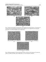
Fig. 12. Neural Network Predictive control response
0 1000 2000 3000 4000 5000
0
500
1000

time, sec
T
D
, °C


Reference
Ac tual
T
D
0 1000 2000 3000 4000 5000
-5
0
5
time, sec
e
, °C

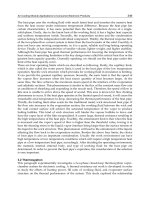
Fig. 13. Piecewise Linearized Model Predictive control response
4.5 Discrete controller tuning online
Control loop of this technique is connected in a way introduced briefly in section 3.3.
Differential evolution is chosen as search technique. After some experiments, eligible
parameters are chosen this way:
NP = 30; CR = 0.85; F = 0.6; N = 20. Cost function is selected
according to Eq. (19), where
h
1
= 0.1, h
2
= 0.01. Control response is depicted in Fig. 14.

There is no exact alternative in classical control theory to this technique. However, in a
certain way it is close to predictive control, therefore it can be compared to Fig. 13.
It is remarkable, that control response shown in Fig. 14 provides the most suitable
performance of all experiments. But, on the other hand, it is highly computationally
demanding technique.
Artificial Neural Network – Possible Approach to Nonlinear System Control

375
0 1000 2000 3000 4000 5000
0
500
1000
time, sec
T
D
, °C


Reference
Ac tual
T
D
0 1000 2000 3000 4000 5000
-1
0
1
2
time, sec
e
, °C

Fig. 14. Discrete controller tuned online
5. Conclusion
The aim of this work was to design a controller, which provides control performance with
control error less than 10°C. Because of the nonlinearity of the plant, two groups of
advanced control techniques were used. The first group is based on artificial neural
networks usage while the second one combines their alternatives in modern control theory.
Generally speaking, neural networks are recommended to use when plant is strongly
nonlinear and/or stochastic. Although reactor furnace is indispensably nonlinear, it is
evident that control techniques without neural networks can control the plant sufficiently
and in some cases (especially predictive control and internal model control) even better.
Thus, neural network usage is not strictly necessary here, although especially Discrete
Controller Tuning Online brings extra good performance.
6. Acknowledgement
This work was supported by the 6th Framework Programme of the European Community
under contract No. NMP2-CT-2007-026515 "Bioproduction project - Sustainable Microbial
and Biocatalytic Production of Advanced Functional Materials" and by the funds No. MSM
6046137306 and No. MSM 0021627505 of the Czech Ministry of Education. This support is
very gratefully acknowledged.
7. References
Baotic, M.; Christophensen, F.; Morari , M. (2006). Constrained Optimal Control of Hybrid
Systems With a Linear Performance Index.
IEEETrans. on Automatic Control, Vol.51,
No 12., ISSN 1903-1919.
Camacho, E.F.; Bordons, C. (2007).
Model Predictive Control, Springer-Verlag, ISBN 1-85233-
694-3, London
Artificial Neural Networks - Industrial and Control Engineering Applications

376

Coello, C. A. C.; Lamont, G. B. (2002). Evolutionary Algorithms for Solving Multi-Objective
problems
, Springer, ISBN 978-0-387-33254-3, Boston
Dolezel, P.; Taufer, I. (2009a). PSD controller tuning using artificial intelligence techniques,
Proceedings of the 17th International Conference on Process Control ’09, pp. 120-124,
ISBN 978-80-227-3081-5, Strbske Pleso, june 2009, STU, Bratislava.
Dolezel, P.; Mares, J. (2009b). Reactor Furnace Control using Artificial Neural Networks and
Genetic Algoritm,
Proceedings of the International Conference on Applied Electronics,
pp. 99-102, ISBN 978-80-7043-781-0, Plzen, september 2009, ZCU, Plzen.
Dwarapudi, S.; Gupta, P. K.; Rao, S. M. (2007). Prediction of iron ore pellet strength using
artificial neural network model,
ISIJ International, Vol. 47, No 1., ISSN 0915-1559.
Economou, C.; Morari, M.; Palsson, B. (1986). Internal Model Control: extension to nonlinear
system,
Industrial & Engineering Chemistry Process Design and Development, Vol. 26,
No 1, pp. 403-411, ISSN 0196-4305.
Fletcher, R. (1987).
Practical Methods of Optimization, Wiley, ISBN 978-0-471-91547-8,
Chichester, UK.
Lichota, J. ; Grabovski, M. (2010). Application of artificial neural network to boiler and
turbine control,
Rynek Energii, ISSN 1425-5960.
Mares, J., Dusek, F., Dolezel, P.(2010a) Nelinearni a linearizovany model reaktorové pece. In
Proceedings of Conference ARTEP’10", 24 26. 2 2010.Technicka univerzita Kosice,
2010. Pp. 27-1 – 27-14. ISBN 978-80-553-0347-5.
Mares, J., Dusek, F., Dolezel, P.(2010b). Prediktivni rizeni reaktorove pece.
In Proceedings of
XXXVth Seminary ASR’10 „Instruments and Control"
, VSB- Technical University

Ostrava, 2010. Pp. 269 – 279.
ISBN 978-80-248-2191-7.
Montague, G.; Morris, J. (1994). Neural network contributions in biotechnology, Trends in
biotechnology,
Vol. 12, No 8., ISSN 0167-7799.
Nguyen, H.; Prasad, N.; Walker, C. (2003).
A First Course in Fuzzy and Neural Control,
Chapman & Hall/CRC, ISBN 1-58488-244-1, Boca Raton.
Norgaard, M.; Ravn, O.; Poulsen, N. (2000).
A Neural Networks for Modelling and Control of
Dynamic Systems
, Springer-Verlag, ISBN 978-1-85233-227-3, London.
Rivera, D.; Morari, M.; Skogestad, S. (1986). Internal Model Control: PID Controller Design,
Industrial & Engineering Chemistry Process Design and Development, Vol. 25, No 1., pp.
252-265, ISSN 0196-4305.
Teixeira, A.; Alves, C.; Alves, P. M. (2005). Hybrid metabolic flux analysis/artificial neural
network modelling of bioprocesses,
Proceedings of the 5th International Conference on
Hybrid Intelligent Systems
, ISBN 0-7695-2457-5, Rio de Janeiro.
18
Direct Neural Network Control via Inverse
Modelling: Application on Induction Motors
Haider A. F. Almurib
1
, Ahmad A. Mat Isa
2
and Hayder M.A.A. Al-Assadi
2

1
Department of Electrical & Electronic Engineering, The University of Nottingham
Malaysia Campus Semenyih, 43500
2
Faculty of Mechanical Engineering, University Technology MARA (UiTM)
Shah Alam, 40450
Malaysia

1. Introduction
Applications of Artificial Neural Networks (ANNs) attract the attention of many scientists
from all over the world. They have many advantages over traditional algorithmic methods.
Some of these advantages are, but not limited to; ease of training and generalization,
simplicity of their architecture, possibility of approximating nonlinear functions,
insensitivity to the distortion of the network and inexact input data (Wlas et al., 2005). As for
their applications to Induction Motors (IMs), several research articles have been published
on system identification (Karanayil et al., 2003; Ma & Na, 2000; Toqeer & Bayindir, 2000;
Sjöberg et al. 1995; Yabuta & Yamada, 1991), on control (Kulawski & Brys, 2000; Kung et al.,
1995; Henneberger & Otto, 1995), on breakdown detection (Raison, 2000), and on estimation
of their state variables (Simoes & Bose, 1995; Orłowska-Kowalska & Kowalski, 1996).
The strong identification capabilities of artificial neural networks can be extended and
utilized to design simple yet good performance nonlinear controllers. This chapter
contemplates this property of ANNs and illustrates the identification and control design
processes in general and then for a given system as a case study.
To demonstrate its capabilities and performance, induction motors which are highly
nonlinear systems are considered here. The induction machine, especially the squirrel-cage
induction motor, enjoys several inherent advantages like simplicity, ruggedness, efficiency
and low cost, reliability and compactness that makes it the preferred choice of the industry
(Vas, 1990; Mehrotra et al., 1996; Wishart & Harley, 1995; Merabet et al., 2006; Sharma, 2007).
On the other hand, advances in power switching devices and digital signal processors have
significantly matured voltage-source inverters (VSIs) with the associated pulse width

modulation (PWM) techniques to drive these machines (Ebrahim at el., 2010). However, IMs
comprise a theoretically challenging problem in control, since they are nonlinear
multivariable time-varying systems, highly coupled, nonlinear dynamic plants, and in
addition, many of their parameters vary with time and operating condition (Mehrotra et al.,
1996a; 1996b; Merabet et al., 2006).
Artificial Neural Networks - Industrial and Control Engineering Applications

378
2. System identification
This chapter will carry out the system identification of an induction motor using the
artificial neural network and precisely the Back Propagation Algorithm. The procedure used
to identify the system is as described in Fig.1.

Data Collection
(Experimental Work)
Selecting the Model
Structure
Fitting the Model
to the Data
Validating the Model
Accepting the Model ?
Yes
No
Model structure is not good
Data is not good
Insert Filtration
Factor
if Necessary

Fig. 1. System identification loop

Now, the system identification problem would be as follows: We have observed inputs, u(t),
and outputs, y(t), from the plant under consideration (induction motor):

(
)
(
)
(
)
1, 2, ,
t
uuu ut
=⎡ ⎤
⎣
⎦
"
(1)

(
)
(
)
(
)
1, 2, ,
t
y
yy yt
=⎡ ⎤
⎣

⎦
"
(2)
where
t
u is the input signal to the plant (input to the frequency inverter) and
t
y
is the
output signal (measured by the tacho-meter representing the motor’s speed). We are looking
for a relationship between past
11
,
tt
uy
−−
⎡
⎤
⎣
⎦
and future output, y(t):

(
)
(
)
ˆ
|,
y
tgt

θ
ϕθ
=⎡ ⎤
⎣⎦
(3)
where
ˆ
y
denotes the model output which approximates the actual output
()
y
t ,
g
is a
nonlinear mapping that represents the model,
(
)
t
ϕ
is the regression vector given by

()
(
)
11
,
tt
tuy
ϕϕ
−−

= (4)
Direct Neural Network Control via Inverse Modelling: Application on Induction Motors

379
and its components are referred to as regressors. Here,
θ
is a finite dimensional parameter
vector, which is the weights of the network in our case (Bavarian, 1988; Ljung & Sjöberg,
1992; Sjöberg et al. 1995).
The objective in model fitting is to construct a suitable identification model (Fig. 2) which
when subjected to the same input
(
)
ut to the plant, produces an output
()
ˆ
y
t which
approximates
()
y
t . However, in practice, it is not possible to obtain a perfect model. The
solution then is to select
θ
in Eq. (3) so as to make the calculated values of
(
)
ˆ
|
yt

θ
fit to the
measured outputs
(
)
y
t as close as possible. The fit criterion will be based on the least
square method given by

(
)
min ,
N
Vt
θ
θϕ
⎡
⎤
⎣
⎦
(5)
where

() () ( )
2
1
1
ˆ
,|
N

N
t
Vt ytyt
N
θϕ θ
=
⎡
⎤= ⎡ − ⎤
⎣
⎦⎣ ⎦
∑
(6)
Hence, the error
ε
is given by

(
)
(
)
(
)
ˆ
|
tytyt
ε
θ
=− (7)
This is illustrated in Fig. 2.

+
-
Plant
Plant
P
M
()
ty
()
ty
ˆ
()
t
ε
()
tu

Fig. 2. Forward plant modelling
3. Artificial Neural Networks
Strong non-linearities and model uncertainty still pose a major problem for control
engineering. Adaptive control techniques can provide solutions in some situations however
in the presence of strongly non-linear behaviour of the system traditional adaptive control
algorithms do not yield satisfactory performance. Their inherent limitations lie in the
linearization based approach. A linear model being a good approximation of the non-linear
plant for a given operation point cannot catch up with a fast change of the state of the plant
and poor performance is observed until new local linear approximation is built.
Artificial neural networks offer the advantage of performance improvement through
learning using parallel and distributed processing. These networks are implemented using
massive connections among processing units with variable strengths, and they are attractive
for applications in system identification and control.

Artificial Neural Networks - Industrial and Control Engineering Applications

380
3.1 The network architecture
Figure 3 shows a typical two-layer artificial neural network. It consists of two layers of
simple processing units (termed neurons).
The outputs computed by unit j of the hidden-layer and unit k of the output-layer are given
by:

(
)
1, 2, ,
jhj
xfH j h==
(8)

(
)
1, 2, ,
kok
yf
Ik m==
(9)
respectively, where
h
f
and
o
f
are the bounded and differentiable activation functions.

Thus, the output unit k will result in the following:

kkjjii
ji
yf wf vu
⎡
⎤
⎛⎞
=
⎢
⎥
⎜⎟
⎝⎠
⎢
⎥
⎣
⎦
∑∑
(10)
where
k
y here is the vector representing the network output.
It has been formally shown (Lippman, 1987; Fukuda & Shibata, 1992) that Artificial Neural
Networks with at least one hidden layer with a sufficient number of neurons are able to
approximate a wide class continuous non-linear functions to within an arbitrarily small
error margin.

Hidden
layer
j

Input
layer
i
Output
layer
k
v
ji
w
kj
∑ ∑
Hidden unit’s neuron Output unit’s neuron
Biase Biase
i
u
k
y
j
x
k
y

Fig. 3. A two layer artificial neural network
3.2 The training agorithm
In developing a training algorithm for this network, we want a method that specifies how to
reduce the total system error for all patterns through an adjustment of the weights. This
chapter uses the Back-Propagation training algorithm which is an iterative gradient algorithm
designed to minimize the mean square error between the actual output of a feed-forward
network and the desired output (Lippman, 1987; Weber et al., 1991; Fukuda & Shibata, 1992).
Direct Neural Network Control via Inverse Modelling: Application on Induction Motors

381
The back-propagation training is carried out as follows: the hidden layer weights are
adjusted using the errors from the subsequent layer. Thus, the errors computed at the
output layer are used to adjust the weights between the last hidden layer and the output
layer. Likewise, an error value computed from the last hidden layer output is used to adjust
the weights in the next to the last hidden layer and so on until the weight connections to the
first hidden layer are adjusted. In this way, errors are propagated backwards layer by layer
with corrections being made to the corresponding layer weights in an iterative manner. The
process is repeated a number of times for each pattern in the training set until the criterion
minimization is reached. This is illustrated in Fig. 4. Therefore, we first calculate the
predicted error at each time step s (we refer to s here to introduce the discrete time factor).
Then, an equivalent error is calculated for each neuron in the network. For example the
equivalent error
δ
k
of the neuron k in the output layer is given by (taking into account that
the derivative of the output layer’s activation function is unity because it is a linear
activation function):

(
)
(
)
(
)
(
)
ˆ
kkkk

ss
y
s
y
s
δε
==− (11)
The equivalent error
δ
j
of neuron j in the hidden layer is given by:

()
()
(
)
()
()
j
j
kk
j
k
j
df H s
ssw
dH s
δδ
=
∑

(12)
Weights connecting the hidden and output layers are adjusted according to:

(
)
(
)
(
)
() () () ( )
1
1
kj kj kj
kj k j kj
ws ws ws
ws sxs ws
αδ β
=−+Δ
Δ
=+Δ−
(13)
where:
α
and
β
are the learning rate and the momentum parameters respectively.
Weights connecting the input and hidden layer are adjusted according to:

(
)

(
)
(
)
() () () ( )
1
1
ji ji ji
ji j i ji
vs vs vs
vs sus vs
αδ β
=−+Δ
Δ
=+Δ−
(14)

y
d
u
v
ji
w
kj
k
i
j
δ
δ
∑

Desired
Output
Network
Output

Fig. 4. Back-propagation algorithm
In summary, the training algorithm is as follow: the output layer error is calculated first
using Eq. (11) and then backpropagated through the network using Eq. (12) to calculate the
Artificial Neural Networks - Industrial and Control Engineering Applications

382
equivalent errors of the hidden neurons. The network weights are then adjusted using
Eq. (13) and Eq. (14).
3.3 Model validation
In order to check if the identified model agrees with the real process behavior, model
validation is necessary. This is imperative as to taken into account the limitations of any
identification method and its final goal of model application. This includes a check to
determine if the priori assumptions of the identification method used are true and to
compare the input-output behaviour of the model and the plant (Ljung & Guo, 1997).
To validate the model, a new input will be applied to the model under validation tests. The
new outputs will be compared with the real time outputs and validation statistics is
calculated. These statistics will decide whether the model is valid or not.
To carry out the validation task, we use the following statistics for the model residuals:
The maximal absolute value of the residuals

(
)
1
max
NtN

M
t
ε
ε
≤≤
= (15)
Mean, Variance and Mean Square of the residuals

()
1
1
N
N
t
mt
N
ε
ε
=
=
∑
(16)

()
2
1
1
N
NN
t

Vtm
N
εε
ε
=
⎡
⎤
=−
⎣
⎦
∑
(17)

()
()
2
2
1
1
N
NNN
t
StmV
N
ε
εε
ε
=
==+
∑

(18)
In particular we stress that the model errors must be separated from any disturbances that
can occur in the modelling. As this can correlates the model residuals and the past inputs.
This plays a crucial role. Thus, it is very useful to consider two sources of model residuals or
model errors
ε
. The first error originates from the input
(
)
ut while the other one originates
from the identified model itself. If these two sources of error are additive and the one that
originates from the input is linear, we can write

(
)
(
)
(
)
(
)
t
q
ut vt
ε
=Δ + (19)
Equation (19) is referred to as the separation of the model residuals and the disturbances.
Here,
v(t) would not change, if we changed the input u(t). To check the part of the residuals
that might originate from the input, the following statistics are frequently used:

If past inputs are
(
)
(
)
(
)
(
)
,1,, 1
T
tutut utM
φ
=
⎡− −+⎤
⎣
⎦
"
and
() ()
1
1
N
T
N
t
Rtt
N
φφ
=

=
∑
, then the
scalar measure of the correlation between past inputs
(
)
t
φ
and the residuals
(
)
t
ε
is given by:

1MT
NuNu
rRr
ε
ε
ξ
−
= (20)
Direct Neural Network Control via Inverse Modelling: Application on Induction Motors

383
where
() ( )
0, , 1
T

uu u
rr rM
εε ε
=⎡ − ⎤
⎣⎦
"
with
() () ( )
1
1
N
u
t
rtut
N
ε
τ
ετ
=
=−
∑
.
The obtained model should pass the validation tests of a given data set. Then we can say
that our model is unfalsified. Here, we shall examine our model when the validation test is
based on some of the statistics given previously in Eqs. (15-20).
Let us first assume that the model validation criterion be a positive constant
0
μ
> for the
maximal absolute value of the residuals

N
M
ε
stated in Eq. (15)

(
)
(
)
, is not validated iff
N
gt M
ε
ϕ
θθμ
⎡
⎤≤
⎣⎦
(21)
The problem of determining which models satisfy the inequality of Eq. (21) is the same
problem that deals with set membership identification (Ninness & Goodwin, 1994).
Typically this set is quite complicated and it is customary to outerbound it either by an
ellipsoid or a hypercube. Therefore, it is agreed that a reasonable candidate model for the
true dynamics should make the sample correlation between residuals
(
)
(
)
(
)

ˆ
,|
tytyt
ε
θθ
=−
and past inputs
(
)
(
)
1, ,ut ut m−−" small within certain criterion. One possible validation
criterion is to require this correlation to be small in comparison with the Mean Square of the
Model Residuals
N
S
ε
stated in Eq. (18). This is given by:

(
)
(
)
(
)
, is not validated iff
M
NN
gt S
ε

ϕ
θξθγθ
⎡⎤ ≤
⎣⎦
(22)
where
γ
is a subjective threshold that will be selected according to the application.
4. The neurocontroller
Conceptually, the most fundamental neural network based controllers are probably those
using the inverse of the plant as the controller. The simplest concept is called direct inverse
control, which is used in this chapter. Before considering the actual control system, an
inverse model must be trained. There are tow ways of training the model; generalized
training and the specialized training. This chapter uses the generalized training method.
Figure 5 shows the off-line diagram of the inverse plant modelling.

Plant
Plant
P
C
(
)
ε
t
(
)
yt
(
)


ut
(
)
ut
(
)
rt

Fig. 5. Inverse plant modelling
Given the input-output data set which will be referred to as
N
Z over the period of time
1 tN≤≤

(
)
(
)
(
)
(
)
{
}
1, 1, , ,
N
Zuy uNyN= (23)
Artificial Neural Networks - Industrial and Control Engineering Applications

384

where u(t) is the input signal and
(
)
y
t is the output signal, the system identification task is
basically to obtain the model
(
)
θ
|
ˆ
ty that represent our plant;

()
(
)
ˆ
|,
N
y
tgZ
θθ
= (24)
where
ˆ
y denotes the model output and
g
is some non-linear function parameterized by
θ

which is the finite dimensional parameter vector, the weights of the network in our case
(Ljung & Sjöberg 1992; Ljung, 1995; Sjöberg, 1995).
The objective with inverse plant modelling is to formulate a controller, such that the overall
controller-plant architecture has a unity transfer function, i.e., if the plant can be described
as in Eq. (24), a network is trained as the inverse of the process:

()
(
)
1
ˆ
|,
N
ut g Z
θθ
−
= (25)
However, modelling errors perturb the transfer function away from unity. Therefore,
(
)
1
ˆ
,
N
gZ
θ
−
will be used instead of
(
)

1
,
N
gZ
θ
−
.
To obtain the inverse model in the generalized training method, a network is trained off-line
to minimize the following criterion instead:

()
() ( )
()
2
1
1
ˆ
,|
N
N
N
t
WZ utut
N
θθ
=
=−
∑
(26)
In other words, our aim is to reduce the error

ε
where:

(
)
(
)
(
)
ˆ
|tutut
ε
θ
=−
(27)
Once we carry out that, the inverse model is subsequently applied as the controller for the
system by inserting the desired output (the reference) instead of the system output. This is
illustrated in Fig. 6.

()
yt
+
1
()
ut
Plant
DD
D
()
rt

+
1
Inverse Model
Controller

Fig. 6. Direct inverse control
5. Simulation and results
The first step is to collect training data from the real plant, which is a three phase squirrel-
cage induction motor with the following ratings: 380V, 50Hz, 4-pole, 0.1kW, 1390rpm, and is
Direct Neural Network Control via Inverse Modelling: Application on Induction Motors

385
Y-connected. That was carried out by using a data acquisition card to interface the induction
motor and the inverter and its inputs and outputs to the computer. A voltage signal is to be
sent to the frequency inverter which changes the three phase lines frequency into a new
signal with different frequency to drive the induction machine speed. That was the input
signal. The output signal is taken from a tachometer connected directly to the rotor shaft
and back to the interfacing data acquisition card as the speed signal. Figure 7 shows the
overall experimental system setup.

Frequency
Inverter
Interfacing Data
Aquisition Card
Tachometer
Induction
Motor
Computer
Motor

Fig. 7. The experimental work
5.1 Results of system identification
The input data set is designed to be a PRBS signal chosen randomly, both in amplitude and
frequency, to fully excite the whole speed range which allows the network to recognize the
overall system’s behaviour. In addition, the sampling time is made to be 40 times smaller
than the settling time of the system to obtain more accurate model and avoid aliasing
problems. The input-output data set is shown in Fig. 8. The data set will be divided into two
sets; a network training set and a model validation set.

0 1000 2000 3000 4000 5000 6000
0
500
1000
1500
2000
Samples
Output Signal
0 1000 2000 3000 4000 5000 6000
0
500
1000
1500
In p u t S i g n a l
The Input-Output Da ta S e t.
Input-Output Data Set
Input Signal
Output Signal
Sam
p
les

Fig. 8. The input-output data set
Artificial Neural Networks - Industrial and Control Engineering Applications

386
Since the system is a single-input single-output nonlinear system, this work uses a second
order NARX model. This means that the regressor vector is as follows:

() ()()()()
1, 2, 1, 2tyt yt ut ut
ϕ
=
⎡− − − −⎤
⎣
⎦
(28)
The network structure is a two-layer hyperbolic tangent sigmoidal feed-forward
architecture (one hidden layer with a tanh activation function and one output layer with a
linear activation function). The weights for both hidden layer and output layers are initially
randomized around the values of -0.5 and +0.5 before the training. This is useful so that the
training would fall in a global minima rather than a local minima (Patterson, 1996).
Too many hidden neurons can cause the over-fitting, while too few neurons cause the
under-fitting (Patterson, 1996). Moreover, a big network (many neurons) causes the training
process to become very slow. The training showed good results when a five hidden neurons
is used and 3000 samples are used as a training set. During each back propagation iteration
the Sum of Squared Errors (SSE) are computed and compared to an error criteria
α
, i.e.

() ()

2
1
ˆ
N
i
SSE y t y t
α
=
=
⎡−⎤<
⎣⎦
∑
(29)

The SSE decreased gradually during the training process until it is within the criteria
threshold after approximately 370 iterations. To test whether the network can produce the
same output as the plant or not, and considering the over-fitting problem, the output
(
)
ˆ
|yt
θ
of the model will be compared with the plant output
(
)
y
t to calculate the residuals
(
)
(

)
(
)
ˆ
|tytyt
ε
θ
=− . The results of applying both training and validation data sets are
shown in Table 1.


0 2 4 6 8 10 12 14 16 18 20
0
1000
2000
SSE [1:20]
The S um S q uare d Error During the Training P roce s s
0 20 40 60 80 100 120 140 160
0
5
10
SSE [21:180]
0 20 40 60 80 100 120 140 160 180 200
1
1.02
1.04
Iterations
SSE [181:370]

Fig. 9. The Sum Squared Error during the training process
Direct Neural Network Control via Inverse Modelling: Application on Induction Motors

387
Residual Statistics Training data set Validation data set
Mean Square
N
S
ε

4
2.869 10
−
⋅
4
2.936 10
−
⋅
Maximal Absolute Value
N
M
ε

2.9692% 3.0286%
Table 1. Residual Analysis
From the table we can see that there are only small differences in the residual statistics
between the training data set and the validation data set. Thus the inequality of Eq. (21) is
satisfied. However, one should check the correlation
M
N

ξ
between the residuals
(
)
,t
ε
θ
and
past inputs
()
(
)
1, ,ut ut m−−" because the residual statistics are not enough to judge the
quality of the network model. This is done by constructing the past input vector and then
calculating the correlation function.
The correlation results are shown in Fig. 9, where it can be seen that the auto-correlation of
the residuals lies within the 99% confidence limits which gives a strong indication that the
model is acceptable. Furthermore, we can see that the cross correlation between the past
inputs and the residuals lies between the 99% confidence limits also.

0 5 10 15 20 25
-0.5
0
0.5
1
La g
Auto Corre la tio n Functio n of the Re s idua ls
-25 -20 -15 -10 -5 0 5 10 15 20 25
-0.1
0

0.1
La g
C ros s C orre la tion Be twe e n the Re s idua ls a nd the P a s t Inputs
Auto Correlation Function of the Residuals
Cross Correlation between the Residuals and Past Inputs
Lag
La
g

Fig. 9. Correlation Analysis of the Validation Data Set
5.2 Results of inverse training and control
As mentioned earlier, it is clear that the plant is a single-input single-output (SISO) system.
First the regressors are chosen based on inspiration from linear system identification. The
model order was chosen as a second order which gave us good results. Clearly, the input
vector to the network contains two past plant outputs and two past plant inputs.

(
)
(
)
(
)
(
)
1, 2, 1, 2
N
Zytyt utut
=
⎡− − − −⎤
⎣

⎦
(30)
The network structure is a two layer hyperbolic tangent sigmoidal feed-forward architecture
(one hidden layer with a tanh activation function and one output layer with a linear
Artificial Neural Networks - Industrial and Control Engineering Applications

388
activation function). The network weights are initially randomised around the values -0.5
and +0.5 before the training.
The back-propagation training showed good results when using a network structure with
two layer feed forward architecture neuron and 3000 samples as a training set. The network
architecture contains one hidden layer with a hyperbolic tangent (tanh) activation function
and one output layer with a linear activation function. The hidden layer consists of six
hidden neurons while the output layer consists of one neuron. The results of the inverse
plant model training algorithm is shown in Fig. 10 where
α
is chosen as 1.

0 5 10 15 20 25 30 35 40 45 50
0
100
200
300
400
500
SSE (1:50)
The S um S qua re d Error During The Tra ining P roce ss .
0 50 100 150 200 250 300 350 400 450
1
1.02

1.04
1.06
SSE (51:488)
It e r a t i o n s
Sum Squared Errors During Training Process
SSE (1:50)
SSE (51:488)
Iterations

Fig. 10. SSE of inverse plant modelling

0 1 2 3 4 5 6 7 8 9 10
0
200
400
600
800
1000
1200
1400
1600
1800
Time [seconds]
Speed [rpm]
Unit Step Re s pons e with Direct Inverse Control.

Fig. 11. Speed error due to a step reference signal
Direct Neural Network Control via Inverse Modelling: Application on Induction Motors

389

The final step after obtaining the inverse model is to implement the controller. The same
setup of Fig. 7 is used to control the speed of the motor. First, to check the controller
performance, a step input signal with the value of 1390rpm is fed to the system. The
resulting response and error between the reference signal and the measured output speed

0 0.5 1 1.5 2 2.5 3 3.5 4 4.5 5
-500
0
500
1000
1500
S pe ed E rro r [0:5 se conds ]
S pe ed E rror with Dire ct Inve rse Control.
5 5.5 6 6.5 7 7.5 8 8.5 9 9.5 10
-5
0
5
Time [seconds]
Speed Error [5:10 seconds]
Speed Error with Direct Inverse Control
Speed Error [0:5 sec]
Time [sec]
Speed Error [5:10 sec]

Fig. 12. Speed error due to a step reference signal

0 2 4 6 8 10 12 14 16
0
200
400

600
800
1000
1200
1400
1600
1800
Time [seconds]
Speed [rpm]
S qua re Wa ve Re fe re nc e a nd S p ee d Re sponse of Dire ct Inve rs e C ontrol S che me .
Speed Response to Square-wave Reference Signal
Speed [rpm]
Time
[
sec
]

Fig. 13. System response to a square wave reference signal
Artificial Neural Networks - Industrial and Control Engineering Applications

390
are illustrated in Figs. 11 and 12 respectively. It can be seen from Fig. 12 that the speed of the
induction motor followed the reference signal with an acceptable steady state error equals to
0.2878%. The results of Figs. 11 and 12 also show a maximum overshoot of less than 13%.
To investigate the tracking capabilities of the system, different reference signals were fed to
the controller and its performance is examined. The following real time tests will explore

0 2 4 6 8 10 12 14 16
0
500

1000
1500
Time [seconds]
Speed [rpm]
Sine Wave Reference and Speed Response of Direct Inverse Control Scheme.
Speed Response to Sine-wave Reference Signal
Speed [rpm]
Time
[
sec
]

Fig. 14. System response to a sine wave reference signal

0 2 4 6 8 10 12 14 16
0
200
400
600
800
1000
1200
1400
1600
Time [s e co nds ]
Speed [rpm]
Ramp Wave Reference and Speed Response of Direct Inverse Control Scheme.
Speed Response to Ramp-wave Reference Signal
Speed [rpm]
Time

[
sec
]

Fig. 15. System response to a saw-tooth wave reference signal
Direct Neural Network Control via Inverse Modelling: Application on Induction Motors

391
the response to three different types of speed reference signals; square wave (Fig. 13), sine
wave (Fig. 14), and saw-tooth wave (Fig. 15) reference signals. In addition, the steady state
errors are recorded in Table 2.


Reference Signal Min. Error Max. Error
Square wave
0.31%− 0.56%
+

Sine wave
0.43%− 1.00%
+

Saw-tooth wave
0.65%− 0.29%
+

Table 2. Steady state errors analysis for different reference signal types

The previous figures suggest that the direct inverse model control scheme can track changes
in the reference signal while maintaining good performance.

Next, to test the system under disturbances in the form of load torque conditions, a step
reference signal representing 1390 rpm is fed to the system while a load torque step signal of
2 N.m (which is the full load) is applied to the shaft during the period of 4 to 8 seconds. The
results are shown in Fig. 16. It can be seen from the figure that the direct inverse controller
could recover the disturbance caused by the applied load torque. The induction motor speed
followed the reference signal in a short time.


0 2 4 6 8 10 12
0
200
400
600
800
1000
1200
1400
1600
Time [seconds]
Speed [rpm]
Speed Response when Applying a Load Signal Under Direct Inverse Control Scheme.
Speed Response under Applied Load Torque
Speed [rpm]
Time
[
sec
]

Fig. 16. Speed response under load torque condition
Artificial Neural Networks - Industrial and Control Engineering Applications

392
6. Conclusion
In this chapter, the nonlinear black box modelling for an induction motor is carried out
using the back propagation training algorithm. Half of the experimentally collected data
was employed for ANN training and the other half was used for model validation.
Applying the validation tests, the network model could pass the residual tests and the cross
correlation tests resulting into a simple yet a highly accurate model of the induction motor.
The same method was then used to model the inverse model of the system. The real time
implementation for the direct inverse neural network based control scheme has been
presented and its performance has been tested over different types of reference signals and
applied load torque. The controller tracked the given reference speed signals and overcame
the applied load torque disturbance demonstrating the strong capabilities of artificial neural
networks in nonlinear control applications.
7. References
Bavarian B. (1988). Introduction to Neural Networks for Intelligent Control, IEEE Control
Systems Magazine, Vol. 8, No. 2, pp. 3-7.
Ebrahim Osama S., Mohamed A. Badr, Ali S. Elgendy, and Praveen K. Jain,(2010). ANN-
Based Optimal Energy Control of Induction Motor Drive in Pumping Applications.
IEEE Transactions On Energy Conversion, Vol. 25, No. 3, (Sept. 2010), pp. 652-660.
Fukuda T. & Shibata T. (1992). Theory and Application of Neural Networks for Industrial
Control Systems, IEEE Trans. on Industrial Electronics, Vol. 39, No. 6, pp. 472-489.
Henneberger G. and B. Otto (1995). Neural network application to the control of electrical
drives. Proceeding of Confrence of Power Electronics Intelligent Motion, pp. 103–123,
Nuremberg, Germany.
Karanayil B.; Rahman M. F. & Grantham C. (2003). Implementation of an on-line resistance
estimation using artificial neural networks for vector controlled induction motor
drive, Proceeding of IECON '03 29th Annual Conference of the IEEE Industrial
Electronics Society, Vol. 2, pp. 1703-1708.
Kulawski G. and Mietek A. Brdyś (2000). Stable adaptive control with recurrent networks.

Automatica A Journal of IFAC, the International Federation of Automatic Control, vol. 36,
No. 1, (Jan. 2000), pp. 5–22.
Kung Y. S., C. M. Liaw, and M. S. Ouyang (1995). Adaptive speed control for induction
motor drive using neural network. IEEE Transactions on Industrial Electronics, vol.
42, no. 1, (Feb. 1995), pp. 9–16.
Lippman R. P. (1987). An Introduction to Computing with Neural Nets, IEEE ASSP
Magazine, Vol. 4, pp. 4-22.
Ljung L. & Guo L. (1997). Classical model validation for control design purposes,
Mathematical Modelling of Systems, 3, 27–42.
Ljung L. & Sjöberg J. (1992). A System Identification Perspective on Neural Nets, Technical
Report, Report No. LiTH-ISY-R-1373, At the location: www.control.isy.liu.se, May 27.
Ljung L. (1995). System Identification, Technical Report, Report No. LiTH-ISY-R-1763, At the
location: www.control.isy.liu.se.
Direct Neural Network Control via Inverse Modelling: Application on Induction Motors

393
Ma X. & Na Z. (2000). Neural network speed identification scheme for speed sensor-less
DTC induction motor drive system, PIEMC 2000 Proceeding. 3rd Int. Conference on
Power Electronics and Motion Control, Vol. 3, pp. 1242-1245.
Mehrotra P. ; Quaicoe J. E. & Venkatesan R. (1996a). Development of an Artificial Neural
Network Based Induction Motor Speed Estimator, PESC '96 IEEE Power Electronics
Specialists Conference, Vol. 1, pp. 682-688.
Mehrotra P.; Quaicoe J. E. & Venkatesan R. (1996b). Induction Motor Speed Estimation
Using Artificial Neural Networks, IEEE Canadian Conference on Electrical and
Computer Engineering, Vol. 2, pp. 607-610,
Merabet Adel, Mohand Ouhrouche and Rung-Tien Bui (2006). Neural Generalized
Predictive Controller for Induction Motor, International Journal of Theoretical and
Applied Computer Sciences, Vol. 1, 1 (2006), pp. 83–100.
Mohamed H. A. F.; Yaacob S. & Taib M. N. (1997). Induction Motor Identification Using
Artificial Neural Networks, APEC 97 Electric Energy Conference, pp. 217-221, 29-30th

Sep
Ninness B. & Goodwin G. C. (1994). Estimation of Model Quality, 10th IFAC Symposium
Proceeding. on System Identification, 1, pp. 25-44.
Orłowska-Kowalska T. and C. T. Kowalski (1996). Neural network based flux observer for
the induction motor drive. Proceedingceding of International Confrence of Power
Electronics Motion Control, pp. 187–191, Budapest, Hungary, 1996.
Patterson D. W. (1996). Artificial Neural Networks: Theory and Applications, Simon and
Schuster (Asia) Pte. Ltd., Singapore: Prentice Hall.
Raison B., F. Francois, G. Rostaing, and J. Rogon (2000). Induction drive monitoring by
neural networks. Proceeding of IEEE International Conference of Industrial
Electronics,Control Instrumentation, pp. 859–863, Nagoya, Japan, 2000.
Sharma A. K., R. A. Gupta, Laxmi Srivastava (2007). Performance of Ann Based Indirect
Vector Control Induction Motor Drive, Journal of Theoretical and Applied Information
Technology, Vol. 3, No. 3, (2007), pp 50-57.
Simoes M. G. and B. K. Bose (1995).Neural network based estimation of feedback signals for
a vector controlled induction motor drive. IEEE Transactions on Industry
Applications., vol. 31, no. 3, (May/Jun. 1995), pp. 620–629.
Sjöberg J.; Zhang Q., Ljung L., Benveniste A., Deylon B., Glorennec P. Y., Hjalmarsson H., &
Juditsky A. (1995). Nonlinear Black-Box Models In System Identification: A Unified
Overview, Automatica, Vol. 31, No. 12, pp. 1691-1724.
Toqeer R. S. & Bayindir N. S. (2000). Neurocontroller for induction motors, ICM 2000.
Proceeding. 12th Int. Conference on Microelectronics, pp. 227-230.
Vas P. (1990). Vector Control of AC Machines, Clarendon Press, Oxford.
Weber M.; Crilly P. B. & Blass W. E. (1991). Adaptive Noise Filtering Using an Error-
Backpropagation Neural Network, IEEE Trans. Instrum. Meas., Vol. 40(5), pp. 820-825.
Wishart M. T. & Harley R. G. (1995). Identification And Control Of Induction Machines
Using Artificial Neural Networks, IEEE Transactions on Industry Applications, Vol.
31(3), pp. 612-619.
Artificial Neural Networks - Industrial and Control Engineering Applications

394
Wlas M.; Krzeminski, Z.; Guzinski, J.; Abu-Rub, H.; Toliyat, H.A. (2005). Artificial-
Neural-Network-Based Sensorless Nonlinear Control of Induction Motors, IEEE
Transection of Energy conversion, Vol. 20, 3 (Sept 2005), pp. 520-528.
Yabuta T. & Yamada T. (1991). Learning Control Using Neural Networks. Proceeding of the
1991 IEEE International Conference on Robotics and Automation, Vol. 1, pp. 740-745.
19
System Identification of NN-based Model
Reference Control of RUAV during Hover
Bhaskar Prasad Rimal
1
, Idris E. Putro
2
, Agus Budiyono
2
,
Dugki Min
3
and Eunmi Choi
1
1
Graduate School of Business IT, Kookmin University
Jeongneung-Dong, Seongbuk-Gu, Seoul, 136-702, Korea
2
Department of Aerospace Information Engineering, Konkuk University
3
School of Computer Science and Engineering, Konkuk University
Hwayang-dong, Gwangjin-gu, Seoul 13-701,
Korea
1. Introduction

Unmanned aerial vehicles (UAVs) are becoming more and more popular in a wide field of
applications nowadays. UAVs are used in number of military application for gathering
information and military attacks. In the future will likely see unmanned aircraft employed,
offensively, for bombing and ground attack. As a tool for research and rescue, UAVs can
help find humans lost in the wilderness, trapped in collapsed buildings, or drift at sea. It is
also used in civil application in fire station, police observation of crime disturbance and
natural disaster prevention, where the human observer will be risky to fight the fire. There
is wide variety of UAV shapes, sizes, configuration and characteristics. Therefore, there is a
growing demand for UAV control systems, and many projects either commercial or
academic destined to design a UAV autopilot were held recently. A lot of impressive results
had already been achieved, and many UAVs, more or less autonomous, are used by various
organizations.
An Artificial Neural Network (ANN) [3] is an information processing paradigm that is
stimulated by the way biological nervous systems, such as the brain, process information.
The key element of this paradigm is the novel structure of the information processing
system. Basically, a neural network (NN) is composed of a set of nodes (Fig. 1). Each node is
connected to the others via a set of links. Information is transmitted from the input to the
output cells depending of the strength of the links. Usually, neural networks operate in two
phases. The first phase is a learning phase where each of the nodes and links adjust their
strength in order to match with the desired output. A learning algorithm is in charge of this
process. When the learning phase is complete, the NN is ready to recognize the incoming
information and to work as a pattern recognition system.
ANNs, like people, learn by example. An ANN is configured for a specific application, such
as pattern recognition or data classification, through a learning process. Learning in
biological systems involves adjustments to the synaptic connections that exist between the
neurons.
Artificial Neural Networks - Industrial and Control Engineering Applications

396
In recent years, there is a wide momentum of ANNs in the control system arena, to design

the UAVs. Any system in which input is not proportional to output is known as non-linear
systems. The main advantages of ANNs are having the processing ability to model
nonlinear systems. ANNs are very suitable for identification of non-linear dynamic systems.
Multilayer Perceptron model have been used to model a large number of nonlinear plants.
We can vary the number of hidden layers to minimize the mean square error. ANNs has
been used to formulate a variety of control strategies [1] [2]. The NN approach is a good
alternative for physical modeling techniques for nonlinear systems.


Fig. 1. General Neural Network Architecture
A fundamental difficulty of many non-linear control systems, which potentially could
deliver better performance, is extremely difficult to theoretically predict the behavior of a
system under all possible circumstances. In fact, even design envelope of a controller often
remains largely uncertain. Therefore, it becomes a challenging task to verify and validate the
designed controller under all possible flight conditions. A practical solution to this problem
is extensive testing of the system. Possibly the most expensive design items are the control
and navigation systems. Therefore, one of main questions that each system designer has to
face is the selection of appropriate hardware for UAV system. Such hardware should satisfy
the main requirements without contravening their boundaries in terms of quality and cost.
In UAV design this kind of consideration is especially important due to the safety
requirements expressed in airworthiness standards. Therefore question is how to find the
optimal solution. Thus, simulation is necessary. Basically there are two type of simulation is
needed while designing UAVs systems, they are Software-In-the-Loop (SIL) [5] simulation
and Hardware-In-the-Loop (HIL) simulation [4].
To utilize the SIL configuration, the un-compiled software source code, which normally runs
on the onboard computer, is compiled into the simulation tool itself, allowing this software
to be tested on the simulation host computer. This allows the flight software to be tested
without the need to tie-up the flight hardware, and was also used in selection of hardware.
HILS simulates (Fig. 2) a process such that input and output signals show the time-
dependent values as real-time operating components. It is possible to test embedded system

under real time with various test conditions. It provides the UAV developer to test many
aspects of autopilot hardware, finding the real time problems, test the reliability, and many
more.
The simulation can be done with the help of Matlab Simulink program environment. This
program can be considered as a facility fully competent for this task. Simulink is the most

System Identification of NN-based Model Reference Control of RUAV during Hover

397

Fig. 2. UAV Architecture: Hardware-in-the-loop Simulation
popular tool, it was not only used for a SIL Simulation of the complete UAV system but also
to create the simulation code of a HIL Simulator that runs in real time.
The system identification is the first and crucial step for the design of the controller,
simulation of the system and so on. Frequently it is necessary to analyze the flight data in
the frequency domain to identify the UAV system. This paper demonstrates how ANN can
be used for non linear identification and controller design. The simulation processes consists
of designing a simple system, and simulates that system with the help of model reference
control block in Matlab/Simulink [6].
The paper is organized as follows: Section 2 describes some related work. Section 3 deals
with system identification and control on the basis of NNs. Details of design and control
system with NNs approaches is describes in section 4. In section 5, simulations are
performed on RUAVs system and finally, conclusions are drawn in section 6.
2. Related work
Robust control techniques are capable for adapting themselves for changing the dynamics
which are necessary for autonomous flight. This kind of controller can be designed with the
help of system identification.
There are lots of work had already done in UAV area in the context of ANNs. Mettler B. et
al., [12] describe the process and result of the dynamic modeling of a model-scale unmanned
helicopter using system identification. E. D. Beckmann et al., [13] explained the nonlinear

modeling of a small-scale helicopter and the identification of its dynamic parameters using
prediction error minimization methods. NN approaches have excellent performance than
classical technique for modeling and identifying nonlinear dynamic systems [15] [16].
There is also numerous system identification techniques had been developed to model
nonlinear systems. Some of them are Fuzzy identification [20] [27], state-space identification
[21], frequency domain analysis [22], NN based identification [23] [26]. The exception is
given by LPV identification [25] which is applicable for the entire flight envelope. The
learning ability is the beauty of NN that has been utilized widely for system identification
and control applications. Shim D. H. et al. [28] described time-domain system identification
approaches to design the control system for RUAVs.
Artificial Neural Networks - Industrial and Control Engineering Applications

398
3. System identification and control
The main idea of system identification is often to get a model that can be used for controller
design. System identification (SI) [7] provides the idea of making mathematical models of
dynamics systems, starting from experimental data, measurements, and observations.
It is widely used for applications ranging from control system design and signal processing
to time series analysis. The system identification is used to verify and test the control system
parameters that are associated with the six-degree-of-freedom system using the test flight
data. The simulation results and the statistical error analysis are provided for both the cases.
Fig. 5 shows the flow of control system design with the system identification model.
Basically System identification is the experimental approach to process modeling and it
includes the following five steps as shown in Fig. 3
The system considered as a black box (Fig. 4) which receives some inputs that lead to some
output. The concern here is: what kind of parameters for a particular black box can correlate
the observed inputs and outputs?

Experiment Design
Choice of the

Criteria to Fit
Selection of Model Structure
-Linear , Fuzzy Logic, Neural
Network
……………
Parameter Estimation
-Prior Knowledge, Random,
Prior Model
…………
Accepted
Not
Accepted
Model
Validation
Plant Model
Stopping Criteria
Minimum Cost
Errors-In-variables
Early Stopping
……………….
Cost function
-Errors-In-Variables ,
Least Squares , Bayes
……………
Optimization Scheme
-Levenberg-Marquardt,
Gauss-Newton,
Generic Algorithms,
Backpropagation
……………

Fig. 4. System Identification Modeling Procedure