Desalination Trends and Technologies Part 14 docx

Desalination, Trends and Technologies

314

12 3 NS-1 NS
F
msf
W
P
msf
W
R
msf
W
Q
D
es


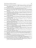
Fig. 3. MFS system
The MSF model considers all the most important aspects of the process.
The heat consumption is calculated by:

F-6b
msf msf
10
Des
QWCpt
ρ
=Δ
(1)

= +
fe
tt tBPE
Δ
ΔΔ+ (2)
Total heat transfer area and number of flash stages are calculated as:

F
max msf
()/
F3
msf msf
10
= ln
f
TtT t
t
e
WCp
t BPE
A
Ut
−
Δ− Δ
⎛⎞
Δ−
⎜⎟
⎜⎟
Δ

⎝⎠
(3)

(
)
F
max msf
f
NS T t T t
=
−Δ − Δ (4)
The total production of distillate is evaluated by:

msf
PF
msf msf
11
NS
f
Cp t
WW
λ
⎡
⎤
Δ
⎛⎞
⎢
⎥
=−−
⎜⎟

⎜⎟
⎢
⎥
⎝⎠
⎣
⎦
(5)
The following equation establishes a relation between heat transfer area, number of tubes
and chamber width:

msf
π
tt
A
TD B N NS=
(6)
The stage height can be approximated by:
2
Hs Lb Ds
=
+ (7)
The number of rows of tubes in the vertical direction is related to the number of tubes in the
following way:

0.481
rt t
NTDN=
(8)
The following equation relates the shell diameter to the number of rows of tubes and Pitch:

2
rt t
Ds N P= (9)
Optimization of Hybrid Desalination Processes
Including Multi Stage Flash and Reverse Osmosis Systems

315
The length of the desaltor is constrained by the following two equations:

P-3
msf
msf
10
d
va
p
va
p
W
L
BV
ρ
= (10)

d
LDsNS=
(11)
The total stage surface area is calculated by:

msf msf

2 2
Sd d
ALB HsLHsBNS
=
++ (12)
Finally, the temperature of last flashing stage of the MSF system is calculated as:

RF
msf max msf

f
TT NStT t
=
−Δ= +Δ (13)
Despite the simplifying hypothesis assumed in the model, the MSF process is well
represented and the solutions of this model are accurately enough to establish conclusions
for the hybrid plant.
3.2 Reverse osmosis model
The model representing the RO system is based on the work (Marcovecchio et al., 2005). A
brief description of the equations is presented here.
Each RO system is composed by permeators operating in parallel mode and under identical
conditions. Particularly, data for DuPont B10 hollow fiber modules were adopted here.
However, the model represents the permeation process for general hollow fiber modules
and any other permeator could be considered providen the particular module parameters.
Figure 4 represents the RO system modeled for the hybrid plant.


Fig. 4. RO system
Initially, pressure of inlet stream is raised by the High Pressure Pumps (HPP). Then, the
pressurized stream passes through membrane modules, where permeation takes place. Part

of the rejected stream could pass through the energy recovery system, before being
discharged back to the sea or fed into the MSF system. Therefore, part of the power required
for the whole plant is supplied by the energy recovery system, and the rest will be provided
by an external source.
Equations (14) to (30) describe the permeation process taking place at one module of each
system.
HPP
ERS
F
ro
W
P
ro
W
R
ro
W
RO Permeators
Desalination, Trends and Technologies

316
The transport phenomena of solute and water through the membrane are modeled by the
Kimura-Sourirajan model (Kimura & Sourirajan, 1967):

(
)
bm P
bp
sss
w

ss
s
6
3600
10 101325
iRT ρ CC
J A PP
Ms
⎛⎞
−
⎜⎟
=−−
⎜⎟
⎜⎟
⎝⎠
s=ro1, ro2 (14)

(
)
mPb
ss
S
s
6
3600
10
BC C
ρ
J
−

= s=ro1, ro2 (15)
The velocity of flow is:

(
)
wS
ss
w
s
p
JJ
V
ρ
+
=
s=ro1, ro2 (16)
The following equation gives the salt concentration of the permeate stream:

S6
P
s
s
p
W
s
10J
C
V
ρ
= s=ro1, ro2 (17)

Permeate flow rate is calculated as the product between the permeation velocity and the
membrane area:

p
w
ssm
QVA= s=ro1, ro2 (18)
The total material balance for each permeator is:

p
fb
sss
QQQ=+ s=ro1, ro2 (19)
The salt balance in each permeator is given by:

p
fF bR P
ss s s ss
QC QC Q C=+ s=ro1, ro2 (20)
The phenomenon of concentration polarization must be considered. The principal negative
consequence of this phenomenon is a reduction in the fresh water flow. The approach
widely used to model the influence of the concentration polarization is the film theory. The
Sherwood, Reynolds and Schmidt numbers are combined in an empirical relation: equation
(24) to calculate the mass transfer coefficient:

s0
s
2k r
Sh
D

=
s=ro1, ro2 (21)

Sb
0s
s
b
2
Re
rU
ρ
μ
= s=ro1, ro2 (22)

b
s
b
μ
Sc
ρ
D
= s=ro1, ro2 (23)
Optimization of Hybrid Desalination Processes
Including Multi Stage Flash and Reverse Osmosis Systems

317

()()
1/3 1/3
sss

2 725 Re Sh . Sc=
s=ro1, ro2 (24)
The concentration polarization phenomenon is modeled by:

mP w
ss s
RP
s
ss
exp
3600
CC V
k
CC
⎛⎞
−
=
⎜⎟
⎜⎟
−
⎝⎠
s=ro1, ro2 (25)
In order to estimate the average pressure drop in the fiber bore and the average pressure
drop on the shell side of the fiber bundle, it is necessary to calculate the superficial velocity
in the radial direction. According to (Al-Bastaki & Abbas, 1999), the superficial velocity can
be approximated as the log mean average of the superficial velocity at the inner and outer
radius of the fiber bundle:

f
si

s
s
i
3600 2 π
Q
U
RL
=
s=ro1, ro2 (26)

fw
so
ssm
s
o
3600 2 π
QVA
U
RL
−
=
s=ro1, ro2 (27)

()
si so
S
ss
s
si so
ss

log
UU
U
UU
−
= s=ro1, ro2 (28)
The approximation for the pressure drop in the fiber bore is based on Hagen-Poiseuille’s
equation:

p
w2
p
os
s
4
i
16
1
1
2
3600 101325
μ
rV L
P
r
=+ s=ro1, ro2 (29)
Similarly, the pressure drop on the shell side of the fiber bundle is estimated by Ergun’s
equation:

()

()
()
(
)
()
2
bS
2
bS
b
s
s
f
s
soi oi
32 3
pp
1.75 1
150 1
11
22
101325 101325
ερ U
εμU
P P RR RR
ε d ε d
−
−
=− − − − s=ro1, ro2 (30)
Finally, the total flow rates of feed and permeate for each system are given by:

Ff
sss
WNMQ= s=ro1, ro2 (31)

p
P
ss
s
WNMQ= s=ro1, ro2 (32)

The chosen model considers all the most important aspects affecting the permeation process.
Even thought, differential equations involved in the modeling are estimated without any
discretization, the whole model is able to predict the flow of fresh water and salt trough the
membrane in an accuracy way.
Desalination, Trends and Technologies

318
3.3 Network equations
The overall superstructure is modelled in such way that all the interconnections between the
three systems are allowed, as it shown in Figure 1.
In effect, part of the rejected stream of each system can enter into another system, even itself.
The fractions of rejected streams of RO systems that will enter into MSF system or that will
be discharged back to the sea, will pass through the ERS. On the contrary, the fractions of
rejected streams of RO systems that will enter into a RO system again, will not pass through
the ERS, because the plant could benefit from these high pressurized streams. In fact, when
all the streams entering to a RO system flow at a high enough pressure, the corresponding
HPPs can be avoided. That RO system would correspond to a second stage of reverse
osmosis. In that case, the pressure of all the inlet streams will be levelled to the lowest one,
by using appropriated valves. However, if at least one of the RO inlet streams is coming

from MSF system or from sea, the pressure of all the inlet streams will be lowered to
atmospheric pressure, and before entering membrane modules, HPPs will be required. The
network and cost equations are formulated is such way that the optimization procedure can
decide the existence or not of HPPs and this decision is correctly reflected in the cost functions.
When the whole model is optimized, the absence of a particular stream is indicated by the
corresponding flow rate being zero. Furthermore, the optimization procedure could decide
the complete elimination of one system for the optimal design. The energy and material
balances guarantee the correct definition of each stream.
The total fresh water demand is 2000 m
3
/h and is the result of blending the product stream
of each system:

PPP
msf ro1 ro2
WWWprodc++=
(33)
The fresh water stream must not exceed a maximum allowed salt concentration. This
requirement is imposed by the following constraint, taking into account that distillate
stream is free of salt, but permeate RO streams are not.

(
)
pp
PP
max ro1 ro1 ro2 ro2
ro1 ro2
cNMQCNMQCprodc≥+ (34)
For ecological reasons, the salinity of the blended stream which is discharged back to the sea
must not be excessively high. An acceptable maximum value for this salinity is 67000 ppm:

(
)
R Rbdw R Rbdw R Rbdw Rbdw Rbdw Rbdw
msf msf ro1 ro1 ro2 ro2 msf ro1 ro2
67000CWCWCW WWW++≤ ++ (35)
By considering all the possible streams that can feed MSF system, the following equations
give the flow rate of MSF feed stream:

FRMRMRM
msf msf msf ro1 ro2
WWfeedWWW= +++
(36)
Consequently, salt and energy balances for MSF feed are:

FF RRMRRMRRM
msf msf msf msf msf ro1 ro1 ro2 ro2
C W Cfeed Wfeed C W C W C W=+++ (37)

FF RRM RM RM
msf msf msf msf msf ro1 ro1 ro2 ro2
T W Tfeed Wfeed T W T W T W=+++ (38)
Optimization of Hybrid Desalination Processes
Including Multi Stage Flash and Reverse Osmosis Systems

319
The overall mass and salt balances for MSF system are given by:

F P RM Rro1 Rro2 Rbdw
msf msf msf msf msf msf

WWWW W W=++ + + (39)

(
)
FF R RM Rro1 Rro2 Rbdw
msf msf msf msf msf msf msf
CW C W W W W=+++ (40)
Similarly to equation (36), the following equations give the flow rate of RO feed streams:

F Rro1 Rro1 Rro1
ro1 ro1 msf ro1 ro2
WWfeedWWW= +++ (41)

F Rro2Rro2Rro2
ro2 ro2 msf ro1 ro2
WWfeedW W W= +++ (42)
Equations (43) and (44) establish the division of the total rejected stream leaving each RO
system in the different assignations:

bRMRro1Rro2Rbdw
ro1 ro1 ro1 ro1 ro1 ro1
NM Q W W W W=+ + +
(43)

bRMRro1Rro2Rbdw
ro2 ro2 ro2 ro2 ro2 ro2
NM Q W W W W=+ + + (44)
The salt balances for RO system feeds are:

F F R Rro1 R Rro1 R Rro1

ro1 ro1 ro1 msf msf ro1 ro1 ro2 ro2
CW CfeedWfeed C W CW CW=+++ (45)

F F R Rro2 R Rro2 R Rro2
ro2 ro2 ro2 msf msf ro1 ro1 ro2 ro2
C W Cfeed Wfeed C W C W C W=+++ (46)
Meanwhile, energy balances for RO systems feeds are given by:

F R Rro1 Rro1 Rro1
ro1 ro1 ro1 msf msf ro1 ro1 ro2 ro2
T W Tfeed Wfeed T W T W T W=+++ (47)

F R Rro2 Rro2 Rro2
ro2 ro2 ro2 msf msf ro1 ro1 ro2 ro2
T W Tfeed Wfeed T W T W T W=+++ (48)
The overall mass balances for RO systems are:

F P RM Rro1 Rro2 Rbdw
ro1 ro1 ro1 ro1 ro1 ro1
WWW W W W=+ + + + (49)

F P RM Rro1 Rro2 Rbdw
ro2 ro2 ro2 ro2 ro2 ro2
WWW W W W=+ + + +
(50)
The following equations establish the overall salt balances for RO systems:

(
)
F F P P R RM Rro1 Rro2 Rbdw

ro1 ro1 ro1 ro1 ro1 ro1 ro1 ro1 ro1
CW CW C W W W W=+ +++ (51)

(
)
FF PP R RM Rro1 Rro2 Rbdw
ro2 ro2 ro2 ro2 ro2 ro2 ro2 ro2 ro2
CW CW C W W W W=+ +++ (52)
Equations (53) to (60) assign to the variables P
ro1
in
and P
ro2
in
the minimal pressure over all
the flows entering to the corresponding RO system. This assignation will allow the model to
decide whether the HPPs before each RO system are necessary or not. In fact, if the minimal
Desalination, Trends and Technologies

320
pressure of the inlet streams: P
in
is equal or greater than the pressure needed to pass
through the membrane modules: P
f
, then the corresponding HPPs are not necessary. On the
other hand, if the value of P
in
does not reach the operating pressure P
f

, then the
corresponding HPPs cannot be avoided. In the following section, this decision will be
modelled by the cost functions.
If the stream feeding the RO1 system includes part of brine stream leaving the MSF system,
equation (53) imposes that the corresponding variable P
ro1
in
be lower or equal than
atmospheric pressure. On the contrary, if no stream coming from MSF system is feeding the
RO1 system (i.e. W
msf
Rro1
=0), then constraint (53) does not affect variable P
ro1
in
at all.
Equation (56) performs the same imposition by evaluating the existence or not of stream
coming from the sea in the RO1 feed.
Equations (54) and (55) evaluate the existence of streams coming from an RO system and
feeding RO1 system. If any of these streams does exist (i.e. W
ro1
Rro1
>0 or W
ro2
Rro1
>0), the
variable P
ro1
in
is imposed to be lower than the pressure of the corresponding stream.

(
)
Rro1 in
msf ro1
10WP
−
≤ (53)

(
)
Rro1 in b f
ro1 ro1 ro1 ro1
(2 ) 0WP PP
−
−≤ (54)

(
)
Rro1 in b f
ro2 ro1 ro2 ro2
(2 ) 0WP PP
−
−≤ (55)

(
)
in
ro1 ro1
10Wfeed P

−
≤ (56)
Equations (57) to (60) act in analogous way to the four previous ones for the system RO2.

(
)
Rro2 in
msf ro2
10WP
−
≤
(57)

(
)
Rro2 in b f
ro1 ro2 ro1 ro1
(2 ) 0WP PP
−
−≤ (58)

(
)
Rro2 in b f
ro2 ro2 ro2 ro2
(2 ) 0WP PP
−
−≤ (59)

(

)
in
ro2 ro2
10Wfeed P
−
≤ (60)
When the HPPs before an RO system are avoided, it is not convenient that the
corresponding system operates at pressure lower than the available one. The following
equations guarantee that, and also ensure the correct definition of associated cost functions.

fin
ro1 ro1
PP≥ (61)

fin
ro2 ro2
PP≥ (62)
Most of the constraints presented in this section are complementary to the cost functions
described in the following section.
Optimization of Hybrid Desalination Processes
Including Multi Stage Flash and Reverse Osmosis Systems

321
3.4 Cost equations
This section describes the cost equations of the total plant. The objective function to be
minimized is the cost per m
3
of produced fresh water. Capital and operating costs are
calculated. The cost equations were formulated in such way that they can correctly reflect
the presence or absence of equipments, streams or systems.

Capital costs are calculated by equations (63) to (67), while equations (69) to (76) estimate
the operating ones.
Cost function reported by (Malek et al., 1996) was adopted in order to estimate capital cost
for the SWIP:

()
0.8
swip msf ro1 ro2
996 ( ) 24cc Wfeed Wfeed Wfeed=++ (63)
Capital cost of HPP is defined in the same way. As it was explained at section 3.3, the
variables P
in
assume the minimal pressure over all the streams feeding a RO system, while
P
f
is the operating pressure of the system. Equations (64) and (65) along with the
optimization procedure, will make the variables cc
hpp
to assume the capital cost of the HPP
only when P
f
> P
in
, otherwise cc
hpp
will assume value null.

()()
F
ffin

ro1
hpp1 ro1 ro1 ro1
393000 10710 1.01325 0
450
W
cc P P P
⎛⎞
−
+⋅−≥
⎜⎟
⎜⎟
⎝⎠
(64)

()()
F
ffin
ro2
hpp2 ro2 ro2 ro2
393000 10710 1.01325 0
450
W
cc P P P
⎛⎞
−
+⋅−≥
⎜⎟
⎜⎟
⎝⎠
(65)

Capital cost of the ERS is similar to the HPP one, since it consists of a reverse running
centrifugal pump. Taking into account flow rate and pressure of the streams passing
through the ERS, the capital cost is given by:

()
()
Rbdw RM
bf
ro1 ro1
ers ro1 ro1
Rbdw RM
bf
ro2 ro2
ro2 ro2
()
393000 10710 (2 - ) 1.01325
450
()
393000 10710 (2 - ) 1.01325
450
WW
cc P P
WW
PP
+
=
++
+
+
(66)

The capital cost considered for the MSF system is the one due to the heat transfer area.
According to (Mussati et al., 2006) this cost can be estimated as:
cc
area
= (A
t
+ A
S
25) 50 (67)
Therefore, the plant equipment cost is: cc
eq
= cc
swip
+ cc
hpp1
+ cc
hpp2
+ cc
area
. Civil work cost is
estimated as a 10% of cc
eq
(Wade, 2001). Indirect cost is estimated in the same way (Helal et
al., 2003). Then, the Total Capital Cost (TCC) is given by:
TCC = cc
eq
+ cc
cw
+ cc
i

= 1.2 cc
eq
= 1.2 (cc
swip
+ cc
hpp1
+ cc
hpp2
+ cc
ers
+ cc
area
) (68)
Capital charge cost is estimated as a 8% of the total capital cost (Malek et al., 1996):
co
c
= 0.08 TCC (69)
Desalination, Trends and Technologies

322
The cost due to permeators is included as operative cost, by calculating their annualized
installation cost and considering the replacement of 20% of permeators per year. According
to (Wade, 2001) this sum can be estimated as $397.65 per module per year.
co
rp
= (NM
ro1
+ NM
ro2
) 397.65 (70)

Energy cost is calculated by using the cost function given in (Malek et al., 1996) and the
power cost reported in (Wade, 2001). The energy required by the SWIP and the HPP; and
the energy provided by the ERS must be taken into account:

swip msf ro1 ro2
ec
swip
() 24
=0.03
P Wfeed Wfeed Wfeed
co f
eff
⎛
++
⎜
⎜
⎝

fin F fin F
ro1 ro1 ro1 ro2 ro2 ro2
hpp hpp
( - ) 1.01325 24 ( - ) 1.01325 24PP W PP W
eff eff
++

b f Rbdw RM b f Rbdw RM
ers ro1 ro1 ro1 ro1 ers ro2 ro2 ro2 ro2
1.01325 (2 - ) 24 ( ) 1.01325 (2 - ) 24 ( )eff P P W W eff P P W W
⎞
−+− +

⎟
⎟
⎠

(71)

Spares costs are calculated by using the estimated values reported by (Wade, 2001):

PP P
sro1ro2c msfc
= 24 365 ( ) 0.033 + 24 365 0.082co W W f W f+
(72)
Chemical treatment costs is calculated using the cost per m
3
of feed reported in (Helal et al.,
2003):

Rro1 Rro2
ch ro1 msf ro2 msf c
24 365 ( ) 0.018co Wfeed W Wfeed W f=+++

RM RM
msf ro1 ro2 c
24 365 ( ) 0.024Wfeed W W f+++

(73)

General operation and maintenance cost is calculated according to the value per m
3
of

produced water reported in (Wade, 2001):

PPP
om msf ro1 ro2 c
= 24 365 ( ) 0.126co W W W f++ (74)
Similarly, power cost for MSF system is evaluated according to (Wade, 2001):

P
pw msf c
= 24 365 0.109co W f (75)
The cost of the heat consumed by MSF system is calculated by using the function proposed
by (Helal et al., 2003):
co
ht
= 24 365 f
c
(Q
Des
10
6
/
λ
) (T
max
-323) 0.00415 /85 (76)
Finally, the Annual Operating Cost (AOC) is given by:
AOC = co
c
+co
rp

+co
e
+co
s
+co
ch
+co
om
+co
pw
+co
ht
(77)
By considering a plant life of 25 years (n) and a discount rate of 8% (i), capital recovery
factor can be calculated, giving: crf=((i+1)
n
-1)/(i(i+1)
n
). Finally, fresh water cost per m
3
is
given by:
Optimization of Hybrid Desalination Processes
Including Multi Stage Flash and Reverse Osmosis Systems

323
cos
24 365
TCC cr
f

AOC
t
prodc
+
= (78)
Equations (1) to (78) define the model for the design and operation of a hybrid desalination
plant, including MSF and RO systems.
In the following section, this model will be optimized for different seawater salt
concentrations, and the obtained solutions will be analysed.
4. Results: Optimal plant designs and operating conditions
In this section optimized results are presented and discussed.
The proposed optimization problem P is defined as follows:

P: minimize cost
s. t. Equations (1) to (78)
while all the variables have appropriated bounds.
The optimization procedure will look for the optimal layout and operating conditions in
order to minimize the cost per m
3
of produced fresh water.
It is important to note that almost all discrete decisions were modelled exploiting the actual
value of flow rates and pressures. Thus, no binary decision variables were included into the
model. Only four integer variables are involved: the number of flash stages and the number
of tubes in the pre-heater at the MSF system; and the number of permeators operating in
parallel at each RO system.
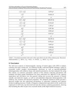
Tables 1 and 2 list the parameter values used for the RO and MSF systems, respectively.

Parameters for RO systems
i, number of ions for ionized solutes 2
R, ideal gas constant, N m / kgmole K 8315

Ms, solute molecular weight 58.8
T, seawater temperature, ºC 25
ρ
b
, brine density, kg/m
3
1060
ρ
p
, pure water density, kg/m
3

1000
μ
p
, permeated stream viscosity, kg/m s
0.9x10
-3

μ
b
, brine viscosity, kg/m s

1.09x10
-3

D, diffusivity coefficient, m
2
/s

1x10
-9

P
swip
, SWIP outled pressure, bar

5
eff
swip
, intake pump efficiency

0.74
eff
hpp
, high pressure pumps efficiency

0.74
eff
ers
, energy recovery system efficiency

0.80
f
c
, load factor

0.90
Table 1. Parameters for RO systems
Desalination, Trends and Technologies

324
Parameters and operating ranges of the particular hollow fiber permeator were taken from
(Al-Bastaki &Abbas, 1999; Voros et al., 1997). These specifications constitute constants and
bounds for some variables of the model.

Parameters for MSF system
T
max
, K 385
Cp
msf
, Kcal/(kg K) 1
TD, m 0.030
Pitch: P
t
1.15
BPE, K 1.9
U, Kcal/m
2
/K/h 2000
λ
, Kcal/Kg
550
Table 2. Parameters for MSF system
The optimization model was implemented in General Algebraic Modeling System: GAMS
(Brooke et al., 1997) at a Pentium 4 of 3.00 GHz. At first, the MINLP solver DICOPT was
implemented to solve the problem. Unfortunately, the solver failed to find even a feasible
solution for most case studies. Then, other resolution strategy was carried out in order to
tackle the problem and obtain the optimal solutions.

Since it involves only 4 integer variables, the problem was solved in 2 steps. Firstly, the
relaxed NLP problem was solved, i.e., the integer variables were relaxed to continuous ones.
Departing from the optimal solution of the relaxed problem, the MINLP was solved by
fixing the integer variables at the nearest integer values and optimizing the remaining
variables. Since the MINLP problem presents a lot of non-convexities, a global search
strategy was also implemented. In fact, for each study case, the previous 2 steps were
repeated starting the optimization search from different initial points, and then, the best
local optimal solution was selected. The generalized reduced gradient algorithm CONOPT
was used as NLP solver. This resolution procedure was successful, providing optimal
solutions in all case studies. The total CPU time required to solve all the cases was 1.87s,
what proves that the proposed procedure is highly efficient and the model is
mathematically good conditioned.
11 case studies were solved for seawater salt concentration going from 35000 ppm up to
45000 ppm. The total production was fixed at 2000m
3
/h with a maximum allowed salt
concentration of 570 ppm.
Table 3 shows the values of the main interconnection variables for the optimal solutions:
feed flow rates, product and internal streams, as well as their salt concentrations.
Table 4 reports design variables and operating conditions for each process for the optimal
solutions.
For seawater salt concentrations between 35000 and 38000 ppm, the optimal solutions do not
include the MSF system. In fact, for these salinities, the optimal hybrid plant designs consist
on a typical two stage RO plant. However, if the seawater salinity is greater than 38000 ppm,
both desalination processes are present in the optimal design of the plant; that is: including
MSF system is profitable.
Figure 5 shows a scheme of the optimal design of the plant obtained for seawater salinities
between 35000 and 38000 ppm.
Optimization of Hybrid Desalination Processes
Including Multi Stage Flash and Reverse Osmosis Systems

325


45000
561.9
1438.1
1947.5
4091.6
-
4546.9
561.9
2599.4
-
-
1385.6
4091.6
1044.6
-
-
3047.2
-
3047.2
393.7
-
-
-
2653.4
55431.6
63247.0

45000
592.1
60220.3
60220.3
1324.8
68959.8
0.9198
44000
496.4
1503.6
1631.7
4144.8
-
4073.0
496.4
2441.3
-
-
1135.3
4144.8
1095.8
-
-
3049.0
-
3049.0
407.8
-
-
-

2641.2
55530.6
63237.4
44000
566.1
59610.0
59610.0
1274.4
68617.4
0.8968
43000
428.8
1571.2
1336.0
4199.9
-
3574.3
428.8
2238.3
-
-
907.2
4199.9
1149.1
-
-
3050.8
-
3050.8
422.1

-
-
-
2628.6
55726.6
63322.7
43000
541.5
58992.1
58992.1
1226.4
68269.1
0.8726
42000
358.5
1641.5
1057.7
4256.7
-
3044.2
358.5
1986.5
-
-
699.2
4256.7
1204.8
-
-
3051.8

-
3051.8
436.8
-
-
-
2615.0
56050.2
63531.0
42000
518.2
58375.5
58375.5
1180.6
67928.1
0.8486
41000
285.9
1714.1
794.6
4315.4
-
2444.1
285.9
1599.3
-
-
558.8
4315.4
1262.4

-
-
3053.0
-
3053.0
451.7
50.2
-
-
2551.2
56833.3
64363.0
41000
496.2
57747.9
57747.9
1137.1
67577.7
0.8240
40000
210.6
1789.4
543.9
4376.8
-
1808.6
210.6
1169.2
-
-

428.7
4376.8
1322.5
-
-
3054.3
-
3054.3
466.9
95.4
-
-
2492.0
58059.1
65712.0
40000
475.3
57113.9
57113.9
1095.3
67221.6
0.7985
39000
132.4
1867.6
304.0
4441.0
-
1146.4
132.4

725.4
-
-
288.6
4441.0
1385.2
-
-
3055.8
-
3055.8
482.4
117.1
-
-
2456.3
60317.6
68194.8
39000
455.4
56472.6
56472.6
1055.3
66861.1
0.7717
38000
-
2000
-
4790.1

-
-
-
-
-
-
-
4790.1
1540.7
-
-
2808.8
440.6
2808.8
459.3
-
-
-
2349.5
-
-
38000
437.8
55810.8
55810.8
1013.6
66522.5
0.7410
37000
-

2000
-
4498.0
-
-
-
-
-
-
-
4498.0
1492.3
-
-
3005.7
-
3005.7
507.7
-
-
-
2498.0
-
-
37000
419.8
55160.9
55160.9
978.9
66174.0

0.7121
36000
-
2000
-
4373.0
-
-
-
-
-
-
-
4373.0
1495.1
-
-
2877.9
-
2877.9
504.9
-
-
-
2373.0
-
-
36000
402.4
54493.6

54493.6
951.6
65884.8
0.6952
35000
-
2000
-
4241.3
-
-
-
-
-
-
-
4241.3
1499.6
-
-
2741.7
-
2741.7
500.4
-
-
-
2241.3
-
-

35000
383.8
53934.2
53934.2
940.5
65764.6
0.6784
F
P
RM
Rro1
Rro2
Rbdw
F
P
RM
Rro1
Rro2
Rbdw
F
P
RM
Rro1
Rro2
Rbdw
F
R
F
P
R

F
P
R
Optimal solutions for the hybrid plant: MSF-RO. Total Production: 2000m
3
/h. Maximum allowed salt concentration: 570pm
Seawater salinity Cfeed,
ppm

Production flow rates for MSF and RO processes
W
msf
P
, m
3
/h
(W
ro1
P
+ W
ro2
P
), m
3
/h
Seawater feed: Wfeed, m
3
/h
MSF
RO1

RO2
Flow rates of the interconnection streams: W, m
3
/h
MSF
MSF
MSF
MSF
MSF
MSF
RO1
RO1
RO1
RO1
RO1
RO1
RO2
RO2
RO2
RO2
RO2
RO2
Salt concentration o
f the interconnection streams: C, ppm
MSF
MSF
RO1
RO1
RO1
RO2

RO2
RO2
Cost of fresh water, $/m
3

Table 3. Optimal solutions for the hybrid plant: interconnection variables
Desalination, Trends and Technologies

326
Optimal solutions for the hybrid plant: MSF-RO. Design variables and operating conditions.
Seawater
salinity:
Cfeed, ppm
35000 36000 37000 38000 39000 40000 41000 42000 43000 44000 45000
MSF
Q
Des
,
Gcal/h
- - - - 8.80 12.93 16.78 20.46 23.89 27.10 30.14
NS
- - - - 19 23 26 28 30 32 33
A
S
, m
2
- - - - 828.8 1103.5 1332.8 1515.5 1679.8 1836.0 1957.8
A
t
, m

2
- - - - 11858.919552.9 27100.3 34308.4 40568.8 46406.2 52594.8
Δt, K
- - - - 7.24 6.75 6.48 6.34 6.30 6.28 6.25
Δt
f
, K
- - - - 3.54 2.95 2.63 2.46 2.34 2.23 2.19
Δt
e
, K
- - - - 1.80 1.89 1.95 1.99 2.07 2.15 2.16
N
t

- - - - 368 501 615 723 798 855 940
L
d
, m - - - - 8.55 12.09 15.13 17.66 19.88 21.96 23.74
Hs, m - - - - 1.45 1.53 1.58 1.63 1.66 1.67 1.72
D
S
, m - - - - 0.45 0.53 0.58 0.63 0.66 0.67 0.72
T
msf
F
, K - - - - 310.5 310.3 310.3 309.9 308.6 307.4 306.3
T
msf
R

, K - - - - 317.7 317.1 316.7 316.2 314.9 313.7 312.6
RO1
NM
1
4633 4777 4915 5232 4843 4773 4706 4642 4580 4520 4462
P
f
1
, atm 67.900 67.900 67.900 67.899 67.900 67.900 67.899 67.900 67.893 67.898 67.900
HPP1 yes yes yes yes yes yes yes yes yes yes yes
T
ro1
, K

298.0 298.0 298.0 298.0 298.0 298.0 298.0 298.0 298.0 298.0 298.0
RO2
NM
2
3129 3189 3286 3063 3332 3331 3330 3328 3327 3325 3323
P
f
2
, atm 67.868 67.868 67.868 67.866 67.867 67.867 67.867 67.867 67.860 67.865 67.866
HPP2 no no no no no no no no no no no
T
ro2
, K 298.0 298.0 298.0 298.0 298.0 298.0 298.0 298.0 298.0 298.0 298.0
Table 4. Optimal solutions for the hybrid plant: design variables and operating conditions

Fig. 5. Scheme of the optimal design for seawater salinities between 35000 and 38000 ppm
The stream with flow rate W
ro1
Rbdw
is only present for 38000 ppm of seawater salinity. For
salinities lower than 38000 ppm, the totality of the stream rejected from the first RO stage:
system RO1, enters into the second RO stage: system RO2. Then, the stream entering into
the system RO2 is sufficiently pressurized. Therefore, the high pressure pumps before
system RO2 are avoided in the optimal solutions. This decision is properly made by the
optimization procedure, and it is correctly reflected in the cost function.
RO2
SWIP
Wfeed
ro1
ro2
F
W
ro1
F
W
RO1
ro2
P
W
ro1
Rro2
W
ro1
P
W

ERS
ro2
Rbdw
W
ro1
Rbdw
W
PRODUCT
HPP1
Optimization of Hybrid Desalination Processes
Including Multi Stage Flash and Reverse Osmosis Systems

327
Figure 6 shows a scheme of the optimal solutions obtained for seawater salt concentrations
between 39000 and 45000 ppm.
For these case studies, both desalination processes are present at the optimal hybrid plant
design. The RO systems work as a two-stage RO plant, i.e.: system RO1 is fed directly from
sea, while its rejected stream is the fed stream for system RO2. No other streams are blended
to feed RO systems.
Regarding MSF system, it operates with an important recycle. This re-circulated stream
reduces the chemical pre-treatment and raises the feed stream temperature with the
consequent reduction of external heat consumption. Both factors straightly impact on the
final cost.


Fig. 6. Scheme of the optimal design for seawater salinities between 39000 and 45000 ppm
As it is also shown in Table 3, the three first cases presented in Figure 6 include the stream
with flow rate W
ro2
RM

. However, for seawater salt concentrations higher than 41000 ppm this
flow rate is null and the stream does not exist. Then, for the last four case studies, even
though the two desalination processes are selected for the optimal plant design, they operate
in independent way. In fact: there is no stream connecting the MSF and RO processes.
However, both processes share the intake and pre-treatment system. Furthermore, the
salinity of the product stream satisfies the maximum allowed salt concentration requirement
because the three product streams are blended. As it can be seen at Table 3, if only the
permeate streams coming from RO systems are blended, then the salt concentration of the
resulting stream will be far above the maximum allowed salt concentration.
Again, the stream feeding system RO2 is composed only by the stream rejected from system
RO1 and it is high pressurized. Thus, the high pressure pumps before system RO2 are
unnecessary and consequently, they are avoided at the optimal design.
Figure 7 shows the fresh water produced by each desalination process for all the case
studies.
As it was mentioned, for seawater salt concentrations below 38000 ppm, MSF system is not
present, thus the demand is totally satisfied by RO systems. On the other hand, for seawater
salinities higher than 38000 ppm, both processes contribute to satisfy the demand. Although
the RO systems produce more fresh water than MSF system, the MSF production increases
according to the seawater salinity rise.
SWIP
Wfeed
msf
Wfeed
ro1
msf
F
W
ro2
F
W

ro1
F
W
MSF
HPP1
RO2
RO1
msf
RM
W
msf
Rbdw
W
msf
P
W
ro2
P
W
ro1
Rro2
W
ro1
P
W
ERS
ro2
Rbdw
W
ro2

RM
W
PRODUCT
Desalination, Trends and Technologies

328



Fig. 7. Fresh water production
If the MSF system would not be considered, for the optimal design of a two stage RO plant
the capacity of the second stage will decrease when the seawater salinity increases
(Marcovecchio et al., 2005). In fact, even though the stream rejected from the first RO stage is
high pressurized and it could enter into a second stage with no need of high pressure
pumps; in the optimal design, part of this stream is discharged back to the sea. The second
stage capacity will continue decreasing until only one RO stage is the optimal design for
high feed salt concentration. The reason why it is no longer profitable to use the stream
rejected from the first RO stage is that its salinity is too high. Thus, the salt concentration of
the potential permeate will be lower but also high and then, it is not possible to satisfy the
maximum allowed salt concentration even by blending with the first stage permeate.
Therefore, the fresh water produced by the first stage must be higher in order to satisfy the
demand. Consequently, the flow rate of seawater is increased. As a consequence, the cost
per m
3
of fresh water increases, since many costs are directly affected.
Contrary, in a hybrid plant where the MSF process is available, in that break point where the
optimal design of a RO plant changes, it begins to be profitable to complement the RO
production with distillated from MSF system.
Then, for feed salinities higher than 38000 ppm, the growth of MSF system production is
approximately linear. With this plant design, there is no stream rejected from the first RO

stage being discharged back to the sea, i.e. the totality of that stream enters into the second
RO stage. And the total production of the plant reaches the requirement of maximum
allowed salt concentration by blending the slightly concentrated permeate from RO systems
with the free of salt distillate of MSF process.
Finally, Figure 8 compares the cost per m
3
of fresh water produced with the optimal
configurations obtained for the hybrid plant with those obtained for the RO stand alone
plant.
As it is shown in Figure 8, the cost reduction reached with the hybrid RO-MSF plant is
considerable. For feed salinities between 39000 and 44000 ppm, the cost function has an

Optimization of Hybrid Desalination Processes
Including Multi Stage Flash and Reverse Osmosis Systems

329

Fig. 8. Fresh water cost for hybrid RO-MSF plants and RO stand alone plants
almost linear growth with respect to the seawater salinity, for both: RO and hybrid plant.
However, the growth rate associated to the hybrid plant cost is far lower.
For comparative purposes, optimal designs for the MSF stand alone plant were calculated.
That is, it was calculated the cost per m
3
of fresh water produced by the MSF-once through
process satisfying the same demand: 2000 m
3
/h. In the implemented model, this cost is not
affected by the feed salinity. The cost obtained for the case studies was $1.1683. Also, the
designs obtained are the same for all the case studies, since the only constraint that could
affect the solution is the one requiring that the concentration of the stream discharged back

to sea be lower than 67000 ppm, but this limit is not reached in any case.

5. Conclusion
In this work, a MINLP mathematical model for the optimal synthesis and design of hybrid
desalination plants, including the two conversion processes: reverse osmosis and multiple
stage flash evaporation, was presented.
The MSF model is based on a previous work presented by (Mussati et al., 2004). It involves
real-physical constraints for the evaporation process and is derived on energy, mass and
momentum balances. In addition, geometric dimensions of stages including chambers and
pre-heaters are considered as optimization variables. Heat exchange areas of condensers are
also design variables to be determined.
The RO model with hollow fiber permeators is based on the work (Marcovecchio et al.,
2005). For this model, the transport phenomena of solute and water through the membrane
are modelled by Kimura-Sourirajan model. The concentration polarization phenomenon is
taken into account. The Hagen-Poiseuille and Ergun equations are employed to calculate the
pressure drops. In the RO model, the number of permeators operating in parallel, the
operating pressure and flow rates are the main optimization variables.
The modelled hybrid plant includes two RO and one MSF systems. The proposed
superstructure allows optimizing not only operating conditions but also process
configurations simultaneously. Thus, the model includes network constraints which are
related to all potential interconnections between the three systems.
Desalination, Trends and Technologies

330
Network constraints ensure the correct definition of flow rates, salt concentrations and
temperatures for each stream.
Cost equations take into account all the factors affecting the cost of each process. Certainly,
capital investment and operating cost of all process equipments were considered.
Optimal solutions for eleven case studies were obtained, for different seawater salinities.
Then optimal designs and operating conditions were determined by minimizing the cost per

m
3
of produced fresh water. Cost equations are able to reflect accurately the presence or
absence of certain equipment, stream or even a whole system.
From the optimal solutions, it can be concluded that the RO stand alone plant is the best
option for feed salinities between 35000 and 38000 ppm. In fact, the optimal design obtained
for these cases consist on a two-stage RO plant while the MSF process was completely
eliminated.
However, when the seawater salinity rises, it is profitable to integrate the MSF system in a
hybrid plant. Actually, for feed salinities higher than 38000 ppm both desalination processes
are present at the optimal plant design. In these cases, the integration of MSF process allows
a better use of the rejected streams leaving the first and second RO stages. As a consequence,
the final fresh water cost is reduced. It is important to note that although the RO production
is higher than the MSF one, the MSF capacity increases according to the seawater salinity
rise.
Then, important conclusions about the relationship between membrane and thermal
desalination processes can be established from the optimal solutions presented in this work.
In fact, the optimal hybrid plants were described for different seawater conditions, in order
to minimize the cost of producing fresh water.
In future works, more detailed models for each process will be included in the
superstructure problem, in order to improve the model presented here. In addition, other
interconnections between the two studied processes will be considered, as the incorporation
of streams coming from RO system in different stages of the MSF evaporator. Then, the
interaction between both desalination processes will be more flexible and may lead to
reduce the total cost of the process.
6. Acknowledgements
The authors acknowledge financial support from ‘Agencia Nacional de Promoción
Científica y Tecnológica’ (ANCyT), and ‘Consejo de Investigaciones Científicas y Técnicas’
(CONICET), Argentina.
7. Nomenclature

Subscripts
msf Multi Stage Flash System
ro1 Reverse Osmosis System 1
ro2 Reverse Osmosis System 2
Superscripts
F Feed
P Permeate – Product
Optimization of Hybrid Desalination Processes
Including Multi Stage Flash and Reverse Osmosis Systems

331
R Rejected – Concentrated brine
Rbdw Rejected to be blown down
RM Rejected brine entering into MSF system
Rro1 Rejected brine entering into RO1 system
Rro2 Rejected brine entering into RO1 system

ρ
b
brine density - RO, kg / m
3
ρ
p
pure water density - RO, kg / m
3
μ
b
brine viscosity - RO, kg / (m s)
μ
p

permeated stream viscosity - RO, kg / (m s)
λ
latent heat evaporation – MSF, Kcal / kg
Q
f
feed flow rate per membrane module - RO, m
3
/h
Q
p
permeate flow rate per membrane module - RO, m
3
/h
Q
b
brine flow rate inside the shell per membrane module - RO, m
3
/h
C
m
salt concentration at the membrane wall - RO, ppm
ρ
vap
vapor density – MSF, kg / m
3
Δt temperature drop – MSF, K
J
w
water flux - RO, kg/m
2

.h
J
S
solute flux - RO, kg/m
2
.h
ε void fraction - RO
Δt
e
effective driving force for the heat transfer operation – MSF, K
Δt
f
temperature drop for the flashing operation – MSF, K
P
f
feed stream pressure - RO, atm
p
P Average pressure in the fiber bore - RO, atm
b
P Average pressure on the shell side of the fiber bundle - RO, atm
V
w
velocity of permeation flow - RO, m/h
U
so
Superficial velocity at the outer radius of the fiber bundle - RO, m/s
U
si
Superficial velocity at the inner radius of the fiber bundle - RO, m/s
U

S
superficial velocity in the radial direction of the bulk stream - RO, m/s
A
pure water permeability constant - RO, kg/m
2
.s.atm
A
m
module membrane area - RO, m
2

AOC Annual operating cost, $/y
A
S
Total stage surface area – MSF, m
2

A
t
total heat transfer area – MSF, m
2

B solute permeability constant - RO, m/s
B
msf
chamber width – MSF, m
BPE boiling point elevation, K
C salt concentration, ppm
cc
area

capital cost of heat transfer area of MSF system, $
cc
cw
capital cost of civil work, $
cc
eq
total equipment cost, $
cc
ers
capital cost for the Energy Recovery System, $
cc
hpp1
capital cost of High Pressure Pumps for system RO1, $
cc
hpp2
capital cost of High Pressure Pumps for system RO2, $
Desalination, Trends and Technologies

332
cc
i
indirect capital cost, $
cc
swip
capital cost for the Seawater Intake and Pre-treatment system, $
Cfeed feed salt concentration, ppm
c
max
maximum salt concentration allowed for the product stream, ppm
co

c
capital charge cost, $/year
co
ch
chemical treatment cost, $/year
co
e
energy cost, $/year
co
ht
cost of the heat consumed by system MSF, $/year
co
om
general operation and maintenance cost, $/year
co
pw
power cost for system MSF, $/year
co
rp
cost of permeator replacement, $/year
co
s
spares cost, $/year
cost cost per m
3
of produced fresh water, $/m
3

Cp
msf

heat capacity – MSF, Kcal / (kg K)
crf capital recovery factor
D diffusivity coefficient - RO, m
2
/ s
d
p
specific surface diameter - RO, m
Ds shell diameter – MSF, m
eff
ers
energy recovery system efficiency
eff
hpp
high pressure pumps efficiency
eff
swip
intake pump efficiency
f
c
load factor
Hs chamber height – MSF, m
i number of ions for ionized solutes - RO
k mass transfer coefficient - RO, m/s
L length of fiber bundle - RO, m
Lb level of brine in the flashing chamber – MSF, m
L
d
length of desaltor – MSF, m
Ms solute molecular weight – RO

NM number of membrane module operating in parallel mode in each RO system
N
rt
number of rows in the vertical direction – MSF
NS number of flashing stages – MSF
N
t
number of tubes – MSF
P
in
pressure of the stream entering into each RO system – RO, atm
prodc total plant production, m
3
/h
P
swip
seawater intake system outlet pressure, bar
P
t
Pitch – MSF
Q
Des
external heat consumption – MSF, Gcal/h
R ideal gas constant - RO, N m / (kgmol K)
Re Reynolds number (2.r
0.
U
s
S
.

ρ
b
/
μ
b
) - RO
R
i
inner radius of the fiber bundle - RO, m
r
i
inner fiber radius - RO, m
R
o
outer radius of the fiber bundle - RO, m
r
o
outer fiber radius - RO, m
Optimization of Hybrid Desalination Processes
Including Multi Stage Flash and Reverse Osmosis Systems

333
Sc Schmidt number (
μ
b
/
ρ
b
.D) - RO
Sh Sherwood number (2.k.r

o
/D) - RO
T temperature, K
TCC total capital cost, $
TD tube diameter – MSF, m
Tfeed seawater temperature, K
T
max
maximum brine temperature – MSF, K
U overall heat transfer coefficient – MSF, Kcal / (K m
2
h)
V
vap

vapor velocity – MSF, m / s
W flow rate, m
3
/h
Wfeed seawater feed flow, m
3
/ h
8. References
Agashichev, S.P. (2004). Analysis of integrated co-generative schemes including MSF, RO
and power generating systems (present value of expenses and “levelised” cost of
water).
Desalination, 164 (3): 281-302, ISSN: 0011-9164.
Al-Bastaki, N.M. & Abbas, A. (1999). Modeling an industrial reverse osmosis unit.
Desalination 126 (1-3): 33-39, ISSN: 0011-9164.
Brooke, A.; Kendrick, D.; Meeraus, A. & Raman, R. (1997). GAMS Language Guide, Release

2.25, Version 92. GAMS Development Corporation.
Cardona, E. & Piacentino, A. (2004). Optimal design of cogeneration plants for seawater
desalination.
Desalination 166: 411-426, ISSN: 0011-9164.
Helal, A.M.; El-Nashar, A.M.; Al-Katheeri, E. & Al-Malek, S. (2003). Optimal design of
hybrid RO/MSF desalination plants. Part I: Modeling and algorithms.
Desalination
154 (1): 43-66, ISSN: 0011-9164.
Kimura, S. & Sourirajan, S. (1967). Analysis of data in reverse osmosis with porous cellulose
acetate membranes.
AIChE Journal 13 (3): 497-503, ISSN: 1547-5905.
Malek, A.; Hawlader, M.N.A. & Ho, J.C. (1996). Design and economics of RO seawater
desalination.
Desalination 105 (3): 245-261, ISSN: 0011-9164.
Marcovecchio, M.G.; Aguirre, P.A. & Scenna, N.J. (2005). Global optimal design of reverse
osmosis networks for seawater desalination: modeling and algorithm.
Desalination
184 (1-3): 259-271, ISSN: 0011-9164.
Marcovecchio, M.G.; Mussati, S.F.; Aguirre, P.A. & Scenna, N.J. (2005). Optimization of
hybrid desalination processes including multi stage flash and reverse osmosis
systems.
Desalination 182 (1-3): 111-122, ISSN: 0011-9164.
Marcovecchio, M.G.; Mussati, S.F.; Scenna, N.J. & Aguirre, P.A. (2009).
Global optimal
synthesis of integrated hybrid desalination plants,
Computer Aided Chemical
Engineering
, Vol 26: 573-578, ISBN-13: 978-0-444-53433-0. Elsevier Science B.V. 19
th

European Symposium on Computer Aided Process Engineering (ESCAPE19), 14-17
June 2009. Cracow, Poland.
Mussati, S.F. ; Aguirre, P.A. & Scenna, N.J. (2006). Superstructure of alternative
Configurations of the multistage flash desalination process.
Industrial & Engineering
Chemistry Research
45 (21): 7190-7203, ISSN: 0888-5885.
Desalination, Trends and Technologies

334
Mussati, S.F.; Marcovecchio, M.G.; Aguirre, P.A. & Scenna, N.J. (2004). A new global
optimization algorithm for process design: its application to thermal desalination
processes.
Desalination 166: 129-140, ISSN: 0011-9164.
Voros, N.G. ; Maroulis, Z.B. & Marinos-Kouris, D. (1997). Short-cut structural design of
reverse osmosis desalination plants.
Journal of Membrane Science 127 (1): 47-68, ISSN:
0376-7388.
Wade, N.M. (2001). Distillation plant development and cost update.
Desalination 136 (1-3): 3-
12, ISSN: 0011-9164.