Discrete Time Systems Part 12 ppt
Bạn đang xem bản rút gọn của tài liệu. Xem và tải ngay bản đầy đủ của tài liệu tại đây (734.4 KB, 30 trang )
Uncertain Discrete-Time Systems with Delayed State:
Robust Stabilization with Performance Specification via LMI Formulations
providing an H ∞ guaranteed cost γ =
signal w k .
√
319
μ between the output ek , as defined by (93), and the input
Proof. The proof follows similar steps to those of the proof of the Theorem 4. Once (94) is
F11 F12
is assured by the block
verified, then the regularity of F =
F22 Λ F22
˜
Pi − F − F T =
T ˜
T
˜
P11i − F11 − F11 P12i − F12 − Λ T F22
˜22i − F22 − F T
P
22
< 0.
Thus it is possible to define the congruence transformation TH given by (53) with
T = I3 ⊗ F − T = I3 ⊗
F11 F12
F22 Λ F22
−T
¯ T
ˆ
ˆ
to get Ψi = TH Ψi TH . In block (7, 7) of Ψi , it always exist a real scalar κ ∈]0, 2[ such that for
θ ∈]0, 1], κ (κ − 2) = − θ. Thus, replacing this block by κ (κ − 2)I p , the optimization variables
W and Wd by K F22 and Kd F22 , respectively, and using the definitions given by (91)–(93) it
˜ ˜
ˆ ˆ
ˆ
˜ ˜
is possible to verify (36) by i) replacing matrices Ai , Adi , Ci , Cdi , Bwi and Dwi by Ai , Adi , Ci ,
ˆ
ˆ
ˆ
Cdi , Bwi and Dwi , respectively, given in (93); ii) choosing G = 1 I p that leads block (7, 7) to be
κ
rewritten as in (55); iii) assuming
Pi =
F11 F12
F22 Λ F22
−T
˜
˜
P11i P12i
˜
P22i
Qi =
F11 F12
F22 Λ F22
−T
˜
˜
Q11i Q12i
˜
Q22i
and
⎡
F11 F12
⎢
⎢ F22 Λ F22
⎢
0
⎢
XH = ⎢
0
⎢
⎢
⎢
0
⎣
0
−1
F11 F12
F22 Λ F22
F11 F12
F22 Λ F22
−1
−1
⎤
0 ⎥
⎥
⎥
0 ⎥
⎥
0 ⎥
1 ⎥
Ip ⎥
⎦
κ
0
which completes the proof.
An important aspect of Theorem 7 is the choice of Λ ∈ R n×nm in (94). This matrix plays
an important role in this optimization problem, once it is used to adjust the dimensions of
block (2, 1) of F that allows to use F22 to design both robust state feedback gains K and Kd .
This kind choice made a priori also appears in some results found on the literature of filtering
theory. Another possibility is to use an interactive algorithm to search for a better choice of Λ.
This can be done by taking the following steps:
1. Set max_iter←− maximum number of iterations; j ←− 0;
=precision;
2. Choose an initial value of Λ j ←− Λ such that (94) is feasible.
(a) Set μ j ←− μ; Δμ ←− μ j ; F22,j ←− F22 ; Wj ←− W; Wd,j ←− Wd .
3. While (Δμ > )AND(j < max_iter)
320
Discrete Time Systems
(a) Set j ←− j + 1;
(b) If j is odd
i. Solve (94) with F22 ←− F22,j ; W ←− Wj ; Wd ←− Wd,j .
ii. Set Λ ←− Λ j ;
Else
i. Solve (94) with Λ ←− Λ j .
ii. Set F22,j ←− F22 ; Wj ←− W; Wd,j ←− Wd .
End_if
(c) Set μ j ←− μ; Δμ ←− |(μ j − μ j−1 )|;
End_while
4. Calculate K and Kd by means of (95);
5. Set μ = μ j
Once this is a non-convex algorithm — only steps 3.(b).i are convex — different initial guesses
√
for Λ may lead to different final values for the controllers K and Kd , as well as to the γ = μ
To overcome the main drawback of this proposal, two approaches can be stated. The first
follows the ideas of Coutinho et al. (2009) by designing an external loop to the closed-loop
system proposed in Figure 6. In this sense, it is possible to design a transfer function that can
adjust the gain and zeros of the controlled system. The second approach is based on the work
of Rodrigues et al. (2009) where a dynamic output feedback controller is proposed. However,
in this case the achieved conditions are non-convex and a relaxation algorithm is required.
In the example presented in the sequel, Theorem 7 with
Λ=
In m
0n−nm ×nm
(96)
Example 5. Consider the uncertain discrete-time system with time-varying delay dk ∈ I[2, 13] as
given in (1) with uncertain matrices belonging to polytope (2)-(3) with 2 vertices given by
A1 =
0.6 0
,
0.35 0.7
Bw1 =
Ad1 =
0
,
1
C1 = 1 0 ,
Dw1 = 0.2,
B1 =
0.1 0
,
0.2 0.1
0
,
1
Bw2 = 1.1Bw1 ,
Cd1 = 0 0.05 ,
D1 = 0.1,
A2 = 1.1A1 ,
C2 = 1.1C1 ,
Dw2 = 1.1Dw1
Ad2 = 1.1Ad1
B2 = 1.1B1
Cd2 = 1.1Cd1
D2 = 1.1D1
(97)
(98)
(99)
(100)
It is desired to design robust state feedback gains for control law (6) such that the output of this
uncertain system approaches the behavior of delay-free model given by
Ωm = G (z) =
0.1847z − 0.01617
=
z + 0.3
−0.3
0.25
−0.2864 0.1847
(101)
Thus, it is desired to minimize the H ∞ guaranteed cost between signals e k and wk identified in Figure 6.
The static gain of model (101) was adjusted to match the gain of the controlled system. This procedure
is similar to what has been proposed by Coutinho et al. (2009). The choice of the pole and the zero was
arbitrary. Obviously, different models result in different value of H ∞ guaranteed cost.
Uncertain Discrete-Time Systems with Delayed State:
Robust Stabilization with Performance Specification via LMI Formulations
321
By applying Theorem 7 to this problem, with Λ given in (96), it has been found an H ∞ guaranteed cost
γ = 0.2383 achieved with the robust state feedback gains:
K = 1.8043 −0.7138
and
Kd = −0.1546 −0.0422
(102)
In case of unknown dk , Theorem 7 is unfeasible for the considered variation delay interval, i.e., imposing
Kd = 0. On the other hand, if this interval is narrower, this system can be stabilized with an H ∞
¯
¯
guaranteed cost using only the current state. So, reducing the value of d from d = 13, it has been found
that Theorem 7 is feasible for dk ∈ I[2, 10] with
K = −2.7162 −0.6003
and
Kd = 0
(103)
and γ = 0.3427. Just for a comparison, with this same delay interval, if K and Kd are designed, then
the H ∞ guaranteed cost is reduced about 37.8% yielding an attenuation level given by γ = 0.2131.
Thus, it is clear that, whenever the information about the delay is used it is possible to reduce the
H∞ guaranteed cost. Some numerical simulations have been done considering gains (102), and a
disturbance input given by
0, if k = 0 or k ≥ 11
(104)
wk =
1, if 1 ≤ 10
Two conditions were considered: i) dk = 13, ∀k ≤ 0 and different values of α1 ∈ [0, 1]; and ii)
dk = d =∈ I[2, 13] with α1 = 1 (i.e., only for the first vertex). The output responses of the controlled
system have been performed with dk = 13, ∀k ≥ 0. This family of responses and that of the reference
model are shown at the top of Figure 7 with solid lines. A red dashed line is used to indicate the desired
model response. The absolute value of the error (| ek | = | yk − ymk |) is shown in solid lines at the
bottom of Figure 7 and the estimate H ∞ guaranteed cost provide by Theorem 7 in dashed red line. The
respective control signals are shown in Figure 8.
The other set of time simulations has been performed using only vertex number 1 (α1 = 1). In this
numerical experiment, the perturbation (104) has been applied to system defined by vertex 1 and twelve
numerical simulations were performed, one for each constant delay value dk = d ∈ [2, 13]. The results
are shown in Figure 9: at the top, a red dashed line indicates the model response and at the bottom it is
shown the absolute value of the error (| ek | = | yk − ymk |) in solid lines and the estimate H ∞ guaranteed
cost provide by Theorem 7 in dashed red line. This value is the same provide in Figure 7, once it is the
same design. The respective control signals performed in simulations shown in Figure 9 are shown in
Figure 10.
At last, the frequency response considering the input wk and the output ek is shown in Figure 11 with
a time-invariant delay. For each value of delay in the interval [2, 13] and α ∈ [0, 1], a frequency
sweep has been performed on both open loop and closed-loop systems. The gains used in the closed-loop
system are given in (102). It is interesting to note that, once it is desired that yk approaches ymk , i.e.,
ek approaches zero, the gain frequency response of the closed-loop should approaches zero. By Figure 11
the H ∞ guaranteed cost of the closed-loop system with time invariant delay is about 0.1551, but this
value refers to the case of time-invariant delay only. The estimative provided by Theorem 7 is 0.2383
and considers a time varying delay.
6. Final remarks
In this chapter, some sufficient convex conditions for robust stability and stabilization
of discrete-time systems with delayed state were presented. The system considered is
uncertain with polytopic representation and the conditions were obtained by using parameter
dependent Lyapunov-Krasovskii functions. The Finsler’s Lemma was used to obtain LMIs
322
Discrete Time Systems
0.3
0.2
yk 0.1
0
−0.1
0
5
10
15
20
25
30
35
40
45
50
30
35
40
45
50
k
0.3
0.25
0.2
|e k | 0.15
0.1
0.05
0
0
5
10
15
20
25
k
Fig. 7. Time behavior of yk and | ek | in blue solid lines and model response (top) and
estimated H ∞ guaranteed cost (bottom) in red dashed lines, for dk = 13 and α ∈ [0, 1].
0.5
0
uk
−0.5
−1
0
5
10
15
20
25
30
35
40
45
50
k
Fig. 8. Control signals used in time simulations presented in Figure 7.
condition where the Lyapunov-Krasovskii variables are decoupled from the matrices of the
system. The fundamental problem of robust stability analysis and stabilization has been dealt.
The H ∞ guaranteed cost has been used to improve the performance of the closed-loop system.
It is worth to say that even all matrices of the system are affected by polytopic uncertainties,
the proposed design conditions are convex, formulated in terms of LMIs.
It is shown how the results on robust stability analysis, synthesis and on H ∞ guaranteed cost
estimation and design can be extended to match some special problems in control theory such
Uncertain Discrete-Time Systems with Delayed State:
Robust Stabilization with Performance Specification via LMI Formulations
323
0.25
0.2
0.15
yk
0.1
0.05
0
−0.05
−0.1
0
5
10
15
20
25
30
35
40
45
50
30
35
40
45
50
k
0.3
0.25
0.2
|e k |0.15
0.1
0.05
0
0
5
10
15
20
25
k
Fig. 9. Time behavior of yk and | ek | in blue solid lines and model response (top) and estimated
H∞ guaranteed cost (bottom) in red dashed lines, for vertex 1 and delays from 2 to 13.
0.2
0
−0.2
uk
−0.4
−0.6
−0.8
0
5
10
15
20
25
30
35
40
45
50
k
Fig. 10. Control signals used in time simulations presented in Figure 9.
as decentralized control, switched systems, actuator failure, output feedback and following
model conditions.
It has been shown that the proposed convex conditions can be systematically obtained by
i) defining a suitable positive definite parameter dependent Lyapunov-Krasovskii function;
ii) calculating an over bound for ΔV (k) < 0 and iii) applying Finsler’s Lemma to get a set
of LMIs, formulated in a enlarged space, where cross products between the matrices of the
system and the matrices of the Lyapunov-Krasovskii function are avoided. In case of robust
design conditions, they are obtained from the respective analysis conditions by congruence
transformation and, in the H ∞ guaranteed cost design, by replacing some matrix blocs by
their over bounds. Numerical examples are given to demonstrated some relevant aspects of
the proposed conditions.
324
Discrete Time Systems
0.7
open loop
0.6
0.5
0.4
E(z)
W (z)
0.3
0.2
0.1
0
0
0.5
1
1.5
2
2.5
3
3.5
0
0.5
1
1.5
2
2.5
3
3.5
ω[rad/s]
0.7
closed-loop
0.6
0.5
0.4
E(z)
W (z)
0.3
0.2
0.1
0
ω[rad/s]
Fig. 11. Gain frequency response between signals ek and wk for the open loop (top) and
closed-loop (bottom) cases for delays from 2 to 13 and a sweep on α ∈ [0, 1].
The approach used in this proposal can be used to deal with more complete
Lyapunov-Krasovskii functions, yielding less conservative conditions for both robust stability
analysis and design, including closed-loop performance specifications as presented in this
chapter.
7. References
Boukas, E.-K. (2006). Discrete-time systems with time-varying time delay: stability and
stabilizability, Mathematical Problems in Engineering 2006: 1–10.
Chen, W. H., Guan, Z. H. & Lu, X. (2004). Delay-dependent guaranteed cost control for
uncertain discrete-time systems with both state and input delays, Journal of The
Franklin Institute 341(5): 419–430.
Chu, J. (1995). Application of a discrete optimal tracking controller to an industrial electric
heater with pure delays, Journal of Process Control 5(1): 3–8.
Coutinho, D. F., Pereira, L. F. A. & Yoneyama, T. (2009). Robust H2 model matching from
frequency domain specifications, IET Control Theory and Applications 3(8): 1119–1131.
de Oliveira, M. C. & Skelton, R. E. (2001). Stability tests for constrained linear systems, in
S. O. Reza Moheimani (ed.), Perspectives in Robust Control, Vol. 268 of Lecture Notes in
Control and Information Science, Springer-Verlag, New York, pp. 241–257.
de Oliveira, P. J., Oliveira, R. C. L. F., Leite, V. J. S., Montagner, V. F. & Peres, P. L. D. (2002).
LMI based robust stability conditions for linear uncertain systems: a numerical
comparison, Proceedings of the 41st IEEE Conference on Decision and Control, Las Vegas,
pp. 644–649.
Uncertain Discrete-Time Systems with Delayed State:
Robust Stabilization with Performance Specification via LMI Formulations
325
Du, D., Jiang, B., Shi, P. & Zhou, S. (2007). H ∞ filtering of discrete-time switched systems
with state delays via switched Lyapunov function approach, IEEE Transactions on
Automatic Control 52(8): 1520–1525.
Fridman, E. & Shaked, U. (2005a). Delay dependent H ∞ control of uncertain discrete delay
system, European Journal of Control 11(1): 29–37.
Fridman, E. & Shaked, U. (2005b). Stability and guaranteed cost control of uncertain discrete
delay system, International Journal of Control 78(4): 235–246.
Gao, H., Lam, J., Wang, C. & Wang, Y. (2004). Delay-dependent robust output feedback
stabilisation of discrete-time systems with time-varying state delay, IEE Proceedings
— Control Theory and Applications 151(6): 691–698.
Gu, K., Kharitonov, V. L. & Chen, J. (2003). Stability of Time-delay Systems, Control Engineering,
Birkhäuser, Boston.
He, Y., Wu, M., Liu, G.-P. & She, J.-H. (2008). Output feedback stabilization for a
discrete-time system with a time-varying delay, IEEE Transactions on Automatic
Control 53(11): 2372–2377.
Hetel, L., Daafouz, J. & Iung, C. (2008). Equivalence between the Lyapunov-Krasovskii
functionals approach for discrete delay systems and that of the stability conditions
for switched systems, Nonlinear Analysis: Hybrid Systems 2: 697–705.
Ibrir, S. (2008). Stability and robust stabilization of discrete-time switched systems with
time-delays: LMI approach, Applied Mathematics and Computation 206: 570–578.
Kandanvli, V. K. R. & Kar, H. (2009). Robust stability of discrete-time state-delayed systems
with saturation nonlinearities: Linear matrix inequality approach, Signal Processing
89: 161–173.
Kapila, V. & Haddad, W. M. (1998). Memoryless H ∞ controllers for discrete-time systems with
time delay, Automatica 34(9): 1141–1144.
Kolmanovskii, V. & Myshkis, A. (1999). Introduction to the Theory and Applications of
Functional Differential Equations, Mathematics and Its Applications, Kluwer Academic
Publishers.
Leite, V. J. S. & Miranda, M. F. (2008a). Robust stabilization of discrete-time systems with
time-varying delay: an LMI approach, Mathematical Problems in Engineering pp. 1–15.
Leite, V. J. S. & Miranda, M. F. (2008b). Stabilization of switched discrete-time systems with
time-varying delay, Proceedings of the 17th IFAC World Congress, Seul.
Leite, V. J. S., Montagner, V. F., de Oliveira, P. J., Oliveira, R. C. L. F., Ramos, D. C. W. & Peres,
P. L. D. (2004). Estabilidade robusta de sistemas lineares através de desigualdades
matriciais lineares, SBA Controle & Automaỗóo 15(1).
Leite, V. J. S. & Peres, P. L. D. (2003). An improved LMI condition for robust D -stability of
uncertain polytopic systems, IEEE Transactions on Automatic Control 48(3): 500–504.
Leite, V. S. J., Tarbouriech, S. & Peres, P. L. D. (2009). Robust H ∞ state feedback control of
discrete-time systems with state delay: an LMI approach, IMA Journal of Mathematical
Control and Information 26: 357–373.
Liu, X. G., Martin, R. R., Wu, M. & Tang, M. L. (2006). Delay-dependent robust stabilisation of
discrete-time systems with time-varying delay, IEE Proceedings — Control Theory and
Applications 153(6): 689–702.
Ma, S., Zhang, C. & Cheng, Z. (2008). Delay-dependent robust H ∞ control for uncertain
discrete-time singular systems with time-delays, Journal of Computational and Applied
Mathematics 217: 194–211.
326
Discrete Time Systems
Mao, W.-J. & Chu, J. (2009). D -stability and D -stabilization of linear discrete time-delay
systems with polytopic uncertainties, Automatica 45(3): 842–846.
Montagner, V. F., Leite, V. J. S., Tarbouriech, S. & Peres, P. L. D. (2005). Stability and
stabilizability of discrete-time switched linear systems with state delay, Proceedings
of the 2005 American Control Conference, Portland, OR.
Niculescu, S.-I. (2001). Delay Effects on Stability: A Robust Control Approach, Vol. 269 of Lecture
Notes in Control and Information Sciences, Springer-Verlag, London.
Oliveira, R. C. L. F. & Peres, P. L. D. (2005). Stability of polytopes of matrices via affine
parameter-dependent Lyapunov functions: Asymptotically exact LMI conditions,
Linear Algebra and Its Applications 405: 209–228.
Phat, V. N. (2005). Robust stability and stabilizability of uncertain linear hybrid systems with
state delays, IEEE Transactions on Circuits and Systems Part II: Analog and Digital Signal
Processing 52(2): 94–98.
Richard, J.-P. (2003). Time-delay systems: an overview of some recent advances and open
problems, Automatica 39(10): 1667–1694.
Rodrigues, L. A., Gonỗalves, E. N., Leite, V. J. S. & Palhares, R. M. (2009). Robust
reference model control with LMI formulation, Proceedings of the IASTED International
Conference on Identification, Control and Applications, Honolulu, HW, USA.
Shi, P., Boukas, E. K., Shi, Y. & Agarwal, R. K. (2003). Optimal guaranteed cost control
of uncertain discrete time-delay systems, Journal of Computational and Applied
Mathematics 157(2): 435–451.
Silva, L. F. P., Leite, V. J. S., Miranda, M. F. & Nepomuceno, E. G. (2009). Robust D -stabilization
with minimization of the H ∞ guaranteed cost for uncertain discrete-time systems
with multiple delays in the state, Proceedings of the 49th IEEE Conference on Decision
and Control, IEEE, Atlanta, GA, USA. CD ROM.
Srinivasagupta, D., Schättler, H. & Joseph, B. (2004). Time-stamped model predictive
previous control: an algorithm for previous control of processes with random delays,
Computers & Chemical Engineering 28(8): 1337–1346.
Syrmos, C. L., Abdallah, C. T., Dorato, P. & Grigoriadis, K. (1997). Static output feedback — a
survey, Automatica 33(2): 125–137.
Xu, J. & Yu, L. (2009). Delay-dependent guaranteed cost control for uncertain 2-D discrete
systems with state delay in the FM second model, Journal of The Franklin Institute
346(2): 159 – 174.
URL: />cff1b946 d134a052d36dbe498df5bd
Xu, S., Lam, J. & Mao, X. (2007). Delay-dependent H ∞ control and filtering for uncertain
markovian jump systems with time-varying delays, IEEE Transactions on Circuits and
Systems Part I: Fundamamental Theory and Applications 54(9): 2070–2077.
Yu, J., Xie, G. & Wang, L. (2007). Robust stabilization of discrete-time switched uncertain
systems subject to actuator saturation, Proceedings of the 2007 American Control
Conference, New York, NY, USA, pp. 2109–2112.
Yu, L. & Gao, F. (2001). Optimal guaranteed cost control of discrete-time uncertain systems
with both state and input delays, Journal of The Franklin Institute 338(1): 101 – 110.
URL: -9/2/8197c
8472fdf444d1396b19619d4dcaf
Zhang, H., Xie, L. & Duan, D. G. (2007). H ∞ control of discrete-time systems with multiple
input delays, IEEE Transactions on Automatic Control 52(2): 271–283.
18
Stability Analysis of Grey Discrete Time
Time-Delay Systems: A Sufficient Condition
Wen-Jye Shyr1 and Chao-Hsing Hsu2
1Department
of Industrial Education and Technology,
National Changhua University of Education
2Department of Computer and Communication Engineering
Chienkuo Technology University
Changhua 500, Taiwan,
R.O.C.
1. Introduction
Uncertainties in a control system may be the results modeling errors, measurement errors,
parameter variations and a linearization approximation. Most physical dynamical systems
and industrial process can be described as discrete time uncertain subsystems. Similarly, the
unavoidable computation delay may cause a delay time, which can be considered as timedelay in the input part of the original systems. The stability of systems with parameter
perturbations must be investigated. The problem of robust stability analysis of a nominally
stable system subject to perturbations has attracted wide attention (Mori and Kokame, 1989).
Stability analysis attempts to decide whether a system that is pushed slightly from a steadystate will return to that steady state. The robust stability of linear continuous time-delay
system has been examined (Su and Hwang, 1992; Liu, 2001). The stability analysis of an
interval system is very valuable for the robustness analysis of nominally stable system
subject to model perturbations. Therefore, there has been considerable interest in the
stability analysis of interval systems (Jiang, 1987; Chou and Chen, 1990; Chen, 1992).
Time-delay is often encountered in various engineering systems, such as the turboject
engine, microwave oscillator, nuclear reactor, rolling mill, chemical process, manual control,
and long transmission lines in pneumatic and hydraulic systems. It is frequently a source of
the generation of oscillation and a source of instability in many control systems. Hence,
stability testing for time-delay has received considerable attention (Mori, et al., 1982; Su, et
al., 1988; Hmamed, 1991). The time-delay system has been investigated (Mahmoud, et al.,
2007; Hassan and Boukas, 2007).
Grey system theory was initiated in the beginning of 1980s (Deng, 1982). Since then the
research on theory development and applications is progressing. The state-of-the-art
development of grey system theory and its application is addressed (Wevers, 2007). It aims
to highlight and analysis the perspective both of grey system theory and of the grey system
methods. Grey control problems for the discrete time are also discussed (Zhou and Deng,
1986; Liu and Shyr, 2005). A sufficient condition for the stability of grey discrete time
systems with time-delay is proposed in this article. The proposed stability criteria are simple
328
Discrete Time Systems
to be checked numerically and generalize the systems with uncertainties for the stability of
grey discrete time systems with time-delay. Examples are given to compare the proposed
method with reported (Zhou and Deng, 1989; Liu, 2001) in Section 4.
The structure of this paper is as follows. In the next section, a problem formulation of grey
discrete time system is briefly reviewed. In Section 3, the robust stability for grey discrete
time systems with time-delay is derived based on the results given in Section 2. Three
examples are given to illustrate the application of result in Section 4. Finally, Section 5 offers
some conclusions.
2. Problem formulation
Considering the stability problem of a grey discrete time system is described using the
following equation
x( k + 1) = A(⊗)x( k )
(1)
where x( k ) ∈ Rn represents the state, and A(⊗) represents the state matrix of system (1).
The stability of the system when the elements of A(⊗) are not known exactly is of major
interest. The uncertainty can arise from perturbations in the system parameters because of
changes in operating conditions, aging or maintenance-induced errors.
Let ⊗ij (i , j = 1, 2,..., n) of A(⊗) cannot be exactly known, but ⊗ij are confined within the
intervals eij ≤ ⊗ij ≤ f ij . These eij and f ij are known exactly, and ⊗ij ∈ ⎡⊗, ⊗⎤ . They are called
⎣
⎦
white numbers, while ⊗ij are called grey numbers. A(⊗) has a grey matrix, and system (1)
is a grey discrete time system.
For convenience of descriptions, the following Definition and Lemmas are introduced.
Definition 2.1
From system (1), the system has
A(⊗) = [⊗ij ]n×n
E = [ eij ]n×n
F = [ f ij ]n×n
⎡ ⊗11
⎢⊗
= ⎢ 21
⎢
⎢
⎣ ⊗n 1
⎡ e11
⎢e
= ⎢ 21
⎢
⎢
⎣ en1
⎡ f 11
⎢f
= ⎢ 21
⎢
⎢
⎣ fn1
⊗12
⊗22
⊗n 2
e12
e22
en 2
f 12
f 22
fn2
⊗1 n ⎤
⊗2 n ⎥
⎥
⎥
⎥
⊗nn ⎦
(2)
e1n ⎤
e2 n ⎥
⎥
⎥
⎥
enn ⎦
(3)
f 1n ⎤
f2n ⎥
⎥
⎥
⎥
f nn ⎦
(4)
where E and F represent the minimal and maximal punctual matrices of A(⊗) , respectively.
Suppose that A represents the average white matrix of A(⊗) as
Stability Analysis of Grey Discrete Time Time-Delay Systems: A Sufficient Condition
329
⎡ eij + f ij ⎤
E+F
=
A = [ aij ]n×n = ⎢
⎥
2 ⎦ n× n
2
⎣
(5)
AG = [ a gij ]n×n = [ ⊗ij − aij ]n×n = A(⊗) − A
(6)
M = [ mij ]n×n = [ f ij − aij ]n×n = F − A
(7)
and
where AG represents a bias matrix between A(⊗) and A; M represents the maximal bias
matrix between F and A. Then we have
AG
m≤
M
(8)
m
where M m represents the modulus matrix of M; r [ M ] represents the spectral radius of
matrix M; I represents the identity matrix, and λ ( M ) is the eigenvalue of matrix M. This
assumption enables some conditions to be derived for the stability of the grey discrete
system. Therefore, the following Lemmas are provided.
Lemma 2.1 (Chen, 1984)
The zero state of x( k + 1) = Ax( k ) is asymptotically stable if and only if
det( zI − A) > 0,
z ≥ 1.
for
Lemma 2.2 (Ortega and Rheinboldt, 1970)
For any n × n matrices R, T and V, if R m ≤ V , then
⎡
⎤
a. r [ R ] ≤ r ⎣ R m ⎦ ≤ r [V ]
b.
⎡
r [ RT ] ≤ r ⎣ R
m
T
⎤ ≤ r ⎡V T
⎣
m⎦
m⎤
⎦
c. r [ R + T ] ≤ r ⎡ R + T m ⎤ ≤ r ⎡ R m + T m ⎤ ≤ r ⎡V + T
⎣
⎦
⎣
⎦
⎣
Lemma 2.3 (Chou, 1991)
If G( z ) is a pulse transfer function matrix, then
G( z)
m≤
∞
∑ G(K )
k =0
m≡
m⎤
⎦
.
H (G(K )),
for
z ≥ 1,
where G(K ) is the pulse-response sequence matrix of the multivariable system G( z) .
Lemma 2.4 (Chen, 1989)
For an n × n matrix R, if r [ R ] < 1 , then det( I ± R ) > 0 .
Theorem 2.1
The grey discrete time systems (1) is asymptotically stable, if A(⊗) is an asymptotically
stable matrix, and if the following inequality is satisfied,
r ⎡ H (G(K )) M
⎣
m⎤
⎦
<1
(9)
where H (G( K )) and M m are defined in Lemma 2.3 and equation (8), and G(K ) is the pulseresponse sequence matrix of the system
330
Discrete Time Systems
G( z) = ( zI − A) −1
Proof
By the identity
det [ RT ] = det [ R ] det [T ] ,
for any two n × n matrices R and T, we have
det[ zI − A(⊗)] = det[ zI − ( A + AG )] = det[ I − ( zI − A) −1 ( AG )]
det[ zI − A]
(10)
Since A represents an asymptotically stable matrix, then applying Lemma 2.1 clearly shows
that
det[ zI − A] > 0 , for z ≥ 1
(11)
If inequality (9) is satisfied, then Lemmas 2.2 and 2.3 give
r[( zI − A) −1 ( AG )] = r[G( z)( AG )] ≤ r[ G( z )
≤ r[ G( z)
m
m
AG
m]
M m]
(12)
≤ r[ H (G(K )) M m ]
< 1,
for z ≥ 1
From equations (10)-(12) and Lemma 2.4, we have
det[ zI − A(⊗)] = det[ zI − ( A + AG )]
= det[ I − ( zI − A) −1 ( AG )] det[ zI − A] > 0,
for z ≥ 1.
Hence, the grey discrete time system (1) is asymptotically stable by Lemma 2.1.
3. Grey discrete time systems with time-delay
Considering the grey discrete time system with a time-delay as follows:
x( k + 1) = AI(⊗)x(k ) + BI( ⊗)x(k − 1)
(13)
where AI(⊗) and BI(⊗) denotes interval matrices with the properties as
a
b
AI(⊗) = [⊗ij ]n×n and BI(⊗) = [⊗ij ]n×n
(14)
1
a
2
1
b
2
where aij ≤ ⊗ij ≤ aij and bij ≤ ⊗ij ≤ bij .
Indicate
1
2
1
2
A1 = [ aij ]n×n , A2 = [ aij ]n×n , B1 = [bij ]n×n , B2 = [bij ]n×n .
(15)
and let
A = [ aij ]n×n =
1
2
[ aij + aij ]n×n
2
=
( A1 + A2 )
2
(16a)
331
Stability Analysis of Grey Discrete Time Time-Delay Systems: A Sufficient Condition
and
B = [bij ]n×n =
1
2
[bij + bij ]n×n
2
=
( B1 + B2 )
2
(16b)
where A and B are the average matrices between A 1 and A 2 , B 1 and B 2 , respectively.
Moreover,
m
a
ΔAm = [ aij ]n×n = [⊗ij − aij ]n×n = AI (⊗) − A
(17a)
m
b
ΔBm = [bij ]n×n = [⊗ij − bij ]n×n = BI (⊗) − B
(17b)
and
where ΔAm and ΔBm are the bias matrices between A I
respectively. Additionally,
and A , and B I and B ,
1
2
M1 = [mij ]n×n = [ aij − aij ]n×n = A2 − A
(18a)
1
2
N 1 = [nij ]n×n = [bij − bij ]n×n = B2 − B
(18b)
and
where M1 and N1 are the maximal bias matrices between A2 and A, and B2 and B,
respectively. Then we have
ΔAm
m≤
M1
m
m≤
and ΔBm
N1 m .
(19)
The following theorem ensures the stability of system (13) for all admissible matrices
A , ΔA m , B and ΔBm with constrained (19).
Theorem 3.1
The grey discrete time with a time-delay system (13) is asymptotically stable, if nominal
system AI ( ⊗) is an asymptotically stable matrix, and if the following inequality is satisfied,
r ⎣ H (G d(K ))( M 1
⎡
m+
B
m+
⎤
N 1 m )⎦ < 1
(20)
where H (G d(K )) are as defined in Lemma 2.3, and G d(K ) represents the pulse-response
sequence matrix of the system
G d( z) = ( zI − A)
−1
Proof
By the identity
det [ RT ] = det [ R ] det [T ] ,
for any two n × n matrices R and T, we have
det[ zI − ( AI (⊗) + BI ( ⊗)z −1 )] = det[ zI − ( A + ΔAm + ( B + ΔBm )z −1 )]
= det[ I − ( zI − A) −1 ( ΔAm + ( B + ΔBm )z −1 )]
det[ zI − A]
(21)
332
Discrete Time Systems
Since A is an asymptotically stable matrix, then applying Lemma 2.1 clearly shows that
det[ zI − A] > 0 , for z ≥ 1
(22)
If inequality (20) is satisfied, then Lemmas 2.2 and 2.3 give
r ⎡( zI − A )
⎣
−1
( ΔA
m
)
(
)
+ ( B + ΔBm ) z−1 ⎤ = r ⎡Gd ( z) ΔAm + ( B + ΔBm ) z−1 ⎤
⎣
⎦
⎦
⎡ G ( z) ΔA + ( B + ΔB ) z−1 ⎤
≤r d m
m
m
⎢
m ⎥
⎣
⎦
−1
⎡ G ( z) ΔA
⎤
≤r d m
m m + ( B + ΔBm ) z
⎢
m ⎥
⎣
⎦
−1
⎡ G ( z) ΔA
⎤
≤r d m
m m + ( B + ΔBm ) m z
⎢
m ⎥
⎣
⎦
≤ r ⎡ Gd ( z) m ΔAm m + ( B + ΔBm ) ⎤
m ⎦
⎣
≤ r ⎡ Gd ( z) m ΔAm m + B m + ΔBm m ⎤
⎣
⎦
≤ r ⎡ H ( Gd (K )) M1 m + B m + N 1 m ⎤
⎣
⎦
< 1, for z ≥ 1
(
(
(
)
(
)
(23)
)
(
)
)
)
(
Equations (21)-(23) and Lemma 2.4 give
det[ zI − ( AI (⊗) + BI ( ⊗)z −1 )] = det[ zI − ( A + ΔAm + ( B + ΔBm )z −1 )]
= det[ I − ( zI − A) −1 ( ΔAm + ( B + ΔBm )z −1 )]
det[ zI − A] > 0, for z ≥ 1
Therefore, by Lemma 2.1, the grey discrete time with a time-delay system (13) is
asymptotically stable.
4. llustrative examples
Example 4.1
Consider the stability of grey discrete time system (1) as follows:
x( k + 1) = A(⊗)x( k ) ,
where
a
⎡ ⊗a ⊗12 ⎤
A( ⊗) = ⎢ 11
a
a ⎥
⎣⊗21 ⊗22 ⎦
a
a
a
a
with -0.5 ≤ ⊗11 ≤ 0.5, 0. 1 ≤ ⊗12 ≤ 0.8, -0.3 ≤ ⊗21 ≤ 0.2, -0.4 ≤ ⊗22 ≤ 0.5 .
From equations (2)-(5), the average matrices is
0.45 ⎤
⎡ 0
A= ⎢
⎥,
⎣ -0.05 0.05 ⎦
Stability Analysis of Grey Discrete Time Time-Delay Systems: A Sufficient Condition
333
and from equations (6)-(7), the maximal bias matrix M is
⎡ 0.5 0.35 ⎤
M= ⎢
⎥.
⎣0.25 0.45 ⎦
By Lemma 2.3, we obtain
⎡ 1.0241 0.4826 ⎤
H(G(K))= ⎢
⎥
⎣ 0.0536 1.0725 ⎦
Then, the equation (9) is
r ⎡ H (G(K )) M
⎣
m⎤
⎦
= 0.9843 < 1.
Therefore, the system (1) is asymptotically stable in terms of Theorem 2.1.
Remark 1
Zhou and Deng (1989) have illustrated that the grey discrete time system (1) is
asymptotically stable if the following inequality holds:
ρ(k) < 1
(24)
By applying the condition (24) as given by Zhou and Deng, the sufficient condition can be
obtained as ρ ( k ) = 0.9899 < 1 to guarantee that the system (1) is still stable.
The proposed sufficient condition (9) of Theorem 2.1 is less conservative than the condition
(24) proposed by Zhou and Deng.
Example 4.2
Considering the grey discrete time with a time-delay system (Shyr and Hsu, 2008) is
described by (13) as follows:
x( k + 1) = AI(⊗)x(k ) + BI( ⊗)x(k − 1)
where
⎡⊗a
AI ( ⊗ ) = ⎢ 11
a
⎢⊗21
⎣
a
b
⎡⊗11
⊗12 ⎤
⎥ , BI ( ⊗ ) = ⎢ b
a
⊗22 ⎥
⎢⊗21
⎦
⎣
b
⊗12 ⎤
⎥,
b
⊗22 ⎥
⎦
with
a
a
a
a
-0.2 ≤ ⊗11 ≤ 0.2, -0. 2 ≤ ⊗12 ≤ 0.1, -0.1 ≤ ⊗21 ≤ 0.1, −0.1 ≤ ⊗22 ≤ 0.2
and
b
0.1 ≤ ⊗b ≤ 0.2, 0.1 ≤ ⊗12 ≤ 0.2,0.1 ≤ ⊗b ≤ 0.15, 0.2 ≤ ⊗b ≤ 0.25.
11
21
22
Equation (15) and (25) give
⎡ -0.2 -0.2 ⎤
⎡0.2 0.1 ⎤
⎡ 0.1 0.1 ⎤
⎡ 0.2 0.2 ⎤
A1= ⎢
⎥ , A2= ⎢ 0.1 0.2 ⎥ , B1= ⎢ 0.1 0.2 ⎥ , B2= ⎢0.15 0.25 ⎥
⎣ -0.1 -0.1 ⎦
⎣
⎦
⎣
⎦
⎣
⎦
(25)
334
Discrete Time Systems
From equations (16), the average matrices are
⎡ 0 −0.05 ⎤
A= ⎢
⎥,
⎣ 0 0.05 ⎦
⎡ 0.15 0.15 ⎤
B= ⎢
⎥,
⎣0.125 0.225 ⎦
and from equations (18), the maximal bias matrices M 1 and N 1 are
⎡ 0.2 0.15 ⎤
M 1= ⎢
⎥,
⎣ 0.1 0.15 ⎦
⎡ 0.05 0.05 ⎤
N 1= ⎢
⎥.
⎣ 0.025 0.025 ⎦
By Lemma 2.3, we obtain
⎡ 0.0526 0.0526 ⎤
.
H( Gd(K))= ⎢
1.0526 ⎥
⎣ 0
⎦
From Theorem 3.1, the system (13) is stable, because
r ⎡ H (G d (K ))( M1
⎣
m+
B
m+
N 1 m )⎤ = 0.4462 < 1.
⎦
Example 4.3
Considering the grey discrete time-delay systems (Zhou and Deng, 1989) is described by
(13), where
⎡⊗a
AI ( ⊗ ) = ⎢ 11
a
⎢⊗21
⎣
a
b
⎡⊗11
⊗12 ⎤
⎥ , BI ( ⊗ ) = ⎢ b
a
⊗22 ⎥
⎢⊗21
⎦
⎣
b
⊗12 ⎤
⎥,
⊗b ⎥
22 ⎦
a
a
a
a
with -0.24 ≤ ⊗11 ≤ 0.24, 0.12 ≤ ⊗12 ≤ 0.24, -0.12 ≤ ⊗21 ≤ 0.12, 0.12 ≤ ⊗22 ≤ 0.24 and
b
0.12 ≤ ⊗b ≤ 0.24, 0.12 ≤ ⊗12 ≤ 0.24, 0.12 ≤ ⊗b ≤ 0.18, 0.24 ≤ ⊗b ≤ 0.30.
11
21
22
Equation (15) and (25) give
⎡ -0.24 0.12 ⎤
⎡ 0.24 0.24 ⎤
⎡0.12 0.12 ⎤
⎡0.24 0.24 ⎤
, A2= ⎢
, B1= ⎢
, B2 = ⎢
A1= ⎢
⎥.
-0.12 0.12 ⎥
0.12 0.24 ⎥
0.12 0.24 ⎥
⎣
⎦
⎣
⎦
⎣
⎦
⎣ 0.18 0.30 ⎦
From (16)-(18), we obtain the matrices
⎡ 0 0.18 ⎤
⎡0.24 0.06 ⎤
⎡0.18 0.18 ⎤
⎡0.06 0.06 ⎤
A= ⎢
, M1 = ⎢
, B=⎢
, N 1= ⎢
⎥
0 0.18 ⎥
0.12 0.06 ⎥
0.15 0.27 ⎥
⎣
⎦
⎣
⎦
⎣
⎦
⎣ 0.03 0.03 ⎦
By Lemma 2.3, we obtain
⎡0.5459 0.3790 ⎤
H( Gd(K))= ⎢
⎥.
⎣0.3659 0.4390 ⎦
From Theorem 3.1, the system (13) is stable, because
r ⎡ H (G d (K ))( M1
⎣
m+
B m + N1
m )⎤
⎦
= 0.8686 < 1
Stability Analysis of Grey Discrete Time Time-Delay Systems: A Sufficient Condition
335
According to Theorem 3.1, we know that system (13) is asymptotically stable.
Remark 2
If the following condition holds (Liu, 2001)
n
n
⎧
⎪
min ⎨max ∑ eij + f ij , max ∑ e ji + f ji
i
j =1
⎪ i j =1
⎩
(
)
(
⎫
⎪
)⎬ < 1
(26)
⎪
⎭
then system (13) is stable i , j = 1, 2,..., n , where
2
a
2
E = [ eij ], eii = aij , eij = max{ ⊗ij , aij }
for i ≠ j
2
a
2
F = [ f ij ], f ii = bij , f ij = max{ ⊗ij , bij }
for i ≠ j
and
The foregoing criterion is applied in our example and we obtain
n
n
⎧
⎪
min ⎨max ∑ eij + f ij , max ∑ e ji + f ji
i
j =1
⎪ i j =1
⎩
(
)
(
⎫
⎪
)⎬ = 1.02
⎪
⎭
> 1
which cannot be satisfied in (26).
5. Conclusions
This paper proposes a sufficient condition for the stability analysis of grey discrete time
systems with time-delay whose state matrices are interval matrices. A novel sufficient
condition is obtained to ensure the stability of grey discrete time systems with time-delay.
By mathematical analysis, the stability criterion of the proposed is less conservative than
those of previous results. In Remark 1, by mathematical analysis, the presented criterion is
less conservative than that proposed by Zhou and Deng (1989). In Remarks 2, by
mathematical analysis, the presented criterion is to be less conservative than that proposed
by Liu (2001). Therefore, the results of this paper indeed provide an additional choice for the
stability examination of the grey discrete time time-delay systems. The proposed examples
clearly demonstrate that the criteria presented in this paper for the stability of grey discrete
time systems with time-delay are useful.
6. References
Chen, C. T. (1984). Linear system theory and design, New York: Pond Woods, Stony Brook.
Chen, J. (1992). Sufficient conditions on stability of interval matrices: connections and new
results, IEEE Transactions on Automatic Control, Vol.37, No.4, pp.541-544.
Chen, K. H. (1989). Robust analysis and design of multi-loop control systems, Ph. D.
Dissertation National Tsinghua University, Taiwan, R.O.C.
Chou, J. H. (1991). Pole-assignment robustness in a specified disk, Systems Control Letters,
Vol.6, pp.41-44.
336
Discrete Time Systems
Chou, J. H. and Chen, B. S. (1990). New approach for the stability analysis of interval
matrices, Control Theory and Advanced Technology, Vol.6, No.4, pp.725-730.
Deng, J. L. (1982). Control problem of grey systems, Systems & Control Letters, Vol.1, No.5,
pp.288-294.
Hassan, M. F. and Boukas, K. (2007). Multilevel technique for large scale LQR with timedelays and systems constraints, International Journal of Innovative Computing
Information and Control, Vol.3, No.2, pp.419-434.
Hmamed, A. (1991). Further results on the stability of uncertain time-delay systems,
International Journal of Systems Science, Vol.22, pp.605-614.
Jiang, C. L. (1987). Sufficient condition for the asymptotic stability of interval matrices,
International Journal of Control, Vol.46, No.5, pp.1803.
Liu, P. L. (2001). Stability of grey continuous and discrete time-delay systems, International
Journal of Systems Science, Vol.32, No.7, pp.947-952.
Liu, P. L. and Shyr, W. J. (2005). Another sufficient condition for the stability of grey
discrete-time systems, Journal of the Franklin Institute-Engineering and Applied
Mathematics, Vol.342, No.1, pp.15-23.
Lu, M. and Wevers, K. (2007). Grey system theory and applications: A way forward, Journal
of Grey System, Vol.10, No.1, pp.47-53.
Mahmoud, M. S., Shi, Y. and Nounou, H. N. (2007). Resilient observer-based control of
uncertain time-delay systems, International Journal of Innovative Computing
Information and Control, Vol.3, No.2, pp. 407-418.
Mori, T. and Kokame, H. (1989). Stability of x(t ) = Ax(t ) + Bx(t − τ ) , IEEE Transactions on
Automatic Control, Vol. 34, No.1, pp.460-462.
Mori, T., Fukuma, N. and Kuwahara, M. (1982). Delay-independent stability criteria for
discrete-delay systems, IEEE Transactions on Automatic Control, Vol.27, No.4,
pp.964-966.
Ortega, J. M. and Rheinboldt, W. C. (1970). Interactive soluation of non-linear equation in
several variables, New York:Academic press.
Shyr W. J. and Hsu, C. H. (2008). A sufficient condition for stability analysis of grey discretetime systems with time delay, International Journal of Innovative Computing
Information and Control, Vol.4, No.9, pp.2139-2145.
Su, T. J. and Hwang, C. G. (1992). Robust stability of delay dependence for linear uncertain
systems, IEEE Transactions on Automatic Control, Vol.37, No.10, pp.1656-1659.
Su, T. J., Kuo, T. S. and Sun, Y. Y. (1988). Robust stability for linear time-delay systems with
linear parameter perturbations, International Journal of Systems Science, Vol.19,
pp.2123-2129.
Zhou, C. S. and Deng, J. L. (1986). The stability of the grey linear system, International
Journal of Control, Vol. 43, pp.313-320.
Zhou, C. S. and Deng, J. L. (1989). Stability analysis of grey discrete-time systems, IEEE
Transactions on Automatic Control, Vol.34, No.2, pp.173-175.
19
Stability and L2 Gain Analysis of Switched
Linear Discrete-Time Descriptor Systems
Guisheng Zhai
Department of Mathematical Sciences, Shibaura Institute of Technology, Saitama 337-8570
Japan
1. Introduction
This article is focused on analyzing stability and L2 gain properties for switched systems
composed of a family of linear discrete-time descriptor subsystems. Concerning descriptor
systems, they are also known as singular systems or implicit systems and have high abilities
in representing dynamical systems [1, 2]. Since they can preserve physical parameters in the
coefficient matrices, and describe the dynamic part, static part, and even improper part of
the system in the same form, descriptor systems are much superior to systems represented
by state space models. There have been many works on descriptor systems, which studied
feedback stabilization [1, 2], Lyapunov stability theory [2, 3], the matrix inequality approach
for stabilization, H2 and/or H ∞ control [4–6].
On the other hand, there has been increasing interest recently in stability analysis and design
for switched systems; see the survey papers [7, 8], the recent books [9, 10] and the references
cited therein. One motivation for studying switched systems is that many practical systems
are inherently multi-modal in the sense that several dynamical subsystems are required
to describe their behavior which may depend on various environmental factors. Another
important motivation is that switching among a set of controllers for a specified system can be
regarded as a switched system, and that switching has been used in adaptive control to assure
stability in situations where stability can not be proved otherwise, or to improve transient
response of adaptive control systems. Also, the methods of intelligent control design are based
on the idea of switching among different controllers.
We observe from the above that switched descriptor systems belong to an important class of
systems that are interesting in both theoretic and practical sense. However, to the authors’
best knowledge, there has not been much works dealing with such systems. The difficulty
falls into two aspects. First, descriptor systems are not easy to tackle and there are not rich
results available up to now. Secondly, switching between several descriptor systems makes
the problem more complicated and even not easy to make clear the well-posedness of the
solutions in some cases.
Next, let us review the classification of problems in switched systems. It is commonly
recognized [9] that there are three basic problems in stability analysis and design of switched
systems: (i) find conditions for stability under arbitrary switching; (ii) identify the limited
but useful class of stabilizing switching laws; and (iii) construct a stabilizing switching law.
338
Discrete Time Systems
Specifically, Problem (i) deals with the case that all subsystems are stable. This problem
seems trivial, but it is important since we can find many examples where all subsystems are
stable but improper switchings can make the whole system unstable [11]. Furthermore, if
we know that a switched system is stable under arbitrary switching, then we can consider
higher control specifications for the system. There have been several works for Problem (i)
with state space systems. For example, Ref. [12] showed that when all subsystems are stable
and commutative pairwise, the switched linear system is stable under arbitrary switching.
Ref. [13] extended this result from the commutation condition to a Lie-algebraic condition.
Ref. [14, 15] and [16] extended the consideration to the case of L2 gain analysis and the case
where both continuous-time and discrete-time subsystems exist, respectively. In the previous
papers [17, 18], we extended the existing result of [12] to switched linear descriptor systems.
In that context, we showed that in the case where all descriptor subsystems are stable, if the
descriptor matrix and all subsystem matrices are commutative pairwise, then the switched
system is stable under impulse-free arbitrary switching. However, since the commutation
condition is quite restrictive in real systems, alternative conditions are desired for stability of
switched descriptor systems under impulse-free arbitrary switching.
In this article, we propose a unified approach for both stability and L2 gain analysis of
switched linear descriptor systems in discrete-time domain. Since the existing results for
stability of switched state space systems suggest that the common Lyapunov functions
condition should be less conservative than the commutation condition, we establish our
approach based on common quadratic Lyapunov functions incorporated with linear matrix
inequalities (LMIs). We show that if there is a common quadratic Lyapunov function for
stability of all descriptor subsystems, then the switched system is stable under impulse-free
arbitrary switching. This is a reasonable extension of the results in [17, 18], in the sense that if
all descriptor subsystems are stable, and furthermore the descriptor matrix and all subsystem
matrices are commutative pairwise, then there exists a common quadratic Lyapunov function
for all subsystems, and thus the switched system is stable under impulse-free arbitrary
switching. Furthermore, we show that if there is a common quadratic Lyapunov function
for stability and certain L2 gain of all descriptor subsystems, then the switched system is
stable and has the same L2 gain under impulse-free arbitrary switching. Since the results are
consistent with those for switched state space systems when the descriptor matrix shrinks to
an identity matrix, the results are natural but important extensions of the existing results.
The rest of this article is organized as follows. Section 2 gives some preliminaries
on discrete-time descriptor systems, and then Section 3 formulates the problem under
consideration. Section 4 states and proves the stability condition for the switched linear
discrete-time descriptor systems under impulse-free arbitrary switching. The condition
requires in fact a common quadratic Lyapunov function for stability of all the subsystems,
and includes the existing commutation condition [17, 18] as a special case. Section 5 extends
the results to L2 gain analysis of the switched system under impulse-free arbitrary switching,
and the condition to achieve the same stability and L2 gain properties requires a common
quadratic Lyapunov function for all the subsystems. Finally, Section 6 concludes the article.
2. Preliminaries
Let us first give some preliminaries on linear discrete-time descriptor systems. Consider the
descriptor system
Stability and L2 Gain Analysis of Switched Linear Discrete-Time Descriptor Systems
Ex (k + 1) = Ax (k) + Bw(k)
z(k) = Cx (k) ,
339
(2.1)
where the nonnegative integer k denotes the discrete time, x (k) ∈ Rn is the descriptor
variable, w(k) ∈ R p is the disturbance input, z(k) ∈ Rq is the controlled output, E ∈ Rn×n ,
A ∈ Rn×n , B ∈ Rn× p and C ∈ Rq×n are constant matrices. The matrix E may be singular and
we denote its rank by r = rank E ≤ n.
Definition 1: Consider the linear descriptor system (2.1) with w = 0. The system has a unique
solution for any initial condition and is called regular, if | zE − A| ≡ 0. The finite eigenvalues
of the matrix pair ( E, A), that is, the solutions of | zE − A| = 0, and the corresponding
(generalized) eigenvectors define exponential modes of the system. If the finite eigenvalues lie
in the open unit disc of z, the solution decays exponentially. The infinite eigenvalues of ( E, A)
with the eigenvectors satisfying the relations Ex1 = 0 determine static modes. The infinite
eigenvalues of ( E, A) with generalized eigenvectors xk satisfying the relations Ex1 = 0 and
Exk = xk−1 (k ≥ 2) create impulsive modes. The system has no impulsive mode if and only if
rank E = deg | sE − A| (deg | zE − A|). The system is said to be stable if it is regular and has
only decaying exponential modes and static modes (without impulsive modes).
Lemma 1 (Weiertrass Form)[1, 2] If the descriptor system (2.1) is regular, then there exist two
nonsingular matrices M and N such that
MEN =
Id 0
0 J
, MAN =
Λ
0
0 In − d
(2.2)
where d = deg | zE − A|, J is composed of Jordan blocks for the finite eigenvalues. If the
system (2.1) is regular and there is no impulsive mode, then (2.2) holds with d = r and J = 0.
If the system (2.1) is stable, then (2.2) holds with d = r, J = 0 and furthermore Λ is Schur
stable.
Let the singular value decomposition (SVD) of E be
E=U
E11 0
0 0
V T , E11 = diag{σ1 , · · · , σr }
(2.3)
where σi ’s are the singular values, U and V are orthonormal matrices (U T U = V T V = I).
With the definitions
A11 A12
¯
x1
¯
, U T AV =
,
(2.4)
x = VTx =
¯
x2
A21 A22
the difference equation in (2.1) (with w = 0) takes the form of
¯
¯
¯
E11 x1 (k + 1) = A11 x1 (k) + A12 x2 (k)
¯
¯
0 = A21 x1 (k) + A22 x2 (k) .
(2.5)
It is easy to obtain from the above that the descriptor system is regular and has not impulsive
modes if and only if A22 is nonsingular. Moreover, the system is stable if and only if A22 is
340
Discrete Time Systems
−
−
nonsingular and furthermore E111 A11 − A12 A221 A21 is Schur stable. This discussion will
be used again in the next sections.
Definition 2: Given a positive scalar γ, if the linear descriptor system (2.1) is stable and satisfies
k
k
j =0
j =0
∑ zT ( j)z( j) ≤ φ(x(0)) + γ2 ∑ wT ( j)w( j)
(2.6)
for any integer k > 0 and any l2 -bounded disturbance input w, with some nonnegative definite
function φ(·), then the descriptor system is said to be stable and have L2 gain less than γ.
The above definition is a general one for nonlinear systems, and will be used later for switched
descriptor systems.
3. Problem formulation
In this article, we consider the switched system composed of N linear discrete-time descriptor
subsystems described by
Ex (k + 1) = Ai x (k) + Bi w(k)
(3.1)
z ( k ) = Ci x ( k ) ,
where the vectors x, w, z and the descriptor matrix E are the same as in (2.1), the index i
denotes the i-th subsystem and takes value in the discrete set I = {1, 2, · · · , N }, and thus the
matrices Ai , Bi , Ci together with E represent the dynamics of the i-th subsystem.
For the above switched system, we consider the stability and L2 gain properties under the
assumption that all subsystems in (3.1) are stable and have L2 gain less than γ. As in the case
of stability analysis for switched linear systems in state space representation, such an analysis
problem is well posed (or practical) since a switched descriptor system can be unstable even if
all the descriptor subsystems are stable and there is no variable (state) jump at the switching
instants. Additionally, switchings between two subsystems can even result in impulse signals,
even if the subsystems do not have impulsive modes themselves. This happens when the
variable vector x (kr ), where kr is a switching instant, does not satisfy the algebraic equation
required in the subsequent subsystem. In order to exclude this possibility, Ref. [19] proposed
an additional condition involving consistency projectors. Here, as in most of the literature,
we assume for simplicity that there is no impulse occurring with the variable (state) vector at
every switching instant, and call such kind of switching impulse-free.
Definition 3: Given a switching sequence, the switched system (3.1) with w = 0 is said to
be stable if starting from any initial value the system’s trajectories converge to the origin
exponentially, and the switched system is said to have L2 gain less than γ if the condition
(2.6) is satisfied for any integer k > 0.
In the end of this section, we state two analysis problems, which will be dealt with in Section
4 and 5, respectively.
Stability Analysis Problem: Assume that all the descriptor subsystems in (3.1) are stable.
Establish the condition under which the switched system is stable under impulse-free
arbitrary switching.
L2 Gain Analysis Problem: Assume that all the descriptor subsystems in (3.1) are stable and
have L2 gain less than γ. Establish the condition under which the switched system is also
stable and has L2 gain less than γ under impulse-free arbitrary switching.
Stability and L2 Gain Analysis of Switched Linear Discrete-Time Descriptor Systems
341
Remark 1: There is a tacit assumption in the switched system (3.1) that the descriptor matrix
E is the same in all the subsystems. Theoretically, this assumption is restrictive at present.
However, as also discussed in [17, 18], the above problem settings and the results later can
be applied to switching control problems for linear descriptor systems. This is the main
motivation that we consider the same descriptor matrix E in the switched system. For
example, if for a single descriptor system Ex (k + 1) = Ax (k) + Bu (k) where u (k) is the control
input, we have designed two stabilizing descriptor variable feedbacks u = K1 x, u = K2 x, and
furthermore the switched system composed of the descriptor subsystems characterized by
( E, A + BK1 ) and ( E, A + BK2 ) are stable (and have L2 gain less than γ) under impulse-free
arbitrary switching, then we can switch arbitrarily between the two controllers and thus can
consider higher control specifications. This kind of requirement is very important when we
want more flexibility for multiple control specifications in real applications.
4. Stability analysis
In this section, we first state and prove the common quadratic Lyapunov function (CQLF)
based stability condition for the switched descriptor system (3.1) (with w = 0), and then
discuss the relation with the existing commutation condition.
4.1 CQLF based stability condition
Theorem 1: The switched system (3.1) (with w = 0) is stable under impulse-free arbitrary
switching if there are nonsingular symmetric matrices Pi ∈ Rn×n satisfying for ∀i ∈ I that
E T Pi E ≥ 0
(4.1)
T
Ai Pi Ai − E T Pi E < 0
(4.2)
E T Pi E = E T Pj E , ∀i, j ∈ I , i = j.
(4.3)
and furthermore
Proof: The necessary condition for stability under arbitrary switching is that each subsystem
should be stable. This is guaranteed by the two matrix inequalities (4.1) and (4.2) [20].
Since the rank of E is r, we first find nonsingular matrices M and N such that
MEN =
Ir 0
0 0
.
(4.4)
Then, we obtain from (4.1) that
( N T E T M T )( M − T Pi M −1 )( MEN ) =
where
M − T Pi M −1 =
i
P11
i
P12
i
i
( P12 ) T P22
i
P11 0
0 0
≥ 0,
.
i
Since Pi (and thus M − T Pi M −1 ) is symmetric and nonsingular, we obtain P11 > 0.
(4.5)
(4.6)
342
Discrete Time Systems
Again, we obtain from (4.3) that
( N T E T M T )( M − T Pi M −1 )( MEN ) = ( N T E T M T )( M − T Pj M −1 )( MEN ) ,
and thus
i
P11 0
0 0
(4.7)
j
=
P11 0
(4.8)
0 0
j
i
i
which leads to P11 = P11 , ∀i, j ∈ I . From now on, we let P11 = P11 for notation simplicity.
Next, let
¯i ¯i
A11 A12
MAi N =
(4.9)
¯
¯
Ai Ai
21
22
and substitute it into the equivalent inequality of (4.2) as
( N T AiT M T )( M − T Pi M −1 )( MAi N ) − ( N T E T M T )( M − T Pi M −1 )( MEN ) < 0
to reach
Λ11 Λ12
T
Λ12 Λ22
< 0,
(4.10)
(4.11)
where
i
i ¯i
i ¯i
¯i
¯i
¯i
¯i
¯i
¯i
Λ11 = ( A11 ) T P11 A11 − P11 + ( A21 ) T ( P12 ) T A11 + ( A11 ) T P12 A21 + ( A21 ) T P22 A21
i ¯i
i
i ¯i
¯i
¯i
¯i
¯i
¯i
¯i
Λ12 = ( A11 ) T P11 A12 + ( A11 ) T P12 A22 + ( A21 ) T ( P12 ) T A12 + ( A21 ) T P22 A22
(4.12)
i
i ¯i
i ¯i
¯i
¯i
¯i
¯i
¯i
¯i
Λ22 = ( A12 ) T P11 A12 + ( A22 ) T ( P12 ) T A12 + ( A12 ) T P12 A22 + ( A22 ) T P22 A22 .
¯i
At this point, we declare A22 is nonsingular from Λ22 < 0. Otherwise, there is a nonzero
i v = 0. Then, v T Λ v < 0. However, by simple calculation,
¯
vector v such that A22
22
¯i
¯i
v T Λ22 v = v T ( A12 ) T P11 A12 v ≥ 0
since P11 is positive definite. This results in a contradiction.
Multiplying the left side of (4.11) by the nonsingular matrix
(4.13)
¯i
¯i
I −( A21 ) T ( A22 )− T
0
I
and the
right side by its transpose, we obtain
˜i
˜i
( A11 ) T P11 A11 − P11 ∗
(∗) T
Λ22
< 0,
(4.14)
˜i
¯i
¯i ¯i
¯i
where A11 = A11 − A12 ( A22 )−1 A21 .
¯
¯
¯T
¯T
With the same nonsingular transformation x (k) = N −1 x (k) = [ x1 (k) x2 (k)] T , x1 (k) ∈ Rr , all
the descriptor subsystems in (3.1) take the form of
¯i ¯
¯i ¯
¯
x1 (k + 1) = A11 x1 (k) + A12 x2 (k)
¯i ¯
¯i ¯
0 = A21 x1 (k) + A22 x2 (k) ,
(4.15)
Stability and L2 Gain Analysis of Switched Linear Discrete-Time Descriptor Systems
343
which is equivalent to
˜i ¯
¯
x1 (k + 1) = A11 x1 (k)
(4.16)
¯i
¯i ¯
¯
with x2 (k) = −( A22 )−1 A21 x1 (k). It is seen from (4.14) that
˜i
˜i
( A11 ) T P11 A11 − P11 < 0 ,
(4.17)
˜i
which means that all A11 ’s are Schur stable, and a common positive definite matrix P11 exists
¯
for stability of all the subsystems in (4.16). Therefore, x1 (k) converges to zero exponentially
¯
¯
under impulse-free arbitrary switching. The x2 (k) part is dominated by x1 (k) and thus also
converges to zero exponentially. This completes the proof.
Remark 2: When E = I and all the subsystems are Schur stable, the condition of Theorem
T
1 actually requires a common positive definite matrix P satisfying Ai PAi − P < 0 for ∀i ∈
I , which is exactly the existing stability condition for switched linear systems composed of
x (k + 1) = Ai x (k) under arbitrary switching [12]. Thus, Theorem 1 is an extension of the
existing result for switched linear state space subsystems in discrete-time domain.
¯T
¯
Remark 3: It can be seen from the proof of Theorem 1 that x1 P11 x1 is a common quadratic
¯
Lyapunov function for all the subsystems (4.16). Since the exponential convergence of x1
¯
¯T
¯
results in that of x2 , we can regard x1 P11 x1 as a common quadratic Lyapunov function for the
whole switched system. In fact, this is rationalized by the following equation.
x T E T Pi Ex = ( N −1 x ) T ( MEN ) T ( M − T Pi M −1 )( MEN )( N −1 x )
=
¯
x1
T
P11
i
P12
Ir 0
¯
x1
0 0
¯
x2
Ir 0
i
( P12 ) T
i
P22
0 0
¯
x2
¯T
¯
= x1 P11 x1
(4.18)
Therefore, although E T Pi E is not positive definite and neither is V ( x ) = x T E T Pi Ex, we can
regard this V ( x ) as a common quadratic Lyapunov function for all the descriptor subsystems
in discrete-time domain.
Remark 4: The LMI conditions (4.1)-(4.3) include a nonstrict matrix inequality, which may not
be easy to solve using the existing LMI Control Toolbox in Matlab. As a matter of fact, the
proof of Theorem 1 suggested an alternative method for solving it in the framework of strict
LMIs: (a) decompose E as in (4.4) using nonsingular matrices M and N; (b) compute MAi N
for ∀i ∈ I as in (4.9); (c) solve the strict LMIs (4.11) for ∀i ∈ I simultaneously with respect to
i
P11 P12
i
i
P11 > 0, P12 and P22 ; (d) compute the original Pi with Pi = M T
M.
i
i
( P12 ) T P22
Although we assumed in the above that the descriptor matrix is the same for all the
subsystems (as mentioned in Remark 1), it can be seen from the proof of Theorem 1 that what
we really need is the equation (4.4). Therefore, Theorem 1 can be extended to the case where
the subsystem descriptor matrices are different as in the following corollary.
Corollary 1: Consider the switched system composed of N linear descriptor subsystems
Ei x ( k + 1 ) = A i x ( k ) ,
(4.19)