From Turbine to Wind Farms Technical Requirements and Spin-Off Products Part 9 doc

Power Fluctuations in a Wind Farm Compared to a Single Turbine

109
(linearly averaged periodogram in squared effective watts of real power per hertz). The
trend is plotted in thick red, the accumulated variance is plotted in blue, and the tower
shadow frequency is marked in yellow.
The instantaneous output of a wind farm or turbine can be expressed in frequency
components using stochastic spectral phasor densities. As aforementioned, experimental
measurements indicate that wind power nature is basically stochastic with noticeable
fluctuating periodic components.


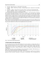
Fig. 3. PSD
P
+(f) parameterization of active power of a 750 kW wind turbine for wind
speeds around 6,7 m/s (average power 190 kW) computed from 13 minute data.
The signal in the time domain can be computed from the inverse Fourier transform:

*
2
0
() ( )
() () 2 ()cos 2 ()
jft
Pf P f
P t T P f e df T P f f t f df
π
πϕ
∞∞
−∞
=−

⎡
⎤
== +
⎢
⎥
⎣
⎦
∫∫


(2)
An analogue relation can be derived for reactive power and wind, both for continuous and
discrete time. Standard FFT algorithms use two sided spectra, with negative frequencies in
the last half of the output vector. Thus, calculus will be based on two-sided spectra unless
otherwise stated, as in (2). In real signals, the negative frequency components are the
complex conjugate of the positive one and a ½ scale factor may be applied to transform one
to two-sided magnitudes.
b) Spectral power balance in a wind farm
Fluctuations at the point of common coupling (PCC) of the wind farm can be obtained from
power balance equations for the average complex power of the wind farm.
Neglecting the increase in power losses in the grid due to fluctuating generation, the sum of
oscillating power from the turbines equals the farm output undulation. Therefore, the
complex sum of the frequency components of each turbine
()
turbine i
Pf

totals the
approximate farm output,
()

farm
Pf

:
From Turbine to Wind Farms - Technical Requirements and Spin-Off Products

110
()
111
() () () ()
turbines turbines turbines
i
NNN
j
f
farm
farm turbine i turbine i
iiturbinei
iii
turbine i
P
Pf Pf Pf Pfe
P
ϕ
ηη
===
∂
≅≈=
∂
∑∑∑



(3)
For usual wind farm configurations, total active losses at full power are less than 2% and
reactive losses are less than 20%, showing a quadratic behaviour with generation level (Mur-
Amada & Comech-Moreno, 2006). A small-signal model of power losses due to fluctuations
inside the wind farm can be derived (Kundur et al. 1994), but since they are expected to be
up to 2% of the fluctuation, the increase of power losses due to oscillations can be neglected
in the first instance. A small signal model can be used to take into account network losses
multiplying the turbine phasors in (3) by marginal efficiency factors
/
ifarmturbinei
PPη =∂ ∂
estimated from power flows with small variations from the mean values using
methodologies as the point-estimate method (Su, 2005; Stefopoulos et al., 2005). Typical
values of
i
η are about 98% for active power and about 85% for reactive power. In some
expressions of this chapter, the efficiency has been set to 100% for clarity in the formulas.
In some applications, we encounter a random signal that is composed of the sum of several
random sinusoidal signals, e.g., multipath fading in communication channels, clutter and
target cross section in radars, interference in communication systems, wave propagation in
random media and channels, laser speckle patterns and light scattering and summation of
random current harmonics such as the ones produced by high frequency power converters
of wind turbines (Baghzouz et al., 2002; Tentzerakis & Papathanassiou, 2007).
Any random sinusoidal signal can be considered as a random phasor, i.e., a vector with
random length and angle. In this way, the sum of random sinusoidal signals is transformed
into the sum of 2-D random vectors. So, irrespective of the type of application, we encounter
the following general mathematical problem: there are vectors with lengths
||

ii
P P=

and
angles ϕ
i
= ()
i
Arg P

, in polar coordinates, where P
i
and ϕ
i
are random variables, as in (3)
and Fig. 4. It is desired to obtain the probability density function (pdf) of the modulus and
argument of the resulting vector. A comprehensive literature survey on the sum of random
vectors can be obtained from (Abdi, 2000).


1
()
1
()·
jf
Pfe
ϕ
2
()
2

()·
jf
Pfe
ϕ
3
()
3
()·
jf
Pfe
ϕ
4
()
4
()·
jf
Pfe
ϕ
2wfπ=
[Im]Y
[Re]X

Fig. 4. Model of the phasor diagram of a park with four turbines with a fluctuation level
P
i
(f ) and random argument ϕ
i
(f ) revolving at frequency f.
Avera
g

e fasor modulus
Power Fluctuations in a Wind Farm Compared to a Single Turbine

111
The vector sum of the four phasor in Fig. 4 is another random phasor corresponding to the
farm phasor, provided the farm network losses are negligible. If some conditions are met,
then the farm phasor can be modelled as a complex normal variable. In that case, the phasor
amplitude has a Rayleigh distribution. The frequency f = 0 corresponds to the special case of
the average signal value during the sample.
c) One and two sided spectra notation
One or two sided spectra are consistent –provided all values refer exclusively either to one
or to two side spectra. Most differences do appear in integral or summation formulas – if
two-sided spectra is used, a factor 2 may appear in some formulas and the integration limits
may change from only positive frequencies to positive and negative frequencies.
One-sided quantities are noted in this chapter with a + in the superscript unless the
differentiation between one and two sided spectra is not meaningful. For example, the one-
sided stochastic spectral phasor density of the active power at frequency f is:

()Pf
+

=
()Pf

+
()Pf−

= 2
()Pf


(4)
In plain words, the one-sided density is twice the two-sided density. For convenience, most
formulas in this chapter are referred to two-sided values.
d) Case study
Fig. 5 to Fig 8 show the power fluctuations of a wind farm composed by 27 wind turbines of
600 kW with variable resistance induction generator from VESTAS (Mur-Amada, 2009). The
data-logger recorded signals either at a single turbine or at the substation. In either case,
wind speed from the meteorological mast of the wind farm was also recorded.
The record analyzed in this subsection corresponds to date 26/2/1999 and time 13:52:53 to
14:07:30 (about 14:37 minutes). The average blade frequency in the turbines was
f
blade
≈ 1,48
±0,03 Hz during the interval. The wind speed, measured in a meteorological mast at 40 m
above the surface with a propeller anemometer, was
U
wind
= 7,6 m/s ±2,0 m/s (expanded
uncertainty).
The oscillations due to rotor position in Fig. 5 are not evident since the total power is the
sum of the power from 26 unsynchronized wind turbines minus losses in the farm network.
Fig. 6 shows a rich dynamic behaviour of the active power output, where the modulation
and high frequency oscillations are superimposed to the fundamental oscillation.
3. Asymptotic properties of the wind farm spectrum
The fluctuations of a group of turbines can be divided into the correlated and the
uncorrelated components.
On the one hand, slow fluctuations (
f < 10
-3
Hz) are mainly due to meteorological dynamics

and they are widely correlated, both spatially and temporally. Slow fluctuations in power
output of nearby farms are quite correlated and wind forecast models try to predict them to
optimize power dispatch.
On the other hand, fast wind speed fluctuations are mainly due to turbulence and microsite
dynamics (Kaimal, 1978). They are local in time and space and they can affect turbine
control and cause flicker (Martins et al., 2006). Tower shadow is usually the most noticeable
fluctuation of a turbine output power. It has a definite frequency and, if the blades of all
turbines of an area became eventually synchronized, it could be a power quality issue.

From Turbine to Wind Farms - Technical Requirements and Spin-Off Products

112

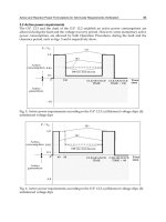
Fig. 5. Time series (from top to bottom) of the active power
P [MW] (in black), wind speed
U
wind
[m/s] at 40 m in the met mast (in red) and reactive power Q [MVAr] (in dashed green).


Fig. 6. Detail of the wind farm active power during 20 s at the wind farm.
The phase ϕ
i
(f) implies the use of a time reference. Since fluctuations are random events,
there is not an unequivocal time reference to be used as angle reference. Since fluctuations
can happen at any time with the same probability –there is no preferred angle ϕ
i
(f)–, the
phasor angles are random variables uniformly distributed in [-π,+π] (i.e., the system
exhibits circular symmetry and the stochastic process is cyclostationary). Therefore, the

relevant information contained in ϕ
i
(f) is the relative angle difference among the turbines of
the farm (Li et al., 2007) in the range [-π,+π], which is linked to the time lag among
fluctuations at the turbines.
The central limit for the sum of phasors is a fair approximation with 8 or more turbines and
Gaussian process properties are applicable. Therefore, the wind farm spectrum converges
asymptotically to a complex normal distribution, denoted by
()
0, ( )
Pfarm
Nfσ . In other
words,
Re[ ( )]
farm
Pf
+

and Im[ ( )]
farm
Pf
+

are independent random variables with normal
distribution.
Power Fluctuations in a Wind Farm Compared to a Single Turbine

113

Fig. 7.
PSD
P
+(f) parameterization of real power of a wind farm for wind speeds around
7,6 m/s (average power 3,6 MW) computed from data of Fig. 5.



Fig. 8. Contribution of each frequency to the variance of power computed from Fig. 5 (the
area bellow f·PSD
P
+(f) in semi-logarithmic axis is the variance of power).

()
() 0, ()
farm farm
Pf N fσ
+

∼ (5)
Thus, the one-sided amplitude density of fluctuations at frequency f from N turbines,
()
farm
Pf
+

, is a Rayleigh distribution of scale parameter ()
Pfarm
f
σ = |()|2/

farm
Pf π
+
〈〉

,
where angle brackets i denotes averaging. In other words, the mean of ()
farm
Pf
+

is
|()|
farm
Pf
+
〈〉

= /2π ()
Pfarm
f
σ where ()
Pfarm
f
σ is the RMS value of the phasor projection.
The RMS value of the phasor projection ()
Pfarm
f
σ is also related to the one and two sided
PSD of the active power:

From Turbine to Wind Farms - Technical Requirements and Spin-Off Products

114

()
Pfarm
f
σ =
2()
Pfarm
PSD f
=
()
Pfarm
PSD f
+
(6)
Put into words, the phasor density of the oscillation,
()
Pfarm
Pf
+

, has a Rayleigh
distribution of scale parameter
()
Pfarm
f
σ equal to the square root of the auto spectral
density (the equivalent is also hold for two-sided values). The mean phasor density

modulus is:

(())
|()| ()
2
Pfarm
Pfarm Pfarm
Rayleigh f
Pf f
σ
π
σ
+
〈〉=

(7)
For convenience, effective values are usually used instead of amplitude. The effective value
of a sinusoid (or its root mean square value, RMS for short) is the amplitude divided by √2.
Thus, the average quadratic value of the fluctuation of a wind farm at frequency
f is:

2
2
2
[()]
()/ 2 () /2 () ()
N
Pfarm Pfarm Pfarm Pfarm
Rayleigh f
Pf Pf fPSDf

σ
σ
++ +
===


(8)
If the active power of the turbine cluster is filtered with an ideal narrowband filter tuned at
frequency f and bandwidth Δf, then the average effective value of the filtered signal is
()
Pfarm
f
fσ Δ and the average amplitude of the oscillations is |()|·
farm
Pf f
+
〈〉Δ

=
() · /2
Pfarm
ffσπΔ
. The instantaneous value of the filtered signal
,,
()
Pfarm f f
Pt
Δ

is the

projection of the phasor
2
()·
jft
farm
Pfe f
π+
Δ

in the real axis. The instantaneous value of the
square of the filtered signal,
2
,,
()
farm f f
Pt
Δ
, is an exponential random variable of parameter
λ=
21
[()]
farm
f
fσ
−
Δ and its mean value is:

22
,,
() ( )

farm f f Pfarm
Exp distribution
Pt ffλσ
Δ
== Δ
(9)

For a continuous PSD, the expected variance of the instantaneous power output during a
time interval
T is the integral of ()
Pfarm
f
σ between Δf = 1/T and the grid frequency,
according to Parseval’s theorem (notice that the factor 1/2 must be changed into 2 if two-
sided phasors densities are used):

22 22
1/ 1/ 1/
11
() |()| |()| ()
22
grid grid grid
fff
farm farm farm farm
TTT
P t P f df P f df f dfσ
++
==〈〉=
∫∫∫



(10)

In fact, data is sampled and the expected variance of the wind farm power of duration T can
be computed through the discrete version of (10), where the frequency step is Δ
f = 1/T and
the time step is Δ
t= T/m:
111
22 22
111
11
() |()| |()| ()
22
mmm
farm farm farm Pfarm
kkk
Pt Pkff Pkff kffσ
−−−
++
===
=ΔΔ=〈Δ〉Δ=ΔΔ
∑∑∑

(11)
Power Fluctuations in a Wind Farm Compared to a Single Turbine

115
If a fast Fourier transform is used as a narrowband filter, an estimate of
2

()
Pfarm
f
σ for
f = k Δf is
{}
2
2·| ( )|
kfarm
f FFT P i tΔ〈 Δ 〉
. In fact, the factor 2
f
Δ may vary according to the
normalisation factor included in the
FFT, which depends on the software used. Usually,
some type of smoothing or averaging is applied to obtain a consistent estimate, as in Bartlett
or Welch methods (Press et al., 2007).
The distribution of
2
()
farm
Pt can be derived in the time or in the frequency domain. If the
process is normal, then the modulus and phase of
()
f
arm k
Pf
+

are not linearly correlated at

different frequencies
k
f
. Then
2
()
farm
Pt is the sum in (11) or the integration in (10) of
independent Exponential random variables that converges to a normal distribution with
mean
2
()
farm
Pt and standard deviation
2
2()
farm
Pt.
In farms with a few turbines, the signal can show a noticeable periodic fluctuation shape
and the auto spectral density
2
()
Pfarm
f
σ can be correlated at some frequencies. These
features can be discovered through the bispectrum analysis. In such cases,
2
()
farm
Pt can be

computed with the algorithm proposed in (Alouini et al., 2001).
4. Sum of partially correlated phasor densities of power from several turbines
4.1 Sum of fully correlated and fully uncorrelated spectral components
If turbine fluctuations at frequency
f of a wind farm with N turbines are completely
synchronized, all the phases have the same value ϕ
(f) and the modulus of fully correlated
fluctuations
,
|()|
icorr
Pf
+

sum arithmetically:

, , ,
11
| ( )| ( ) | ( )|
NN
farm corr i i corr i i corr
ii
P f Pf Pfηη
+++
==
==
∑∑

(12)
If there is no synchronization at all, the fluctuation angles ϕ

i
(f) at the turbines are
stochastically independent. Since
,
()
iuncorr
Pf


has a random argument, its sum across the
wind farm will partially cancel and inequality (13) holds true.

, , ,
11
|()| ()|()|
NN
farm uncorr i i uncorr i i uncorr
ii
P f Pf Pfηη
+++
==
=<
∑∑

(13)
This approach remarks that correlated fluctuations adds arithmetically and they can be an
issue for the network operation whereas uncorrelated fluctuations diminish in relative terms
when considering many turbines (even if they are very noticeable at turbine terminals).
A) Sum of uncorrelated fluctuations
The fluctuation of power output of the farm is the sum of contributions from many turbines

(3), which are mainly uncorrelated at frequencies higher than a tenth of Hertz.
The sum of
N
independent phasors of random angle of
N
equal turbines in the farm
converges asymptotically to a complex Gaussian distribution,
()
farm
Pf


~
[0, ( )]
Pfarm
Nfσ
,
of null mean and standard deviation ()
farm
fσ =
1
()Nfησ , where
1
()
f
σ is the mean RMS
fluctuation at a single turbine at frequency
f
and η is the average efficiency of the farm
network. To be precise, the variance

2
1
()
f
σ
is half the mean squared fluctuation amplitude
From Turbine to Wind Farms - Technical Requirements and Spin-Off Products

116
at frequency
f,
2
1
()
f
σ

=
2
1
2
()
turbine i
Pf


=
2

Re ( )

turbine i
Pf
⎡
⎤
⎢
⎥
⎣
⎦


=
2

Im ( )
turbine i
Pf
⎡
⎤
⎢
⎥
⎣
⎦


.
Therefore, the real and imaginary phasor components
Re[ ( )]
farm
Pf



and
Im[ ( )]
farm
Pf


are
independent real Gaussian random variables of standard deviation
()
Pfarm
f
σ
and null
mean since phasor argument is uniformly distributed in [–π,+π]. Moreover, the phasor
modulus
()
farm
Pf


has [()]
Pfarm
Rayleigh fσ distribution. The double-sided power spectrum
2
()
farm
Pf



is an
2
1
2
()
Pfarm
fExponential σλ
−
⎡
⎤
=
⎢
⎥
⎣
⎦
random vector of mean
2
()
farm
Pf



=
2
2()
Pfarm
f
σ
=

1
2
()
Pfarm
PSD f
(Cavers, 2003).
The estimate from the periodogram is the moving average of
N
aver.
exponential random
variables corresponding to adjacent frequencies in the power spectrum vector. The estimate
is a Gamma random variable. If the
PSD is sensibly constant on N
aver
Δf bandwidth, then the
PSD estimate has the same mean as the original PSD and the standard deviation is
.aver
N times smaller (i.e., the estimate has lower uncertainty at the cost of lower frequency
resolution).
4.2 Sum of partially linearly correlated spectral components
Inside a farm, the turbines usually exhibit a similar behaviour for a given frequency
f and
the PSD of each turbine is expected to be fairly similar. However, the phase differences
among turbines do vary with frequency. Slow meteorological variations affect all the
turbines with negligible time lag, compared to characteristic time frame of weather systems
(i.e., the phasors
()
turbine
Pf


have the same phase). Turbulences with scales significantly
smaller than the turbine distances have uncorrelated phases. Fluctuations due to rotor
positions also show uncorrelated phases provided turbines are not synchronized.

22 2
,,
() () ()
turbine turb corr turb uncorr
Pf P f P f
++ +
=+
(14)
If the number of turbines
N >4 and the correlation among turbines are linear, the central
limit is a good approximation. The correlated and uncorrelated components sum
quadratically and the following relation is applicable:

()
22
2
2
,,
() () ()
farm turb corr turb uncorr
Pf N P f NP fηη
+++
≈+


(15)

where N is the number of turbines in the farm (or in a group of close farms) and
η
is the
average efficiency of the farm network (typical values are about 98% for active power and
about 85% for reactive power). Since phasor densities sum quadratically, (14) and (15) are
concisely expressed in terms of the
PSD of correlated and uncorrelated components of
phasor density:

()
2
,,
() () · ()
farm turb corr turb uncorr
PSD f N PSD f N PSD fηη≈+
(16)

,,
() () ()
turb turb corr turb uncorr
PSD f PSD f PSD f=+
(17)
Power Fluctuations in a Wind Farm Compared to a Single Turbine

117
The correlated components of the fluctuations are the main source of fluctuation in large
clusters of turbines. The farm admittance
()Jf is the ratio of the mean fluctuation density of
the farm,

()
farm
Pf


, to the mean turbine fluctuation density, |()|
turbine
Pf
+
.
()Jf =
|()|
|()|
farm
turbine
Pf
Pf
+
+
≈
()
()
Pfarm
Pturbine
PSD f
PSD f
(18)
Note that the phase of the admittance
()Jf has been omitted since the phase lag between
the oscillations at the cluster and at a turbine depend on its position inside the cluster. The

admittance is analogous to the expected gain of the wind farm fluctuation respect the
turbine expected fluctuation at frequency
f (the ratio is referred to the mean values because
both signals are stochastic processes).
Since turbine clusters are not negatively correlated, the following inequality is valid:

()NJf Nηη11
(19)
The squared modulus of the admittance
()Jf is conveniently estimated from the PSD of the
turbine cluster and a representative turbine using the cross-correlation method and
discarding phase information (Schwab et al., 2006):

()
2
,,
2
() () ()
()
() () ()
Pfarm turb corr turb uncorr
Pturb turb turb
PSD f PSD f PSD f
Jf N N
PSD f PSD f PSD f
ηη== +
(20)
If the PSD of a representative turbine,
()
Pturb

PSD f
, and the PSD of the farm
()
Pfarm
PSD f

are available, the components
,
()
turb corr
PSD f and
,
()
turb uncorr
PSD f can be estimated from (16)
and (17) provided the behaviour of the turbines is similar.
At
f  0,01 Hz, fluctuations are mainly correlated due to slow weather dynamics,
,
()
turb uncorr
PSD f 
,
()
turb corr
PSD f , and the slow fluctuations scale proportionally
()
Pfarm
PSD f
≈

,
2
()()
turb corr
PSD fNη . At f > 0,01 Hz, individual fluctuations are statistically
independent,
,
()
turb uncorr
PSD f 
,
()
turb corr
PSD f , and fast fluctuations are partially attenuated,
()
Pfarm
PSD f
≈
,
()·
turb uncorr
PSD fNη .
An analogous procedure can be replicated to sum fluctuations of wind farms of a
geographical area, obtaining the correlated
,
()
farm corr
PSD f and uncorrelated
,
()

farm uncorr
PSD f
components. The main difference in the regional model –apart from the scattered spatial
region and the different turbine models– is that wind farms must be normalized and an
average farm model must be estimated for reference. Therefore, the average farm behaviour
is a weighted average of individual farms with lower characteristic frequencies (Norgaard &
Holttinen, 2004). Recall that if hourly or even slower fluctuations are studied, meteorological
dynamics are dominant and other approaches are more suitable.
4.3 Estimation of wind farm power admittance from turbine coherence
The admittance can be deducted from the farm power balance (3) if the coherence among
the turbine outputs is known. The system can be approximated by its second-order statistics
From Turbine to Wind Farms - Technical Requirements and Spin-Off Products

118
as a multivariate Gaussian process with spectral covariance matrix
()
P
f
Ξ . The elements of
()
P
f
Ξ are the complex squared coherence at frequency f and at turbines i and j, noted as
()
ij
f
γ

. The efficiency of the power flow from the turbine i to the farm output can be
expressed with the column vector

12
[ , , , ]
T
PN
ηηηη= , where
T
denotes transpose.
Therefore, the wind farm power admittance
()Jf is the sum of all the coherences,
multiplied by the efficiency of the power flow:

2'
11
() ( ) ()
NN
T
ijij P P P
ij
Jf f fηη γ η η
==
≈=Ξ
∑∑

(21)
The squared admittance for a wind farm with a grid layout of n
long
columns separated d
long
distance in the wind direction and n
lat

rows separated d
lat
distance perpendicular to the wind
U
wind
is:
12 1 2
2222 22
21 21
22
21
111 1
2( -) (-) + ( -
(
)
)
long long
lat lat
long lat lat long long
wind wind
nn
nn
ii j j
jjd f f A
Jf Cos Ex
ii d d
p
Ajj
UU
η

π
====
≈
−
⎡
⎤
⎡
⎤
⎢
⎥
⎢⎥
⎢
⎥
⎢⎥
⎢
⎥
⎢⎥
⎢
⎥
⎣
⎦
⎣
⎦
∑∑∑∑
(22)
The admittance computed for Horns Rev offshore wind farm (with a layout similar to Fig.
10) is plotted in Fig. 9. According to (Sørensen et al., 2008), it has 80 wind turbines disposed
in a grid of
n
lat

= 8 rows and n
long
= 10 columns separated by seven diameters in each
direction (
d
lat
= d
long
= 560 m), high efficiency (
η
≈ 100%), lateral coherence decay factor
A
lat
≈ U
wind
/(2 m/s), longitudinal coherence decay factor A
long
≈ 4, wind direction aligned
with the rows and
U
wind
≈ 10 m/s wind speed.
4.4 Estimation of wind farm power admittance from the wind coherence
The wind farm admittance ()Jf can be approximated from the equivalent farm wind
because the coherence of power and wind are similar (the transition frequency between
correlated and uncorrelated behaviour is about 10
-2
Hz for small wind farms). According to
(Mur-Amada, 2009), the equivalent wind can be roughly approximated by a multivariate

10 20 50 100 200 500 1000 2000
10
50
20
30
15
70
Frequency

cycles

day

Admittance

Fig. 9. Admittance for Horns Rev offshore wind farm for 10 m/s and wind direction aligned
with the turbine rows.
80η
80η
Power Fluctuations in a Wind Farm Compared to a Single Turbine

119
Gaussian process with spectral covariance matrix
()
Ueq
f
Ξ . Its elements are the complex
coherence of effective turbulence at frequency
f and at turbines i and j, denoted by
'

()
ij
f
γ

.
In this case, the column vector
'' '
12
[, , , ]
T
Ueq N
ηηηη= should be interpreted as the relative
sensitivity of the farm power respect the equivalent wind in each turbine. Therefore, the
wind farm power admittance
()Jf is the sum of the complex coherence of effective
quadratic turbulence among turbines:

2'''
11
() ( ) ()
NN
T
i j ij Ueq Ueq Ueq
ij
Jf f fηηγ η η
==
≈=Ξ
∑∑


(23)
For the rectangular region shown in Fig. 10, the admittance is:

()
{}
22
() 1 ( 1)Jf N N H fηη≈+−
(24)
where

,
,
2
()
()
(+2)

() Re
Ueq area
Ueq turbine
long
lat
wind wind
PSD f
PSD f
Ajaf
Abf
Hf g g
UU
π

⎡
⎛⎞⎤
⎛⎞
⎟
⎜
⎟
⎜
⎢
⎥
⎟
⎜
⎟
==
⎜
⎟
⎟
⎜
⎢
⎥
⎜
⎟
⎟
⎜
⎜
⎟
⎜
〈〉 〈〉
⎝⎠
⎝⎠
⎢

⎥
⎣
⎦
(25)

()
x2
21)x(/egxx
−
−+ += (26)
wind
U〈〉 is the mean wind during the sample, η is the average sensitivity of the power
respect the wind and
a and b are the dimensions of the wind farm according to Fig. 10. The
decay constants for lateral and longitudinal directions are,
A
long
and A
lat
, respectively. For
the Rutherford Appleton Laboratory, (Schlez & Infield, 1998) recommended
A
long
≈ (15±5)
σ
Uwind
/
wind
U
and A

lat
≈ (17,5±5) (m/s)
-1
σ
Uwind
, where σ
Uwind
is the standard deviation of
the wind speed in m/s. IEC 61400-1 recommends
A ≈ 12; Frandsen (Frandsen et al., 2007)
recommends
A ≈ 5 and Saranyasoontorn (Saranyasoontorn et al., 2004) recommends
A ≈ 9,7.
2
()Hf is the quadratic coherence between the equivalent wind of the farm, relative to the
turbine.
()Hf measures the correlation of the phase difference between the equivalent wind
of the farm relative to the turbine at frequency f. If
()Hf is unity, the turbine phasors have


β=0
b
wind
direction
a

Fig. 10. Wind farm dimensions for the case of frontal wind direction.
From Turbine to Wind Farms - Technical Requirements and Spin-Off Products

120
the same angle and the turbine fluctuations are synchronized at that frequency. If
()Hf is
zero, the phasors have uncorrelated arguments and hence, the turbine fluctuations are
stochastically uncorrelated at that frequency. Hence,
()Hf is the correlation level at
frequency
f of the fluctuations among the turbines, measured from 0 to 1.
The transition frequency from correlated to uncorrelated fluctuations is obtained solving
2
()Hf
=1/4. Thus, the cut-off frequency of narrow wind farms with a « b is:

,
6.83
w
cut l
ind
at
lat
f
U
bA
〈〉
= (27)
In the Rutherford Appleton Laboratory (RAL),
A
lat
≈ (17,5±5)(m/s)
-1

σ
Uwind
and hence f
cut,lat
≈
(0,42±0,12)
wind
U〈〉/ (σ
Uwind
b). A typical value of the turbulence intensity σ
Uwind
/
wind
U〈〉 is
around 0,12 and for such value
f
cut,lat
~ (3.5±1)/b, where b is the lateral dimension of the area
in meters. For a narrow farm of
b = 3 km, the cut-off frequency is in the order of 1,16 mHz.
In Horns Rev wind farm,
A
lat
=
wind
U
/(2 m/s) and hence f
cut,lat
≈ 13,66/b, where b is a
constant expressed in meters. For a wind farm of

b = 3 km, the cut-off frequency is in the
order of 4,5 mHz (about four times the estimation from RAL).
In RAL,
A
long
≈ (15±5) σ
Uwind
/
wind
U
. A typical value of the turbulence intensity σ
Uwind
/
wind
U〈〉 is around 0,12 and for such value A
l
ong
≈ (1,8±0,6).

,
1,8 1 .8
1,1839 0.6577
long long
win
cut long
AA
long
dwind
UU
f

aA a
=
〈〉 〈
==
〉
∼
(28)
For a significative wind speed of
wind
U〈〉~10 m/s and a wind farm of a = 3 km longitudinal
dimension, the cut-off frequency is in the order of 2,19 mHz.
In the Høvsøre wind farm,
A
long
= 4 (about twice the value from RAL). The cut-off frequency
of a longitudinal area with
A
long
around 4 (dashed gray line in Fig. 11) is:

,
44
2.7217 0.6804
long long
wi
cut long
AA
lon
n
g

nd wi d
U
f
a
U
aA
=
〈〉 〈
==
〉
∼
(29)
For a significative wind speed of
wind
U〈〉~ 10 m/s and a wind farm of a = 3 km
longitudinal dimension, the cut-off frequency is in the order of 2,26 mHz.
In accordance with experimental measurements, turbulence fluctuations quicker than a few
minutes are notably smoothed in the wind farm output. This relation is proportional to the
dimensions of the area where the wind turbines are sited. That is, if the dimensions of the
zone are doubled, the area is four times the original region and the cut-off frequencies are
halved. In other words, the smoothing of the aggregated wind is proportional to the longitudinal
and lateral lengths (and thus, related to the square root of the area if zone shape is
maintained).
In sum, the lateral cut-off frequency is inversely proportional to the site parameters
A
lat
and
the longitudinal cut-off frequency is only slightly dependent on A
long.
Note that the

longitudinal cut-off frequency show closer agreement for Høvsøre and RAL since it is
dominated by frozen turbulence hypothesis.
Power Fluctuations in a Wind Farm Compared to a Single Turbine

121

Fig. 11. Normalized ratio H
2
(f) for transversal a « b (solid thick black line) and longitudinal a
» b areas (dashed dark gray line for
A
long
= 4, long dashed light gray line for A
long
= 1,8).
Horizontal axis is expressed in either longitudinal or lateral adimensional frequency
a A
long
f /〈U
wind
〉 or b A
lat
f /〈U
wind
〉.
However, if transversal or longitudinal smoothing dominates, then the cut-off frequency is
approximately the minimum of
,cut lat
f
and

,cut long
f
. The system behaves as a first order
system at frequencies above both cut-off frequencies, and similar to a ½ order system
between
,cut lat
f
and
,cut long
f
.
5. Case study: comparison of PSD of a wind farm with respect to one of its
turbines during 12 minutes
A literature review on experimental data of power output PSD from wind turbines or wind
farms can be found in (Mur-Amada & Bayod-Rujula, 2007), with a parameterization and
analysis of the data from very different locations. (Apt, 2007) shows an interesting
comparison of the spectrum of the wind power from a wide area.
In this sub-section, the analysis of a case based on (Mur-Amada, 2009) is presented. The
similarity of the
PSD at one turbine and at the overall output of a wind farm of 18 turbines
is shown. If the fluctuations at every turbine are independent (i.e. the turbines behaves
independently from each other), then the
PSD of the wind farm is approximately the PSD of
each turbine multiplied by the number of turbines and by the power flow efficiency.
Each turbine experiments different turbulence levels and wind averages, so a representative
turbine should be selected. The time lag between the variations measured in the farm and in
the turbine depends on the farm layout. The phase information has been discarded because
the phase of ergodic stochastic processes do not contain statistical information.
Fig. 12 shows the power output of the wind farm and the scalled output of one turbine.
Since the measured turbine is more exposed to the wind than others turbines, the ratio of the

average power of the turbine to the farm is 14 (less than 18, the number of turbines in the
farm). There is a clear reduction of the relative variability in the farm output and some slow
From Turbine to Wind Farms - Technical Requirements and Spin-Off Products

122
oscillations between the turbine and the farm seem to be delayed. In fact, this section will
show that the ratio of the fluctuations is about √18 because the measured fluctuations are
mainly uncorrelated, the duration of the sample is relatively short (less than 12 minutes) and
the wind does not show a noticeable trend during the sample.
If the turbines behave independently from each other and they are similar, then the
PSD of
the wind farm is the
PSD of one turbine times the number of turbines in the farm and times
a power efficiency factor. To test this hypothesis, the farm
PSD is shown in solid black and
the turbine
PSD times 18 is in dashed green in Fig. 13, with good agreement.


Fig. 12. Power output of the wind farm (in solid black) and the power of the turbine times 14.
Fig. 13 shows that the farm
PSD
P
+
(f) and the scaled turbine PSD
P
+
(f) agree notably, showing
that fluctuations up to 10
-2

Hz are almost uncorrelated (frequency bellow 10
-2
Hz is shown in
the figure, but its value is biased by the window applied in the FFT and the relative short
duration of the sample). However, the wind farm
PSD is a bit lower than 18 times the
turbine PSD, specially at the peaks and at f > 2f
blade
(f
blade
is the frequency of a blade crossing
the turbine tower, about 1,54 Hz in this sample). On the one hand, this turbine experiences
more cyclic oscillations, partly due to a misalignment of the rotor bigger than the farm
average. On the other hand, this turbine produced an average of 1/14
th
of the wind farm
power on the series #1 (see Fig. 12). This explain that PSD at f > 2f
blade
is primarily
proportional to power output ratio (the farm
PSD is 14 times the turbine PSD).
The real power admittance is shown in Fig. 14. The admittance is the ratio of the farm
spectrum to the turbine spectrum of real power and it can be estimated as the square root of
the
PSD ratios. The level √18 has been added in dash-dotted red line to compare with the
theoretical value of uncorrelated fluctuations.
In general terms, the assumption of uncorrelated fluctuations at frequencies higher than
10
-2
Hz is valid: the admittance is approximately √18, the square root of the number of

turbines in the farm. At f > 2f
blade
, the admittance is more similar to √14 (the square root of
the farm power divided by the turbine power). At f < 0,02 Hz, the admittance starts drifting
from √18, indicating that oscillations at very low frequency are somewhat correlated.
Power Fluctuations in a Wind Farm Compared to a Single Turbine

123

Fig. 13. PSD
Pfarm
+
(f) of a wind farm (in solid black) and PSD
Pturbine
+
(f) of one of its 648 kW
turbines times 18 (in dashed green), for time series #1.
There is a peak in Fig. 14 at 2 Hz < f < 2,5 Hz. The analyzed turbine may have comparative
less fluctuations in such range than the other turbines in the farm (the measured turbine
may have better adjusted rotor and blades, while others turbines may suffer from more
vibration effects). But other feasible reason is a higher correlation degree between the
turbines at such frequency band, probably induced by turbine control or voltage variations.


Fig. 14. Admittance of the active power (ratio of the farm
PSD to the turbine PSD).
In short, real power oscillations quicker than one minute can be considered independent
among turbines of a wind farm because the PSD due to fast turbulence and rotational effects
scales proportionally to the number of turbines.