Process Engineering for Pollution Control and Waste Minimization_6 ppt

∆G = RT ln
ƒ
2
ƒ
1
(real gas) (78)
Here, ƒ
1
is the fugacity at pressure P
1
. The fugacity may be considered as an
adjusted pressure. It is defined so as to coincide with the pressure at low densities:
lim
P→0
ƒ
P
= 1 (79)
The ratio of fugacity to pressure is called the fugacity coefficient, φ. Thus, the
previous equation may be written
ϕ≡
ƒ
P
⇒
lim
P→0
ϕ= 1 (80)
5.4 Chemical Potential
Consider a solution consisting of n species A, B, . . . . The Gibbs free energy of
the solution is given by
G =
∑

k=1
n
N
k
µ
k
(81)
where µ
k
is the chemical potential of species k, defined by
µ
k
=



∂G
∂N
k



T,P,N
j≠k
(82)
5.5 Fugacity and Activity
The chemical potential is generally a function of temperature, pressure, and
composition. It is common practice to write
µ
A

=µ˚
A
(T)+RT ln a
A
(83)
where µ˚
A
(T) is the standard chemical potential and a
A
is the activity of species
A. The activity is defined as the ratio of the fugacity ƒ
A
to a standard-state
fugacity ƒ˚
A
:
a
A
=
ƒ
A
ƒ˚
A
(84)
Activities and standard states are discussed in greater detail in many texts on
chemical thermodynamics (11,12).
Copyright 2002 by Marcel Dekker, Inc. All Rights Reserved.
5.6 Phase Equilibrium
Consider a multicomponent system that separates into two or more phases
(denoted I, II, . . .). The criteria for phase equilibrium are

T
I
= T
II
= . . . (thermal equilibrium) (85)
P
I
= P
II
= . . . (mechanical equilibrium) (86)
(µ
A
)
I
=(µ
A
)
II
= . . . (equilibrium for species A) (87)
(µ
B
)
I
=(µ
B
)
II
= . . . (equilibrium for species B) (88)
.
.

.
5.7 Reaction Equilibrium
Consider a reaction
aA + bB + . . . = . . . + xX + zZ
which, as before, can be expressed in the shorthand notation
0 =
∑
k=1
n
ν
k
I
k
The criterion for chemical reaction equilibrium is
∆G =
∑
k=1
n
ν
k
µ
k
= 0 (89)
Reaction equilibrium may also be expressed in terms of the standard Gibbs
free-energy change:
∆G
0
= RT ln K
a
(90)

Here, K
a
is the equilibrium constant, defined by
K
a
=
∏
k=1
n
a
k
ν
k
(91)
6 ENGINEERING FLUID MECHANICS
Fluid mechanics deals with the flow of liquids and gases. For most engineering
applications, a macroscopic approach is usually taken.
Copyright 2002 by Marcel Dekker, Inc. All Rights Reserved.
6.1 Engineering Bernoulli Equation
Most engineering problems in fluid mechanics can be solved using the engineer-
ing Bernoulli equation, also called the mechanical energy balance. It can be
derived from the macroscopic energy balance (see Ref. 13), subject to the
following restrictions: (a) the system is at steady state; (b) the system has a single
fluid intake and a single outlet; (c) gravity is the sole body force, with constant
|g|; (d) the flow is incompressible; (e) the system may include one or more pumps
or turbines. Under these conditions, the macroscopic energy balance becomes
∆




P
ρ
+ |g|z +
α
2
〈ν〉
2



=
W
⋅
s
m
⋅
−
F
⋅
m
⋅
(92)
where
P = the fluid pressure
〈ν〉 = the velocity averaged over the cross section of the pipe or conduit
α= average velocity correction factor (2.0 for laminar flow and 1.07 for
turbulent flow)
W
⋅
2

= rate of work done by pumps or turbines (positive for pumps,
negative for turbines)
F
⋅
= frictional loss rate
Dividing by the acceleration of gravity |g| yields the so-called head form of the
Bernoulli equation:
∆



P
ρ|g|
+ z +
α
2|g|
〈ν〉
2



=
W
⋅
s
m
⋅
|g|
−
F

⋅

m
⋅
|g|
(93)
Each of the terms in this equation has the dimensions of length.
6.2 Fluid Friction in Pipes and Conduits
The frictional loss rate F
⋅
equals the rate at which useful mechanical energy is
converted to thermal energy by friction. It is usually computed from an equation
of the form
F
⋅
m
⋅
= 4ƒ



L
D



〈ν〉
2
2
(94)

where ƒ is the Fanning friction factor.* In general, the friction factor is a function
*This is not the only friction factor in widespread use. Some authors prefer the Darcy-Wiessbach
friction factor, ƒ
DW
= 4ƒ.
Copyright 2002 by Marcel Dekker, Inc. All Rights Reserved.
of the pipe diameter D, the surface roughness ε, and the Reynolds number Re,
the latter being defined as
Re =
ρD|ν|
µ
(95)
where µ is the fluid viscosity.
In the laminar-flow regime, ƒ = 16/Re. For turbulent flows, a number of
charts, graphs, and equations are available to compute the friction factor. The
Colebrook equation has traditionally been used, although it requires a trial-and-
error solution to find ƒ:
1
√ƒ
=−4 log



ε/D
3.7
+
1.255
Re√ƒ




(96)
Wood’s approximation (Ref. 13) gives ƒ directly, without a trial-and-error
procedure:
ƒ = a + b Re
−c
(97)
where
a = 0.0235



ε
D



0.225
+ 0.1325



ε
D



(98)
b = 22




ε
D



0.44
(99)
c = 1.62



ε
D



0.134
(100)
The relations presented in this section were developed for cylindrical pipes or
tubes; however, the same equations may be used for noncylindrical ducts if the
pipe diameter D is replaced in Eqs. (94–100) by the hydraulic diameter D
H
:
D
H
= 4
volume of fluid
area wetted by fluid

(101)
6.3 Minor Losses
The relations developed in the previous section apply only to straight pipes or
conduits. Most pipelines, however, include bends, valves, and other fittings which
create additional frictional losses. These additional losses are often called “minor
losses,” although they may actually exceed the friction caused by the pipe itself.
There are two common ways to account for minor losses. One is to define
an equivalent length L
eq
which equals the length of straight pipe that would give
the same frictional loss as the valve or fitting in question. The total equivalent
Copyright 2002 by Marcel Dekker, Inc. All Rights Reserved.
length L
total
is the sum of the true length of the pipe and the individual equivalent
lengths of the valves and fitting:
L
total
= L
pipe
+
∑
fitting i
(L
eq
)
i
(102)
The total equivalent length L
total

is used in Eq. (94) in place of L to compute the
total frictional losses.
The second common approach to computing minor losses relies on the
concept of a loss coefficient K
L
, defined for each type of valve or fitting according
to the equation
F
⋅
m
⋅
= K
L
〈ν〉
2
2
(103)
A comprehensive listing of typical equivalent lengths and loss coefficients is
published by the Crane Company (14).
6.4 Fluid Friction in Porous Media
A porous medium is a solid material containing voids through which fluids may
flow. The most important single parameter used to described porous media is the
porosity or void fraction ε:
ε=
void volume
bulk volume
=
V
voids
V

voids
+ V
solid
(104)
Fluid friction in a porous medium of thickness L is usually described by Darcy’s law:
F
⋅
m
⋅
=
µ
ρ
L
k
〈ν〉 (105)
where k is a material property called the permeability.
REFERENCES
1. R. B. Bird, W. E. Stewart, and E. N. Lightfoot, Transport Phenomena. New York:
Wiley, 1960.
2. M. M. Denn, Process Fluid Mechanics. Englewood Cliffs, NJ: Prentice-Hall, 1980.
3. R. W. Fahien, Fundamentals of Transport Phenomena. New York: McGraw-Hill,
1983.
4. W. M. Deen, Analysis of Transport Phenomena. New York: Oxford University Press,
1998.
5. E. L. Cussler, Diffusion Mass Transfer in Fluid Systems, 2nd ed. Cambridge, U.K.:
Cambridge University Press, 1997.
Copyright 2002 by Marcel Dekker, Inc. All Rights Reserved.
6. O. Levenspiel, Chemical Reaction Engineering, 2nd ed. New York: Wiley, 1972.
7. H. S. Fogler, Elements of Chemical Reaction Engineering. Englewood Cliffs, NJ:
PTR Prentice-Hall, 1992.

8. L. D. Schmidt, The Engineering of Chemical Reactions. New York: Oxford Univer-
sity Press, 1998.
9. F. P. Incropera and D. P. DeWitt, Fundamentals of Heat and Mass Transfer, 3rd ed.
New York: Wiley, 1990.
10. D. R. Lide (ed.), CRC Handbook of Chemistry and Physics, 80th ed. Cleveland, OH:
CRC Press, 1999.
11. I. M. Klotz and R. M. Rosenberg. Chemical Thermodynamics: Basic Theory and
Methods, 3rd ed. Menlo Park, CA: W. A. Benjamin, 1972.
12. K. Denbigh, The Principles of Chemical Equilibrium, 3rd ed. Cambridge, U.K.:
Cambridge University Press, 1971.
13. N. De Nevers, Fluid Mechanics for Chemical Engineers, 2nd ed. New York:
McGraw-Hill, 1991.
14. Flow of Fluids Through Valves, Fittings, and Pipe, Crane Technical Paper 410.
Chicago: The Crane Company, 1988.
Copyright 2002 by Marcel Dekker, Inc. All Rights Reserved.
10
Biotechnology Principles
Teresa J. Cutright
The University of Akron, Akron, Ohio
1 INTRODUCTION
As mentioned throughout this text, waste minimization encompasses recycling/
reuse, waste reduction (material substitution, process changes, good housekeep-
ing, etc.), and waste treatment on-site (1,2). Biotechnology has a direct impact
on, and applicability to, an engineer’s ability to achieve waste minimization goals.
It has had demonstrated success with recycling programs via the generation of
biogas as an alternative fuel. Bioremediation approaches have also been used for:
point source reduction via biopolishing (3) and individual stream treatment (4);
by-product utilization (5); material substitution (6); facilitation of new enzy-
matic/metabolic pathways to produce “cleaner” organic substances (7); and
end-of-pipe treatments (8–10). This chapter will highlight a few of the biotech-

nology approaches to waste minimization.
When utilizing any biotechnology, it is important to remember that the
primary function of a microorganism is not to destroy man’s unwanted contami-
nants. Instead, a microbe must reproduce itself and maintain its cellular functions.
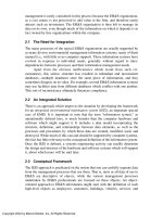
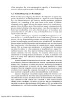
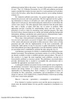
To that end, as shown in Figure 1, every microorganism must: (a) protect itself
from the environment, (b) secure nutrients (catabolism), (c) produce energy in a
usable form (catabolism), (d) convert nutrients/food into cellular material (anab-
olism); (e) discard unnecessary waste products, and (f) replication genetic infor-
Copyright 2002 by Marcel Dekker, Inc. All Rights Reserved.
FIGURE 1 Overview of general cellular functions applicable to all living cells.
Copyright 2002 by Marcel Dekker, Inc. All Rights Reserved.
mation. It is an added benefit to mankind that the result from the microbial
metabolism of substrates (i.e., step d), that the unwanted contaminants are
degraded. Once it was realized that microorganisms could degrade unwanted
contaminants, engineers started to manipulate the surrounding environment to
ensure that the microbes would thrive and utilize the contaminant as the substrate.
Engineers currently use microorganisms to treat drinking water, municipal
wastewater, and various industrial effluents. Usually the chemical and petrochem-
ical industry is considered the only “real” contributor to industrial effluent (11).
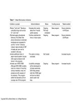
However, as shown in Table 1, more than just the chemical industry utilizes
microorganisms for the treatment of waste on-site.
Regardless of whether the microorganisms are being used for cleaning
drinking water, or municipal or industrial wastewaters; for end-of-pipe treatment
at contaminated sites; or for waste minimization applications, certain key aspects
apply (75). The following sections will outline the key aspects applicable to
any biological treatment, provide a brief description and design criteria for
the common waste minimization technologies, as well as highlight a few of the
TABLE 1 Some of the Industries that Utilize
Biological Treatment for the Reduction of
Waste

Industry References
Coal processing 12–14
Cosmetics 15,16
Dyes 16–20
Fertilizer plants 21,22
Food 23,24
Citric acid 23,24
Dairy 25–30
Poultry 31–34
Slaughterhouses 22,35,36
Vegetables 37,38
Heavy metals processing 13,39–45
Oil processing and refineries 46–49
Paint 50–53
Paper 6,21,22,54–57
Pesticides 13,18,58–60
Pharmaceutical 61–66
Printing 19,20,67,68
Soap 46,69
Tannery 22,70,71
Textiles 3,18,72–74
Copyright 2002 by Marcel Dekker, Inc. All Rights Reserved.
innovative of bioprocesses that enable the selective removal of unwanted chem-
icals in product streams.
2 KEY ELEMENTS ESSENTIAL TO ALL BIOLOGICAL
TREATMENT METHODS
Several basic biological requirements are essential for any biological treatment
process to be successful. They are based on the principles required to support all
ecosystems and include the presence of: appropriate microbes for degrading the
contaminant(s), substrate for carbon and energy source, required terminal electron

acceptor (TEA), inducer to facilitate enzyme synthesis, nutrients for supporting
microbial growth, microbes to degrade metabolic byproducts, environmental
conditions to minimize growth of competitive organisms (76–78). These factors
will be discussed below.
2.1 Adequate Microbial Population
The primary requirement for any successful biological treatment or waste mini-
mization strategy is the presence of an adequate microbial population. Luckily for
environmental engineers, Mother Nature has supplied a wide variety of microbes
to select from and to cultivate. The organisms are subdivided into different
categories based on their metabolic capabilities and/or requirements. Table 2
contains the classifications based on the microbial carbon source, energy source,
and respiration mode. If a contaminant can only be degraded in the presence of
another organic material that serves as the primary electron source, then co-
metabolism is occurring. If the interaction of the two organisms is nonobligatory,
then it is a synergistic relationship. Mutalism occurs if the interaction is beneficial
yet obligatory. Since microbes are very versatile, it is important to remember that
they may belong to more than category.
The microbe’s versatility may also enable it to treat more than one par-
ticular type of contaminant. As shown in Table 3, different species of Pseudo-
monas have demonstrated success at reducing agricultural, heavy metal, food,
and solvent wastes. In each instance, the primary requirement for successful
treatment is the presence of an adequate population. Researchers have deter-
mined that a microbial count of 10
3
–10
8
cfu/liter, 10
4
–10
7

cfu/g would be
adequate for groundwater and soil applications, respectively (77,79–81). There-
fore, to ensure a successful biological treatment for waste minimization, a
minimum of 10
8
cfu/liter would be recommended. If the contaminant concen-
tration or toxicity increases, the microbial population will have to increase as
well. If the increase in biomass concentration does not result in the desired
treatment efficiency, the microbes being utilized may have to be changed to
another source.
Copyright 2002 by Marcel Dekker, Inc. All Rights Reserved.
The species indigenous to a natural environment contain several different
microbes living together (i.e., mixed population). Therefore, it is reasonable to
presume that it is highly unlikely that one bacterial strain will be successful for a
complete waste minimization scheme. Table 3 includes bacteria that have been
successful at degrading the parent compound of the specified waste. Most of the
references did not report the achievement of complete mineralization (conversion
of contaminant into CO
2
, biomass, H
2
O, and salts). Complete mineralization
would require the use of a microbial consortium. A consortium is more than a
simple group of bacteria that can grow together. The overall net effect of the
consortium is greater than what the individual microbes can accomplish on its
own. Consortiums facilitate the degradation sequence where one microbe de-
TABLE 2 Microbial Classification Based on Growth Requirements: Carbon
and Energy Source, Respiration Mode
Term Definition
Prototrophs Most self-sufficient. Can synthesize all

required growth compounds given
CO
2
or a single organic compound.
Auxotrophs Cannot synthesize all compounds
required for growth.
Carbon source:
Autotrophs C source from CO
2
. Ex: algae, photosyn-
thetic bacteria.
Heterotrophs C obtained from reduced form of
organic compound.
Methanotrophs, methanogens C and energy source from methane.
Energy source:
Phototroph Derive energy from light (i.e., algae).
Chemotroph Derive energy from chemical oxidation.
Organotrophs Energy from oxidation of organic
chemicals.
Lithotrophs Energy from oxidation of inorganic
chemicals.
TEA:
Aerobe Require oxygen source for growth.
Anaerobe (oligate) Cannot grow in the presence of oxygen.
Obtain TEA from different source.
Facultative anaerobe Can utilize O
2
if present; however prefer-
able growth in absence of O
2

via differ-
ent TEA.
Fermentation TEA obtained from organic compound.
Copyright 2002 by Marcel Dekker, Inc. All Rights Reserved.
TABLE 3 Select Microbial Genus with Demonstrated Success for
Treating Industrial Contaminants Based on Waste Classification
Waste type Microbial genus
Aliphatics Achromobacter Micrococcus
Acinetobacter Mycobacterium
Arthrobacter Pseuodmonas
Bacillus Vibrio
Flavobacterium
Agricultural (pesticides, Achromobacter Flavobacterium
herbicides) Alcaligenes Methylomonas
Arthrobacter Penicillium*
Athiorocaceae Pseudomonas
Corneybacterium* Zylerion*
Dyes Aeromonas Phaneorchaete*
Micrococcus Shigella
Klebsiella Trametes*
Pseudomonas
Food, dairy, slaughter Acinetobacter Nitrosomonas
Arthrobacter Pseudomonas
Bacillus Rhodococcus
Brevibacterium Vibrio
Metals Aeromonas Pseudomonas
Alteromonas Saccharomyces†
Bacillus
Enterobacter
Pulp and paper Arthrobacter Talaromyces*

Eisenia Trichoderma*
Chromobacter Xanthomonas
Sporotrichum*
Solvents Alcaligenes Nitrosomonas
Citrobacter Nocardia
Desulfomonite Pseudomonas
Enterobacter Rhodococcus
Morganeela Xanthobacter
Mycobacterium
*Fungi; †yeast.
Copyright 2002 by Marcel Dekker, Inc. All Rights Reserved.
grades the metabolites of the first. The number and types of microbes required
for a successful consortium depends on the contaminant classification, complex-
ity, and concentration.
Natural mixed populations (i.e., consortiums) can be viewed as an interac-
tive community that require each individual presence in order to thrive. When
unmanipulated, the mixed population will contain one or two species that
dominate the culture. These species are the most adaptable to the surrounding
environment, have the most efficient energy utilization, and often facilitate the
first step in the metabolic pathway. As time progress, the population may shift to
one in which a different species dominates to continue the metabolic pathway or
adjust for changes in substrate, nutrients, or terminal electron acceptor (82–84).
The microbes used for waste minimization applications have three basic
modes of growth: attached (fixed), suspended, or free growth. Attached growth
is similar to the biofilms used in wastewater treatment (trickling filters) and air
emissions. Bioflims are surface aggregates composed of layers of bacteria that
are embedded in a polysaccharide matrix. Biofilms differ from suspended growth
in that they are fixed in a stationary place. Suspended growth systems (i.e.,
activated sludge) still have the bacteria attached to a surface, but the surface is
freely moving within the reactor. Free growth systems are similar to slurry

treatments where the bacteria can sorb and desorb from a surface.
2.2 Terminal Electron Acceptor
Without an adequate supply or specific type of TEA, biological treatment will
fail. Table 4 includes the primary electron acceptors used. Aerobic microbes
utilize O
2
as the TEA. For strict aerobes, the oxygen source is typically obtained
from air or H
2
O
2
. Incorporation of alternative TEA sources provide another name
to identify the respiration–microbe interaction. For instance, denitrifying bacteria
utilize nitrate (NO
3
−
→ NO
2
−
→ N
2
) as the TEA. Nitrobacter sp. is one of the
microbes capable of nitrification, the conversion of NH
3
-N to nitrates and
nitrates. Sulfate reducers, such as Desulfovibrio, utilize SO
4
2– and generate
TABLE 4 Typical TEAs and Their Associated Respiration Modes
TEA Form Mode

Oxygen O
2
Aerobic
Nitrate NO
3
Anaerobic
Sulfate SO
4
Anaerobic
Carbon dioxide CO
2
Methane fermentation
Organic compound Various Aerobic, anaerobic, fermentation
Copyright 2002 by Marcel Dekker, Inc. All Rights Reserved.
S
2–
(85). Methanogens require CO
2
as the TEA. Various bacteria can obtain the
TEA from organic compounds.
The specific type of electron acceptor will dictate the metabolism mode,
and thus the subsequent degradation reactions. Therefore the combination of
microbes and TEAs utilized will enable a specific degradation pathway to be
followed to facilitate cometabolism, prevent accumulation of toxic intermediates,
etc. (86,87).
2.3 Nutrients
The nutrient requirements for microbes are approximately the same as the
composition of their cells (76,88). The exception to this is carbon, which is
sometimes needed at higher quantities and can be supplied by the contaminant
for heterotrophic microorganisms. There are three categories of nutrients based

on the quantity and essential need for them by the microorganism: macro, micro,
and trace nutrients (89,90). For example, the macronutrients carbon, nitrogen, and
phosphorus are known to comprise 50%, 14%, and 3% dry weight, respectively,
of a characteristic microbial cell. Sulfur, calcium, and magnesium, which are
micronutrients, comprise only 1%, 0.5%, and 0.5%, respectively of the cells dry
weight (75,91,92). Trace nutrients, which are found in the least quantity, are not
required by all organisms. The most common trace elements are iron, manganese,
cobalt, copper, and zinc. Based on this approach, the optimal C:N:P mole ratio
recommended for bioremediation applications is 100:10:1 (77,93,94). For exam-
ple, 150 mg of nitrogen and 30 mg of phosphorous would be required to degrade
1 g of a theoretical hydrocarbon into cellular material. If the carbon source were
easily and rapidly converted into carbon dioxide, then more carbon would be
required in order to sustain microbes. For this reason, an additional carbon
supplement may need to be supplied to facilitate the degradation of the contam-
inant depending on the microbe–contaminant interaction. The limits of the carbon
(substrate) concentration will dictate the source and concentration of supplemen-
tal carbon and nutrients that are required (95).
Nitrogen is the nutrient most commonly added at bioremediation projects. It is
primarily used for cellular growth (NH
4
+
or NO
3
−
) for the synthesis of cellular
proteins and cell-wall components. It can also be used as an alternative electron
acceptor (NO
3
−
). It is commonly added as urea or as ammonium chloride but may

also be supplied as any ammonia salt or ammonium nitrate (92). All of these forms
are readily assimilated in bacterial metabolism. However, if an ammonium ion is used
to supply nitrogen, an increased oxygen demand on the surrounding system will be
created facilitating the need for additional TEA supplements (96).
Phosphorus is the second most commonly added nutrient in bioremediation
and is supplied to serve as a source for cellular growth. Often the ability of the
microbes to secure the required phosphorous levels depends on the correct
Copyright 2002 by Marcel Dekker, Inc. All Rights Reserved.
nitrogen level to be already in place (97). Phosphorus may be added as potassium
phosphate, sodium phosphate, or orthophosphoric and polyphosphate salts. Potas-
sium phosphate (mono- and di-basic) can also serve as a buffering agent to control
pH. However, there are also cautions regarding the addition of a phosphorus
source. The addition of potassium phosphate may accelerate the cleavage of the
hydrogen peroxide added as an oxygen source. If the hydrogen peroxide cleaves
too quickly, the oxygen source may be depleted before it reaches the contami-
nated zone. The maximum orthophosphate addition to provide microbial nutrients
while avoiding significant precipitation, peroxide cleavage, or toxicity in most
environments is 10 mg/liter (81).
Currently, there are no specific methods for predetermining the exact
nutrient sources to utilize for a given situation or the role they will play. The
specific ratio will depend on the chemicals to be treated, the microbes to be
utilized, and the presence of inorganic nutrients already in the waste stream (98).
The presence of a limiting nutrient will greatly affect the extent of remedial
treatment. Therefore, researchers have conducted studies to determine some
generalizations based on the type of microbe incorporated. For instance, nitrogen
is required in smaller quantities when fungi are utilized. Magnesium is required
in greater concentrations for photosynthetic bacteria. For aerobic cultures, iron is
necessary in higher quantities than their anaerobic counterparts. Even with these
generalizations, it is always a good idea to conduct a quick feasibility experiment
to determine the exact nutrients required (77). This is particularly true for

biological waste minimization processes with “exotic” chemicals, such as syn-
thetic polymers, pesticides, and pharmaceuticals.
2.4 Environmental Conditions
There are several other environmental conditions that are critical to biological
applications. The two major conditions are temperature and pH. The majority of
microorganisms can grow only in a specific temperature range. If the microbes
can grow only over a 10˚C range, they are termed stenothermoal. Eurythermal
organisms can grow over a 40˚C range. Three cardinal temperatures are used to
further describe microbial growth, the minimum, maximum, and optimum tem-
peratures. Psychrophilic organisms have an optimum temperature of ~15˚C with
a minimum of <0˚C (99). Most of the organisms used for degrading organic
chemicals are mesophiles that have an optimum of 30˚C. Thermophilic organisms
have an optimal growth temperature above 45˚C. Some researchers report the
thermophilic optimum to be ~60˚C, while some have listed a temperature closer
to 90˚C (100–102). When the surrounding temperature is beyond the optimum,
microbial activity decreases (89). Typically, the loss of enzymatic activity is
attributed to thermal denaturation that alters the membrane structure of the
microorganism, thereby decreasing its normal cellular functions.
Copyright 2002 by Marcel Dekker, Inc. All Rights Reserved.
The pH level can affect the microbe’s ability to conduct cellular functions,
cell membrane transport, and the equilibrium of enzyme-catalyzed reactions. The
minimum and maximum pH for microbial growth typically differs by 3 log units.
Most bacteria can exist at a pH between 5 and 9, but have an optimal value near
7. Some bacteria are like fungi in that they prefer a more acidic environment (pH
1–3). For instance, Thiobacillus thioxidans has an optimum of 2.5 and is therefore
classified as an acidophilic organism. Other bacteria, such as Cyanobacteria and
Bacillus sphaericus, have a more alkaline optimum. These species are referred to
as alkalophilic bacteria (103).
The pH and supplemental nutrients may effect the redox potential, which
indicates the available TEA. Redox potential defines the electron availability as it

affects the oxidation states of hydrogen, carbon, nitrogen, oxygen, sulfur, manganese,
iron, etc. (104). As the surrounding environment is reduced, the electron density is
increased and the redox potential becomes more negative. For an optimal aerobic
environment, the redox potential must be greater than 50 mV (78,105). If nutrient
additions or deviations in pH change the redox potential the necessary TEA/
respiration mode may not be present for the desired degradation reaction.
3 COMMON BIOPROCESSES USED FOR WASTE
CONTROL
3.1 Suspended Growth
The most widely studied and used suspended growth process is the activated
sludge system used for the majority of industrial pretreatment and municipal
wastewater treatment plants. The more common orientations for activated sludge
include completely mixed, plug flow, oxidation ditch, contact stabilization, and
sequencing batch reactors (106,107). Each configuration requires that the appro-
priate biomass, TEA level and source, pH, and contaminant loading be in place
in order for the treatment to be successful. Since activated sludge processes are
the most widely implemented suspended growth system, they have been the first
used for waste minimization applications (10,92,108,109). The design equations
and common operating parameters will be covered only briefly. More detailed
information pertaining to activated sludge systems can be found in any wastewa-
ter or general civil engineering textbook.
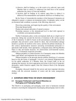
Figure 2 represents the completely mixed activated sludge model typically
found in industrial pretreatment applications. Here i, e, r, and w are used to denote
the influent, effluent, recycle, and waste conditions, respectively. Other parame-
ters include:
Q = volumetric flow rate, m
3
/d
Va = volume of the aeration tank, m
3

Copyright 2002 by Marcel Dekker, Inc. All Rights Reserved.
c = contaminant concentration, g/m
3
x = biomass concentration, g/m
3
The substrate (contaminant) and biomass material balances are used to obtain the
required operating design equations. In order to develop the substrate and biomass
material balances, the following several assumptions must be made:
Complete mixing occurs.
Influent flows and substrate concentrations are constant, i.e., the system is
at steady state.
Influent biomass (x
i
) is zero.
All of the substrate, food, is soluble.
Biological activity occurs only in the aeration tank (no substrate is removed
in the clarifier).
Sludge wasting occurs only in the clarifier.
Solids mass in clarifier and recycle line << mass solids in aeration tank (xVa ) .
3.1.1 Biomass Material Balance
Using the assumptions stated above, a material balance initially neglecting the
recycle stream is made:
Influent biomass + biomass production =
effluent biomass + wasted biomass
Q
i
x
i
+ V
dx

dt
=(Q
i
− Q
w
)x
e
+ Q
w
x
w
(1)
In order to simplify Eq. (1), relationships pertaining to the sludge age, θ
c
, and
biomass generation must be known. Depending on the wastewater, the amount of
biomass in the aeration tank is 800–6000 mg/liter. The cell age is a measure of
the average amount of time the biological solids remain in the aeration tank and
is used to help maintain the desired active biomass concentration. The sludge age
and biomass generation terms are typically expressed as shown in Eqs. (2) and
(3), respectively:
FIGURE 2 Process diagram for completely mixed activated sludge model.
Copyright 2002 by Marcel Dekker, Inc. All Rights Reserved.
θ
c
=
Vx
(dx/dt)
R
=

xV
a
Q
w
x
r
+(Q
i
− Q
w
)x
e
(2)



dx
dt



gen
= Y



dc
dt




u
− k
d
x (3)
where the k
d
x term is used to describe the amount of energy to keep the biomass
alive and Y is the true cell yield. Substituting Eqs. (2), (3), and the Monod
relationship for (dc/dt) into Eq. (1) will yield the common design equation. After
rearranging, Eq. (1) becomes
c
e
=
K(θ
c
−1
+ k
d
)
Yk − [θ
c
−1
+ k
d
]
(4)
where
K = Monod saturation constant, g/m
3

k
d
= microbial decay coefficient, d
–1
k = maximum specific substrate utilization rate, d
–1
Y = true cell growth yield, g cell produced per g cell removed
c
e
= effluent concentration, g/m
3
θ
c
= mean cell residence time, d
Using Eq. (4), the only variable is the cell age, which can be used to control the
effluent concentration. In other words, if the desired effluent is not achieved,
the cell age is increased which increases the substrate residence time, thereby
enabling the biomass to have a longer time to facilitate the substrate degradation.
3.1.2 Substrate Material Balance
One of the uses of the substrate material balance is to determine the volume of
the recycle stream required for achieving the desired effluent concentration. In
this situation, the system boundary is around the aeration tank and includes the
recycle stream.
Using the basic material balance, accumulation = in – out + generation, and
the assumptions stated previously, the substrate material balance is
Q
i
c
i
+ Q

r
c
e
=(Q
i
+ Q
r
)c
e
+



dc
dt



u
V
a
(5)
Grouping like terms and incorporating the relationship for cell age yields
θ
c
−1
+ k
d
Y
=

Q(c
i
− c
e
)
xV
a
(6)
Rearranging Eq. (6) to group process variables yields
Copyright 2002 by Marcel Dekker, Inc. All Rights Reserved.
xV
a
Q
=
Y(c
i
− c
e
)
θ
c
−1
+ k
d
(7)
Equation (7) can be further simplified by introducing the hydraulic residence
time, θ
H
:
xθ

H
=
Y(c
i
− c
e
)
θ
c
−1
+ k
d
(8)
The form given in Eq. (8) is the operating substrate design equation used by most
wastewater treatment facilities. This form allows, for a fixed effluent substrate
concentration and cell age, the hydraulic residence time and required biomass
concentration to be determined.
3.1.3 Typical Design Values and Waste Applications
As stated previously, the average initial biomass concentration for activated
sludge systems is in the range of 800–6000 mg/liter. The specific value used
depends on the food substrate (F) to microbe (M) ratio. Most F/M ratios are in
the range 0.04–0.07 [107]. The higher ratio is implemented for elevated organic
loading rates that require more microbial activity to achieve the desired effluent
concentrations. For completely mixed activated sludge systems with a 5-day cell
age, the optimal loading rate of 1 kg substrate/day/m
3
would require at least 25%
of the water to be recycled through the aeration tank.
Activated sludge systems have had demonstrated success with conventional
municipal wastewater. They have also been used for dairy waste, nonpesticide

agricultural waste, pharmaceutical waste, and low-strength singular solvents in
industrial pretreatment. Activated sludge is not effective for exotic organic
chemicals such as pesticides, high-strength solvents, elevated heavy metal con-
centrations, alkaline waters, or mixed wastes. Copper, nickel, and zinc at concen-
trations as low as 1 mg/liter have been shown to inhibit microbial activity (110).
As effluent constraints become more stringent, the applicability of basic activated
sludge systems for treating most industrial pretreatment waste streams will
decrease unless the waste streams are segregated and the biomass acclimated to
the specific waste present (111,112).
3.2 Attached Growth
Attached growth systems encompasses processes from biofilms to slime layers.
Biofilms are used for facilitating biooxidation reactions of contaminated gas
emissions. Slime layers are utilized for biofiltration.
3.2.1 Biofiltration
The two most common processes employed for biofiltration are trickling filters
(TFs) and rotating biological contactors (RBCs). For wastewater applications, the
Copyright 2002 by Marcel Dekker, Inc. All Rights Reserved.
slime layers are comprised of a mixed population of bacteria, protozoa, and fungi.
Depending on the waste constituents, the dominant species in the population will
change. Also, the protozoa are employed as an auxiliary control on the slime
thickness. If the slime layer is too large, the treatment efficiency will be decreased
due to mass transfer limitations.
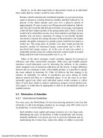
Trickling Filters. Trickling filters are not filters as their name implies, but
a means of providing a large surface area where the microbes can attach as they
“feed” on the organics. The media support is usually in the form of rocks, stones,
or ceramics, depending on the surface area and throughput required. As depicted
in Figure 3, water trickles over the top of the media to provide the contact between
the microbial population and contaminant. TFs are classified as an aerobic
treatment since aerobic cultures are responsible for over 75% of the degradation.
However, aerobic cultures are located only to a film depth of 0.1–0.2 mm; toward

the center of the media, faculative anaerobes dominate the microbial population,
as dissolved oxygen concentrations at this point are minimal (84,113,114).
TFs have had demonstrated success at both the pilot scale (for exotic
chemicals) and full scale for municipal-industrial pretreatment. At the pilot scale,
TFs in different orientations have been effective for both inorganics and organic
constituents. One study demonstrated a 94% reduction of manganese, while
another study degraded 97% of a 300-ppm styrene waste stream (115). TFs have
been used for over 30 years as a secondary or tertiary treatment for municipal
wastewater (116). Full-scale effectiveness has also be proven for some recalci-
trant organics as well. For instance, one plant was used to treat a waste stream
containing 460 mg/liter of alkyl ethoxylate sulfates and alkylbenzene sulfonates
to between 46 and 130 mg/liter (115).
FIGURE 3 General representation of a trickling filter.
Copyright 2002 by Marcel Dekker, Inc. All Rights Reserved.
The three primary design variables for TFs are the hydraulic loading rate
(HLR), organic loading rate (OLR), and recycle ratio (α). The parameters are
determined from material balances around the system shown in Figure 4 as
HLR =
Q
i
+ Q
r
A
(9)
OLR =
Q
i
c
i
+ Q

r
c
e
V
(10)
α=
Q
r
Q
(11)
Both the HLR and OLR will directly affect and the depth of media required
for treating the contaminant. As shown in Eqs. (9) and (10), OLR and HLR are
interconnected, thus providing engineers some room to manipulate actual values
and still achieve the desired effluent constraints. For instance, changing the
medium depth will increase the residence time, thereby enabling the microbes to
have greater contact with the contaminant. Varying will assist with maintaining
the biofilm thickness and minimum flow rate, dampen the OLR variation, and
increase the contact with the organics. Recirculation ratios will typically vary
from 0.4 to 4, depending on the effluent constraints. Values greater than 4 are
used to treat higher-strength waste streams. With this approach, a system with
high-strength wastewater may have a low HLR and an elevated OLR. However,
if the OLR is sustained beyond the design capacity, the filter will become clogged
and ultimately fail (106).
The first design equations for TFs were empirical. Over the past 20 years,
these equations were modified to incorporate biochemical kinetics. The most
frequently used design equation was developed by Eckenfelder (116,117) as
c
e
c
i

∗
= exp



−k



A
s
(1 +α)Q



n
za
v
m



(12)
Q c
i
Q c
e
growth area
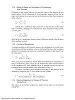
FIGURE 4 General representation of a rotating biological contactor.
Copyright 2002 by Marcel Dekker, Inc. All Rights Reserved.

where
c
e
= effluent concentration, g/m
3
c
i
* = influent concentration, including recycle, g/m
3
k = reaction rate constant, d
–1
A
s
= cross-sectional filter area, m
2
α = recycle ratio
z = filter depth, m
a
v
= specific surface area per packing piece
m, n = emperical constants determined by lab testing
Biotowers. Biotowers are the common biological treatment implemented
for minimizing waste in the dairy, milk, and food processing industries (107).
They are similar to TFs in design, operation, and use. HLR, OLR, and are still
the key design and operating parameters. The primary difference is that biotowers
use plastic media instead of the stones or rocks used in TFs. By changing the
media material to plastic, higher hydraulic and organic loading rates are obtain-
able, thus enabling biotowers to treat high-strength industrial wastes. Some
pilot-scale trials have also investigated the use of soil, granular activated carbon,
and perlite as the support material. However, polyethylene is still the primary

support/packing for biotower applications.
Biotowers have been used to treat waste streams containing more than 200
ppm of the more recalcitrant compounds. For instance, methyl ethyl ketone,
styrene, trichloromethane, and kerosene were each degraded by over 90% (82).
These efficiencies were achieved when each compound was present as the sole
contaminant. If the contaminants were present as a composite waste stream, the
biomass would have to be altered. Even with a different microbial consortium,
the remediation efficiency may not be as high, due to the degradation by products
that would be formed. Researchers are currently addressing this situation.
Based on preliminary successes, researchers are investigating the applicability of
biotowers for treating composite streams in the pharmaceutical, textile, surface
coating, and polymer processing industries (82).
Rotating Biological Contactors. Rotating biological contactors (RBCs)
employ aerobic fixed film treatment to degrade either organic or ammonia-based
constituents in wastewater. As shown in Figure 4, a RBC is comprised of a series
of corrugated disks 3–4 mm in diameter mounted on a horizontal shaft. Spacing
between the disks is in the range of 30–40 mm. Microbial slime layers forms on
the disks’ surface as they slowly rotate through the water (~1–2 rpm). The biofilm
formed on each disk is approximately 0.3–4 mm thick. A minimum of 40% of the
Copyright 2002 by Marcel Dekker, Inc. All Rights Reserved.
disk surface area is submerged in the waste stream as the RBC is rotated, to
provide the required moisture as well as to bring the microbes in contact with the
contaminants. The remaining surface area is exposed to the atmosphere, to supply
the required oxygen as well as to facilitate the biooxidation. One RBC unit can
provide up to 10,000 m
2
of surface area for biological growth.
Often, several RBCs are connected in parallel to treat the wastewater in a
timely manner. Placement of modular units in series enables the attainment of
treatment levels exceeding that of conventional secondary treatment (118).

As with TFs, Eckenfelder et al. (119) developed a relationship to determine
the removal efficiency based on contaminant concentration:
c
e
c
i
= 14.2



(Q/A)
0.558
exp(0.32N
s
)c
i
0.684
T
0.248



(13)
where
Q = mass rate of pollutant, g/d
A = disk area, ft
2
N
s
= number of RBC units used

T = water temperature, ˚C
It is important to note that Eq. (13) provides a conservative estimate for the
biodegradation efficiency, since it does not incorporate the reaction kinetics.
Eckenfelder and his associates did modify the equation to include a reaction rate
term. However, pilot-plant studies would be required to obtain the actual k value
for the specific biomass–waste combination used. Currently, the kinetic data for
RBCs are extremely limited, even for municipal wastewater applications (120).
RBCs are advantageous because they have a higher biomass concentration
than most treatment systems and are easier to operate under varying load
conditions. Unfortunately, they are prone to operational problems attributed to
biomass buildup (114). Although proven effective for low-strength organic (<1%
organic contaminants) and ammonia streams, RBCs are inefficient for high heavy
metal concentrations and complex organics such as pesticides and chlorinated
solvents (106,121). RBCs also tend to be very sensitive to temperature fluctua-
tions. For these reasons, RBCs are currently used only as secondary or tertiary
treatments.
3.2.2 Bioxidation—Scrubbing
With the newest amendment to the Clean Air Act, contaminants present in the
gas/air phase are beginning to come under closer scrutiny due to the adverse
affects they pose to human health and the environment. Part of the stricter
regulation is attributed to the acute toxicity that the contaminants pose, as well as
Copyright 2002 by Marcel Dekker, Inc. All Rights Reserved.
the fact that they are an unseen threat and disperse quickly (122). For instance,
the 1984 accidental spill in Bhopal resulted in a death toll of 2500 people in less
than 2 h. Although incidents such as that at Bhopal are not frequent, air emissions
normally released from processing facilities still pose a serious threat. These
gaseous contaminants can be efficiently and cost-effectively treated biologically
via biofilters, TFs, and bioscrubbers.
Biofilters and TFs for gaseous systems operate on the same principles as
their liquid counterparts, the only difference being the medium to be treated.

Biofilters are essentially packed beds through which the contaminated gas stream
is ventilated (14,50,123). The beds have depths of 3–4 ft and can be packed with
ceramic material, soils, plastic, or inovative materials such as volcanic rocks
(124,125). The gas enters the bottom of the bed with an upward gas velocity
ranging from 0.0005 to 0.5 ft/s and residence times of 15–60 s, depending on the
bed volume (126,127). TFs are also attached growth systems. Instead of water
being trickled through the support system, liquid nutrients and contaminated gas
are passed through (128).
Bioscrubbers are comprised of biological oxidation and an adsorption step
in which the pollutants are adsorbed to water and a bioreactor for treating the
water (129). The incorporation of thermophilic bacteria or coolants for the air
stream enables bioscrubbers to be modified and extends their applicability. With
such modifications, the adsorption column serves as both the contaminant sorp-
tion mechanisms as well as the biological support media, thereby combining the
two steps in conventional bioscrubbers (130).
As with the liquid-based approach, gas treatments employ a consortia of
bacteria instead of a pure culture. Consortiums are used since they are more
effective and often occur naturally as the introduction of new, unidentified
cultures that result from nonsterile operations (131). The combination of
seeded and unidentified cultures has resulted in 75–90% remediation of the
waste constituents, depending on the initial contaminant type and concentration
(132,133).
For instance, a biotrickling reactor developed in Germany has demonstrated
full-scale success at treating solvent-laden air. Over a 3-mo period, reactors
removed 200 g/m
3
of solvent per hour at an OLR of 600 m
3
/m
3

filter/h (134).
Other researchers have proven the ability of mixed consortia to remove over 90%
of a BTEX-contaminated off-gas (131,135). A different continuous biofilter
achieved a maximum elimination capacity of 195 g/m
3
/h for ethanol vapors (132).
Biological treatment of off-gases has also been effective for methyl tert-butyl
ether, toluene, and styrene (52,115,136). In most bioscrubbing applications, the
removal performance based on contaminant classification follows a sequence
similar to most biodegradation trends. In other words, removal rates follow the
order alcohols > esters > ketones > aromatics > alkanes (137).
Copyright 2002 by Marcel Dekker, Inc. All Rights Reserved.
4 INNOVATIVE BIOLOGICAL APPROACHES TO WASTE
MINIMIZATION
4.1 Microorganisms for Material Substitution or
By-product Utilization
Two of the key approaches to waste minimization are material substitution and
by-product utilization (138,139). If the raw material that produces the waste can
be substituted with one that either minimizes the waste or yields a viable product,
then the waste minimization goal has been realized. Furthermore, waste minimi-
zation is achievable if the intermediates or by-products of the process can also be
reused. Microorganisms have the capability to be effective vehicles for both of
these approaches, as outlined by the brief examples provided below.
4.1.1 Material Substitution
One example of a biological approach to material substitution in waste minimi-
zation is used in the formation of phenylacetylcarbinol (PAC). PAC is the key
precursor in the pharmaceutical industry for nasal decongestants. During PAC
formation, too much of a benzaldehyde intermediate is also made and disposed
of as a waste stream (140,141). Recent studies have shown that by changing the
yeast used to produce the enzyme for PAC formation, the benzaldehyde concen-

tration is lowered (142,143). Some of these studies simultaneously increased the
product yield by 140 mmol/liter (144).
p-Hydroxybenzoate (HBA) is another key raw material used in the pharma-
ceutical industry. Typically, HBA is produced by the Kolbe-Schmidt carboxyla-
tion of phenol, but this approach produces hazardous wastes (145,146).
Bioconversion of toluene via Pseudomonas putida can also produce p-HBA. In
fact, substitution with a biological approach increased the product formation
while simultaneously eliminating the hazardous intermediate(s) (147).
The two aforementioned material substitution examples are slightly differ-
ent from the nonbiological methods in that a raw material was not substituted.
Instead, the seed culture or culture for processing an intermediate was substituted
for another process. In both scenarios the bacterial substitution altered the
metabolic pathway to remove an unwanted by-product.
4.1.2 Biodegradable Polymers
Perhaps the biggest area of material substitution involves the development of
biodegradable polymers (148–150). Engineers and environmentalists know that
synthetic polymers are essentially nonbiodegradable within an acceptable
timeframe. Natural polymers, such as cellulose, proteins, starch, and poly-
dhroxyalkanoates (PHAs), can be successfully constructed from both bacteria and
plant matter (151–153). These new, natural polymers are particularly advanta-
geous to waste minimization processes since not only do they eliminate the toxic
Copyright 2002 by Marcel Dekker, Inc. All Rights Reserved.