Process Engineering for Pollution Control and Waste Minimization_11 pptx

linkage between the inventory results and effects in the environment. Others
(e.g., habitat modification) are known to play a critical role in environmental
impacts of products (e.g., agricultural products), but are difficult to model
quantitatively. Life cycle impact assessment practice is moving more and more
toward using sophisticated fate and transport models to evaluate indicators of
environmental impacts.
The choice of impact categories and category indicators and models can
drive the collection of inventory data. For example, one might choose to evaluate
only minerals whose reserves are predicted to be depleted within 100 years, or
some other reasonable time frame. This would eliminate the need to gather data
on such materials as bauxite, clay, or iron ore, and would decrease the cost of
inventory collection and management.
To date, no “standardized” listing of impact categories to be used in LCA
has been established, but several categories are employed in common practice, as
shown in Table 5.
The Classification Step. Inventory data need to be classified into the
relevant impact categories for modeling. Some emissions have influence on more
than one environmental mechanism and must be classified into more than one
category. The classic example oif this is oxides of nitrogen, or NO
x
, which acts
as catalyst in the formation of ground-level ozone (smog), but also is a source of
acid precipitation. These substances must be characterized into both categories.
One form of NO
x
(nitrous oxide, N
2
O) is also active as a greenhouse gas. The
classification rules for any LCIA must be clearly reported, so that readers of a
study understand what exactly was done to the inventory data.
The Characterization Step The goal of life cycle impact assessment is

to convert collected inventory inputs and outputs into indicators for each cate-
gory (aggregates can be system-wide, by life cycle stage, or by unit operation).
TABLE 5 Typical Impact Categories
1. Stratospheric ozone depletion
2. Global warming
3. Human health
4. Ecological health
5. Smog formation
6. Nonrenewable resource depletion
7. Land use/habitat alteration
8. Acidification
9. Eutrophication
10. Energy: processing/transportation
Copyright 2002 by Marcel Dekker, Inc. All Rights Reserved.
These indicators do not represent actual impacts, because the indicator does not
measure actual damage, such as loss of biodiversity. However, together, they do
constitute an ecoprofile for a product or service.
While there is no universally accepted “right” list of impact categories or
indicators, basic objectives have been set by the Society of Toxicology and
Chemistry (SETAC) that help define categories:
1. Category definition begins with a specific relevant endpoint. Ideally,
the endpoint can actually be observed or measured in the natural
environment.
2. Inventory data are correctly identified for collection. In principle, those
inventory inputs and outputs which relate to the particular impact are
identified.
3. An indicator describes the aggregated loading or resource use for each
individual category. The indicator is then a representation of the
aggregation of the inventory data.
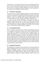
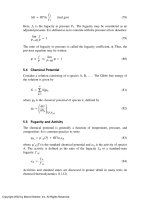
Figure 7 compares the real-world causes and effects (the environmen-

tal mechanism) with the modeled world of LCIA. There are many differences
between the two. In an LCI, for example, the inventory information is typi-
cally modeled as a constant and continuous flow, while in the real world,
emissions typically occur in a discontinuous fashion, varying from minute
to minute.
FIGURE 7 Comparison of “real-world” endpoints to LCIA indicators.
Copyright 2002 by Marcel Dekker, Inc. All Rights Reserved.
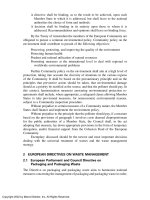
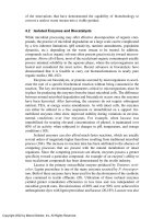
Both natural and anthropogenic flows act physically, chemically, and
biologically to produce real impacts on the biota (see Figure 8). This series of
events is called the environmental mechanism.
In the virtual reality of the environmental model, many assumptions and
simplifications are made to yield indicators. Even the best current air dispersion
models are accurate only within a factor of two to three, but the level of accuracy
is getting better all the time. The principle methodological issue in life cycle
impact assessment is the modeling management of often very complex, extended
environmental mechanisms. A listing of all possible endpoint impacts is quite
long and can look like the following suggested list.
I. Toxicity issues
A. Human health considerations
1. Acute human occupational
2. Chronic human by consumer
3. Chronic human by local population
4. Chronic human by occupational
5. Human health
6. Human toxicity by ingestion
7. Human toxicity by inhalation/dermal exposure
8. Inhalation toxicity
B. Ecological considerations
1. Aquatic toxicity
2. Biodiversity decrease

3. Endangered species extinction
4. Environmental toxicity
5. Landfill leachate (aquatic) toxicity
6. Species change
7. Terrestrial toxicity
8. Eutrophication (aquatic and terrestrial)
II. Global issues
A. Atmospheric considerations
1. Acid deposition
2. Acidification potential
3. Global warming potential
4. Stratospheric ozone depletion potential
5. Photochemical oxidation potential
6. Tropospheric ozone
B. Resource considerations
1. Energy use
2. Net water consumption
3. Nonrenewable resource depletion
Copyright 2002 by Marcel Dekker, Inc. All Rights Reserved.
FIGURE 8 Midpoints versus endpoints (20).
Copyright 2002 by Marcel Dekker, Inc. All Rights Reserved.
4. Preconsumer waste recycle percent
5. Product disassembly potential
6. Product reuse
7. Recycle content
8. Recycle potential for postconsumer
9. Renewable resource depletion
10. Resource depletion
11. Resource renewability
12. Source reduction potential

13. Surrogate for energy/emissions to transport materials to recycler
14. Waste-to-energy value
III. Local issues
A. Waste considerations
1. Airborne emissions
2. Hazardous waste
3. Incineration ash residue
4. Material persistence
5. Particulates
6. Toxic content
7. Toxic material mobility after disposal
8. Solid waste generation rate
9. Solid waste landfill space
10. Waterborne effluents
B. Public relation considerations
1. Esthetic (e.g., odor)
2. Habitat alteration
3. Heat
4. Industrial accidents
5. Noise
6. Radiation
C. Environment considerations
1. Local land
2. Local water quality
3. Physical change to soil
4. Physical change to water
5. Regional climate change
6. Regional land
7. Regional water quality
Clarifying the environmental mechanism can help determine when impacts

may be additive or when they are independent and non-additive. Two illustrative
examples are global climate change and stratospheric ozone depletion.
Copyright 2002 by Marcel Dekker, Inc. All Rights Reserved.
Example 1: Global climate change. The conversion of various greenhouse
gases into radiative equivalents is universally applicable based on a
scientifically supported mechanism (once a judgment has been made to
select a time frame for analysis.)
Example 2: Stratospheric ozone depletion. Stratospheric ozone depletion is
caused by the interaction of halogenated free radicals in the upper
atmosphere directly reducing concentrations of ozone. However, many
ozone-depleting agents are effective greenhouse gases as well. In addi-
tion, recent research indicates that greenhouse effects on the lower
atmosphere have led to trapping of energy near the earth, and consequent
cooling of the upper atmosphere. The stratospheric cooling tends to
exacerbate the effects of ozone depleters.
Nevertheless, for the purposes of LCIA models, these two mecha-
nisms are treated separately. This simplification helps develop an overall
view of the environmental impacts of industrial systems at a first-order
level. In fact, although LCIA modeling tends to be technically complex,
one can view LCIAs as extended back-of-the-envelope calculations of
realistic worst-case potential impacts.
The goal in assigning LCI results to the impact indicator categories is to
highlight environmental issues associated with each. Assignment of LCI results
should:
First assign results which are exclusive to an impact category and
Then identify LCI results that relate to more than one impact category,
including
Distinguishing between parallel mechanisms (where a given molecule
is “used up” in its actions), and serial mechanisms, where a molecule
can act in one mechanism, and then in a second mechanism without

losing its potency. SO
x
acts in parallel mechanisms of allocated be-
tween human health and acidification, while NO
x
acts in a serial mech-
anism as a catalyst in photochemical smog formation and then in
acidification.
Typically, in impact assessment a “nonthreshold” assumption is used. That
is, inventory releases are modeled for their potential impact regardless of the total
load to the receiving environment from all sources or consideration of the
assimilation capacity of the environment. However, there is a trend, particularly
in Europe, to consider thresholds in evaluating indicators. For example, ground-
level ozone formation is often calculated as an indicator for photochemical smog.
Background levels of ozone are about 20 ppb, while some vegetative damage has
been observed at 40 ppb, and human health effects at 80 ppb. All these levels, as
Copyright 2002 by Marcel Dekker, Inc. All Rights Reserved.
well as intermediate levels, have been used in determining indicators for photo-
chemical smog.
If LCI results are unavailable or of insufficient quality to achieve the goal
of the study, then either iterative data collection or adjustment of the goal is
required.
The following sections offer descriptions of current approaches that are
being applied to model some of the impact category indicators listed in Table 4.
The most simplistic models are described in order to offer insight into the types
of approaches that are being considered useful from both a practical aspect as
well as least cost.
Stratospheric Ozone Depletion. Ozone depletion is suspected to be the
result of the release of man-made halocarbons, e.g., chlorofluorocarbons, that
migrate to the stratosphere. For a substance to be considered as contributing to

ozone depletion, it must (a) be a gas at normal atmospheric temperatures,
(b) contain chlorine or bromine, and (c) be stable within the atmosphere for
several years (21).
The most important groups of ozone-depleting compounds (ODCs) are the
CFCs (chlorofluorocarbons), HCFCs (hydrochlorofluorocarbons), halons, and
methyl bromide. HFCs (hydroflourocarbons) are also halocarbons but contain
fluorine instead of chlorine or bromine, and are therefore not regarded as
contributors to ozone depletion.
The ozone depletion potential (ODP) is calculated by multiplying the
amount of the emission (Q) by the equivalency factor (EF)
ODP = Q ⋅ EF
Current status on reporting equivalency factors uses CFC11 as the reference
substance. The equivalency factor is defined as
EF
ODP
=
contribution to stratospheric ozone depletion from n over # years
contribution to stratospheric ozone depletion from CFC11
# years
General LCA practice uses values that represent ODC’s full contribution, but
Table 6 also shows factors for 5, 20, and 100 years for some gases. The ozone
depletion potential (ODP) is calculated by multiplying a substance’s mass emis-
sion (Q) by its equivalency factor. These individual potentials can then be
summed to give an indication of projected total ODP for substances 1 through n
in the life cycle inventory that contribute to ozone depletion:
ODP =
∑
n
1
(Q ⋅ EF

ODP
)
Global Warming. The most significant impact on global warming has
been attributed to the burning of fossil fuels, such as coal, oil, and natural gas.
Copyright 2002 by Marcel Dekker, Inc. All Rights Reserved.
Several compounds, such as carbon dioxide (CO
2
), nitrous oxide (N
2
O), methane
(CH
4
), and halocarbons, have been identified as substances that accumulate in the
atmosphere, leading to an increased global warming effect.
For a substance to be regarded as a global warmer, it must (a) be a gas at
normal atmospheric temperatures, and (b) either be able to absorb infrared
radiation and be stable in the atmosphere with a long residence time (in years) or
be of fossil origin and converted to CO
2
in the atmosphere (21).
Table 7 is a list of substances that are considered to contribute to global
warming. Equivalency factors, based on carbon dioxide as 1, are shown for each
substance over 20-, 100-, and 500-year spans. The choice of time scale can have
considerable effect on how global warming potential is calculated. The 100-year
time frame is often selected, unless reasons exist that indicate otherwise.
EF
GWP
=
contribution from n to global warming over # years
contribution from CO

2
to global warming over # years
TABLE 6 Equivalency Factors for Ozone Depletion (21)
Substance Formula
ODP
g CFC11/g substance
5
years
20
years
100
years ∞
CFC11 CFCl
3
1 1 1 1
CFC12 CF
2
Cl 0.82
CFC113 CF
2
ClCFCl
2
0.55 0.59 0.78 0.90
CFC114 CF
2
ClCF
2
Cl 0.85
CFC115 CF
2

ClCF
3
0.40
Tetrachloromethane CCl
4
1.26 1.23 1.14 1.20
HCFC22 CHF
2
Cl 0.19 0.14 0.07 0.04
HCFC123 CF
3
CHCl
2
0.014
HCFC124 CF
3
CHFCl 0.03
HCFC141b CFCl
2
CH
3
0.54 0.33 0.13 0.10
HCFC142b CF
2
ClCH
3
0.17 0.14 0.08 0.05
HCFC225ca CF
3
CF

2
CHCl
2
0.02
HCFC225cb CF
2
ClCF
2
CHFCl 0.02
1,1,1,-Trichlorethane CH
3
CCl
3
1.03 0.45 0.15 0.12
Methyl chloride CH
3
Cl 0.02
Halon 1301 CF
3
Br 10.3 10.5 11.5 12
Halon 1211 CF
2
ClBr 11.3 9.0 4.9 5.1
Methyl bromide CH
3
Br 15.3 2.3 0.69 0.64
Copyright 2002 by Marcel Dekker, Inc. All Rights Reserved.
TABLE 7 Equivalency Factors for Global Warming (21)
Substance Formula
GWP

g CO
2
/g substance
20
years
100
years
500
years
Carbon dioxide CO
2
1 1 1
Methane CH
4
62 25 8
Nitrous oxide N
2
O 290 320 180
CFC11 CFCl
3
5000 4000 1400
CFC12 CF
2
Cl
2
7900 8500 4200
CFC113 CF
2
ClCFCl
2

5000 5000 2300
CFC114 CF
2
ClCF
2
Cl 6900 9300 8300
CFC115 CF
2
ClCF
3
6200 9300 13000
Tetrachloromethane CCl
4
2000 1400 500
HCFC22 CHF
2
Cl 4300 1700 520
HCFC123 CF
3
CHCl
2
300 93 29
HCFC124 CF
3
CHFCl 1500 480 150
HCFC141b CFCl
2
CH
3
1800 630 200

HCFC142b CF
2
ClCH
3
4200 2000 630
HCFC225ca CF
3
CF
2
CHCl
2
550 170 52
HCFC225cb CF
2
ClCF
2
CHFCl 1700 530 170
1,1,1-Trichloroethane CH
3
CCl
3
360 110 35
Chloroform CH
3
Cl 15 5 1
Methylene chloride CH
2
Cl
2
28 9 3

HFC 134a CH
2
FCF
3
3300 1300 420
HFC 152a CHF
2
CH
3
460 140 44
Halon 1301 CF
3
Br 6200 5600 2200
Carbon monoxide
a
CO 2 2 2
Hydrocarbons (NMHC)
a
Various 3 3 3
Partly oxidized
hydrocarbons
a
Various 2 2 2
Partly halogenated
hydrocarbons
a
Various 1 1 1
a
Contributes indirectly due to conversion into CO
2

. Only compounds of petrochemical
origin.
Copyright 2002 by Marcel Dekker, Inc. All Rights Reserved.
The global warming potential (GWP) is calculated by multiplying a
substance’s mass emission (Q) by its equivalency factor. These individual poten-
tials can then be summed to give an indication of projected total GWP for
substances 1 through n in the life cycle inventory that contribute to global
warming:
GWP =
∑
n
1
(Q ⋅ EF
GWP
)
Nonrenewable Resource Depletion. This impact category models resources
that are nonrenewable, or depletable. The subcategories include:
Fossil fuels
Net non-fuel oil and gas
Net mineral resources
Net metal resources
Some models also include the energy that is inherent in a product that is made
from a petroleum feedstock in order to reflect the amount of stock that was
diverted and is no longer available for use as an energy source.
This category can also reflect land use as a resource. Land that has been
disturbed directly due to physical or mechanical disturbance can be accounted for
as a resource that is no longer available either for human use or for ecological
benefit (such as providing habitat for a certain species). Other subcategories under
the resource category include:
Net marine resources depleted

Net land area
Net water resources
Net wood resources
Scientific Certification Systems (SCS) proposes the following approach in their
Life-Cycle Stressor Effects Assessment (LCSEA) model for calculating net
resource depletion (22). The LCSEA model is based on (a) the relative rates of
depletion of the various resources and (b) the relative degree of sustainability of
the resources.
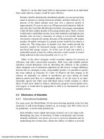
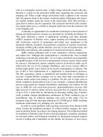
The model considers the key factors that affect resource depletion and
includes consideration of recycled material as supplementing raw material inputs.
It also takes into account materials that are part of the standing reserve base, i.e.
materials, such as steel in a bridge, that will become available as a recovered
reserve at some future time. Recycling of metals has great significance for the
depletion calculation (see Figure 9).
The elements to be considered in factoring resource depletion include:
Copyright 2002 by Marcel Dekker, Inc. All Rights Reserved.
Current world reserves
Raw material input (i.e., the amount used)
Amount recycled (both direct and standing stock)
Waste generation
Natural accretion
The reserve base-to-use ratio can be calculated as follows:
Reserve base (R)
Use (U)
= number of years of remaining use left (at current
use rate)
Use (U)
Reserve base (R)
= % of reserve base used
The recycled resource is linked to the original virgin material use and correspond-

ing reserve base. Emissions are not spatially or temporally lined to the original
virgin unit operation. Accounting for all reserve bases:
Waste (
∑
W)
Reserve base (R)+ recyclable stock (
∑
S)
The current assumption is that only one iteration of recycling and material
integrity is sustained. If natural accretion is accounted for, the following formula
results:
waste (
∑
W)− natural accretion (N)
reserve base (R)+ subsequent uses (
∑
S)
Including the time period in the equation, we get:
FIGURE 9 Flow of metals, including standing reserve.
Copyright 2002 by Marcel Dekker, Inc. All Rights Reserved.
(
∑
W − N)∆T
R +(
∑
S)∆T
Current assumption: ∆T = 50 years
And accounting for baseline reserve bases,
(
∑

W − N)∆T +(R
b
− R)
R +(
∑
S)∆T
R
b
= a reserve base baseline
Therefore,
Resource depletion factor (RDF) =
(
∑
W − N)∆T +(R
b
− R)
R +(
∑
S)∆T
Resource depletion of fossil fuels represents a simple application. Accretion is
zero and recycling is nil. Thus, wasted resource equals resource used, or
RDF =
(W)∗T
R
The impact for the resource depletion category can then be calculated according
to the formula:
Resource depletion indicator (RD) = resource use ×
resource depletion factor (RDF)
For net resources depleted (or accreted), the units of measure express the
equivalent depletion (or accretion) of the identified resource. All of the net

resource calculations are based on RDFs.
Indicator—net resource Units of measure
Water Equivalent cubic meters
Wood Equivalent cubic meters
Fossil fuels Tons of oil equivalents
Non-fuel oil and gas Tons of oil equivalents
Metals Tons of (metal) equivalents
Minerals Tons of (mineral) equivalents
Land area Equivalent hectares
Acidification. For acidification, an equivalency approach is typically ap-
plied and the stressor flows are converted into SO
2
or H
+
equivalents. For
example, NO
2
is multiplied by 64/(2 ∗ 46) = 0.70, since this is the molar proton
Copyright 2002 by Marcel Dekker, Inc. All Rights Reserved.
release potency of NO
2
compared to SO
2
. Table 8 shows sample calculations
using potency factors for an inventory with SO
2
, NO
2
, and HCl releases. The
LCSEA approach takes the calculation one step further and includes an emission

loading factor to reflect how much of the inventory release is expected to reach
the receiving environment.
Eutrophication. Eutrophication occurs in aquatic systems when the limit-
ing nutrient in the water is supplied, thus causing algal blooms. In fresh water, it
is generally phosphate which is the limiting nutrient, while in salt waters it is
generally nitrogen which is limiting. In general, addition of nitrogen alone to fresh
waters will not cause algal growth, and addition of phosphate alone to salt waters
will not cause significant effects. In brackish waters, either nutrient can cause
algal growth, depending on the local conditions at the time of the emissions.
Eutrophication is generally measured using the concentration of chloro-
phyll-a in the water. Waters with less than 2 mg of chlorophyll-a per cubic
meter (2 mg chla m
–3
) are considered “oligotrophic,” while those with 2–10 mg
chla m
–3
are considered “mesotrophic,” and those with more than 10 mg
chla m
–3
are termed “eutrophic.” Waters over 20 mg chla m
–3
are considered
“hypereutrophic.”
As waters become mesotrophic, their species assemblages change, favoring
species that grow rapidly in the presence of nutrients (“weed” species) over those
which grow more slowly. There is some indication that eutrophication in salt
waters is the source of the red tides that are a worldwide problem.
Under eutrophic conditions, the algae in the water significantly block light
passage, while in hypereutrophic conditions the amount of biomass produced is
so high that anoxic conditions occur, leading to fish kills. There are some

indications that similar sorts of effects occur in terrestrial systems as well.
The ratio of carbon to nitrogen to phosphorus in aquatic biomass is 106:16:1
(23), on an atomic basis. This ratio is the basis of combining nitrogen and
phosphorus in calculating the eutrophication potential of emissions.
(Molar quantity of nitrate + nitrite + ammonia) × Redfield ratio
+ molar quantity of phosphate × [endpoint characterization factor
(fresh, salt water)] = eutrophication indicator
Eutrophication is typically measured in PO
4
equivalents. The EPA has set a
concentration of 25 µg PO
4
L
–1
as the level needed to protect fresh-water aquatic
ecosystems from eutrophication.
Energy. While inventory analyses involves the collection of data to quan-
tify the relevant inputs and outputs of a product system, the accounting of
electricity as a flow presents a unique challenge. The use of energy audits makes
the idea of balancing energy flows around a process a familiar one. However, in
LCA the reporting of energy flows is in itself insufficient to perform a subsequent
Copyright 2002 by Marcel Dekker, Inc. All Rights Reserved.
TABLE 8
Calculating Acidification “Emission Loading” (22)
Unit operation
Inventory
emission
LCI result
(ton/30a)
Potency

factor
Molar equivalent
(ton/30a)
Characterization
factor
Emission loading
(ton/30a)
Coal mining/transport SO
2
31,620 1 31,620 0.5 15,810
NO
2
9,660 0.7 6,762 0.3 2,029
HCl 270 0.88 238 0.5 119
CaO product/transport SO
2
240 1 240 0.15 36
NO
2
1,260 0.7 882 0.075 66
Coal use SO
2
50,190 1 50,190 0.15 7,529
NO
2
36,480 0.7 25,536 0.075 1,915
HCl 15,210 0.88
13,385 0.15 2,008
Total 128,853 29,512
Copyright 2002 by Marcel Dekker, Inc. All Rights Reserved.

impact assessment. Ideally, the environmental impacts associated with energy
generation should be captured in the approach. That is, the generation of electric-
ity from fossil fuels should also show the contribution to the emission of global
warming gases, solid waste (especially coal ash), etc. This type of detail also
allows for the consideration of the use of waste materials in energy recovery
operations. Also, the calculation of energy flow should take into account the
different fuels and electricity sources used, the efficiency of conversion and
distribution of energy flows, as well as the inputs and outputs associated with
generation and use of that energy flow. In addition, a more robust assessment may
consider an evaluation of the specific sources of electrical power that are
contributed to the national energy grid on a more regional approach. This type of
consideration is important in determining local impacts. For example, electricity
that is produced in Maine is not used in California. Therefore, the impacts of
electricity generation based on a national average may not be appropriate.
In the absence of a readily available model that can convert energy-related
inventory data into potential impacts based on the fuel source, a fallback position
can be to look at the source of the total energy used and identify what percentage
is obtained from the national energy grid (which is mainly fossil fuels) and what
percentage comes from other sources, such as the burning of waste materials. At
this high-level decision point, this information is appropriate and the approach
fits the indicator-by-indicator comparison framework.
3.2.6 Weighting
Weighting, also called valuation, assigns relative weights to the different impact
indicator categories based on their perceived importance. Since there are various
TABLE 9 Equivalency Factors for Acidifiers (21)
Formula Conversion
M
w
g ⋅ mol n
EF kg SO

2
/
kg substance
SO
2
SO
2
+ H
2
O → H
2
SO
3
→ 2H
+
+ SO
3
2−
64.06 2 1
SO
3
SO
3
+ H
2
O → H
2
SO
4
→ 2H

+
+ SO
4
2−
80.06 2 0.8
NO
2
NO
2
+
1
⁄
2
H
2
O +
1
⁄
4
O
2
→ 2H
+
+ SO
3
2−
46.01 1 0.7
NO NO + O
3
+

1
⁄
2
H
2
O → H
+
+ NO
3
−
+
3
⁄
4
O
2
30.01 1 1.07
HCl HCl → H
+
+ Cl
−
36.46 1 0.88
HNO
3
HNO
3
→ H
+
+ NO
3

−
63.01 1 0.51
H
2
SO
4
H
2
SO
4
→ 2H + SO
4
2−
98.07 2 0.65
H
3
PO
4
H
3
PO
4
→ 3H
+
+ PO
4
3−
98 3 0.98
HF HF → H
+

+ F
−
20.01 1 1.6
H
2
SH
2
S +
3
⁄
2
O
2
+ H
2
O → 2H
+
+ SO
3
2−
34.03 2 1.88
NH
3
NH
3
+ 2O
2
→ H
+
+ NO

3
−
+ H
2
O 17.03 1 1.88
Copyright 2002 by Marcel Dekker, Inc. All Rights Reserved.
ways in which different individuals consider things to be important, formal
valuation methods should make this process explicit and be representative of the
individual or group making the final decision.
ISO 14042 requires that weighting of individual categories only be done
after fully disclosing unweighted indicators. When comparing two systems, the
trade-offs between impacts often require a judgment call to be made in order to
arrive at a decision.
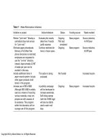
Table 10 shows the partial results of an evaluation that was conducted at
Fort Eustis, Virginia, as part of ongoing efforts to reduce waste generation from
chemical agent-resistant coating (CARC) depainting/painting operations (24).
This example focuses on a portion of the evaluation that compared the baseline
CARC system with an alternative system using a different primer and thinner
combination. The proposed switch to the alternative primer/thinner system was
identified as a possible way to reduce the facility’s air releases and potential
contribution to global climate change.
TABLE 10 Environmental Impact Scores for Baseline and
Alternative CARC Systems (24)
Spatial scale Impact category
a
Baseline Alternative
Global ODP 1.090 0.367
GLBLWRM 1.013 0.984
FSLFUELS 1.263 1.180
Regional ACIDDEP 1.198 1.175

SMOG 1.114 0.992
WTRUSE
bb
Local Toxicity:
HUMAN 2.150 1.793
ENVTERR 3.799 2.862
ENVAQ 1.280 3.540
LANDUSE 1.577 1.585
a
ODP = ozone depletion potential; GLBLWRM = global warming
potential; FSLFUELS = fossil fuel & mineral depletion potential;
ACIDDEP = acid deposition potential; SMOG = smog creation potential;
WTRUSE = water use; HUMAN = human health toxicity potential;
ENVTERR = terrestrial wildlife toxicity potential; ENVAQ = aquatic biota
potential; LANDUSE = land use for waste disposal.
b
Water use was not reported as an impact because water availability
is plentiful where CARC operations are located, and because water is
typically treated and reused or released to the environment.
Copyright 2002 by Marcel Dekker, Inc. All Rights Reserved.
After life cycle inventory data for the raw materials, painting, and disposal
of the baseline CARC and alternative system were collected, additional impact
information was then included to complete the LCA. A valuation process was
conducted on nine selected impact categories using the analytical hierarchy
process (AHP) in order to assign weights to the categories. AHP is a recognized
methodology for supporting decisions based on relative preferences of pertinent
factors.
It should be recognized that valuation is inherently a subjective process. In
the CARC study, the results of the valuation process indicated that relative to this
particular group, the greatest potential environmental concern is ozone depletion

(weight = .332). Water use was included in the valuation process, but it was not
included in the impact assessment since water is plentiful near CARC operations,
and because water is treated and reused or released to the environment. The
weights of all the impact categories (in order of decreasing importance) were
determined to be as follows:
Ozone depletion .332
Acidification .189
Global warming potential .124
Human health .099
Photochemical smog formation .097
Land use .058
Fossil fuel use .037
Water use .025
Terrestrial toxicity .020
Aquatic toxicity .020
These weights were multiplied by the normalized inventory data to arrive
at the scores shown in Table 10. For most of the impact categories, the difference
is not great enough to conclude that there is a preference between these systems.
However, for ozone depletion (ODP) and aquatic toxicity (ENVAQ), some
differences can be noted. While the ozone depletion score appears to decrease
(1.090 to 0.367), showing potential improvement, the environmental aquatic
toxicity score appears to increase (1.280 compared to 3.540). Looking back at the
inventory data, it is noted that the increased aquatic toxicity is due to increased
cadmium and chlorine releases to the wastewater associated with manufacturing
the ingredients for the alternative primer.
If the decision is made in favor of selecting the alternative system because
of its potentially lower impact on the ozone layer, it is now clear that this decision
may result in an increased burden on the wastewater system. The benefit of using
life cycle data to support the decision-making process is that the decision is being
Copyright 2002 by Marcel Dekker, Inc. All Rights Reserved.

made in a broader context and with recognition of how the production of the
alternative product can be factored in. If, on the other hand, concerns are more
immediate and focused on the local aquatic environment, with a higher weight
being assigned to aquatic toxicity, the final decision could go the other way, with
a preference for the baseline system, depending on whether the inventory data are
sufficient to influence the results in addition to an increased weight being placed
on aquatic toxicity. In either case, such weighting schemes should be made very
explicit in the final analysis.
3.2.7 Interpretation
In the interpretation step of LCA, the results of the inventory and impact modeling
are analyzed, conclusions are reached, and findings are presented in a transparent
manner. It is critical that the report that results from this activity is clear, complete,
and consistent with the goal and scope of the study. ISO 14043 lists key features
of life cycle interpretation as follows:
The use of a systematic procedure to identify, qualify, check, evaluate, and
present the conclusions based on the results of an LCA or life cycle
interpretation (LCI), in order to meet the requirements of the application
as described in the goal and scope of the study;
The use of an iterative procedure both within the interpretative phase and
with the other phases of an LCA or LCI
The provision of links between LCA and other techniques for environmen-
tal management by emphasizing the strengths and limits of an LCA study
in relation to its defined goal and scope
Transparency throughout the interpretation phase is essential. Whenever
preferences, assumptions, or value choices are used in the assessment or in
reporting, these need to be clearly stated in the final report. The goal of life cycle
interpretation is to give credibility to the results of the LCA in a way that is useful
to the decision maker.
3.3 Life Cycle Costing
Over 30 years ago, the U.S. Department of Defense recognized that operation and

maintenance (O&M) costs were substantial components of the total costs of
owning equipment and systems. In fact, ownership costs can far outweigh the costs
of procurement. By considering the full costs over the life cycle of the system and
the time value of money (e.g., discounting), better choices can be made.
The broader practice of environmental accounting now uses words such as
total cost analysis/assessment and life cycle costing to emphasize that traditional
approaches overlook important environmental costs (and potential cost savings
and revenues). A firm’s cost accounting system traditionally serves as a way to
Copyright 2002 by Marcel Dekker, Inc. All Rights Reserved.
track and allocate costs to a product or process for operational budgeting, cost
control, and pricing. In life cycle costing, accurate allocation serves to identify
environmental impacts in order to achieve pollution prevention across the entire
life cycle.
Life cycle costing has not yet achieved a single functional definition and
has been used to mean different things. However, the concept behind it refers to
the management application of environmental accounting (e.g., cost accounting,
capital budgeting, process/product design) across the life span of a product or
process. It is difficult to discern life cycle costing from total cost assessment
(TCA), because TCA is sometimes used to refer to a specific application of
environmental accounting, such as the life span of a technology or process. TCA
is often used to refer to the act of adding environmental costs into capital
budgeting, whereas life cycle costing is used more frequently when incorporating
environmental accounting into the entire design of a process or product (25).
It is essential to determine the scope of environmental costs to be included
in a life cycle costing evaluation, including not only a firm’s private costs only
(i.e., those that directly affect the firm’s bottom a line), but also private and
societal costs, some of which do not show up directly or even indirectly in the
firm’s bottom line. An expanded accounting approach is described in the EPA’s
Pollution Prevention Benefits Manual (26). The manual distinguishes among four
levels of costs:

Usual costs (Tier 0): Equipment, materials, labor, etc.
Hidden costs (Tier 1): Monitoring, paperwork, permit requirements, etc.
Liability costs (Tier 2): Future liabilities, penalties, fines, etc.
Less tangible costs (Tier 3): Corporate image, community relations, con-
sumer response, etc.
Further, there is an important distinction between costs for which a firm is
accountable and costs resulting from a firm’s activities that do not directly affect
the firm’s bottom line:
Private costs are the costs incurred by a business or costs for which a
business can be held responsible. These are the costs that directly affect
a firm’s bottom line. Private costs are sometimes termed internal costs.
Societal costs are the costs of activities, anywhere within the life cycle,
which impact on the environment and on society for which the product
manufacturer is not directly held financially responsible. These costs do
not directly affect the company’s bottom line. Societal costs are also
referred to as external costs or externalities. They may be expressed
qualitatively, in physical terms (e.g., tons of releases, exposed receptors),
or quantitatively, in dollars and cents. Societal costs can be divided as
being either environmental costs or social costs.
Copyright 2002 by Marcel Dekker, Inc. All Rights Reserved.
Life cycle costing includes all internal plus external costs incurred through-
out the life cycle of a product or process. External costs are not borne directly by
the company (or the ultimate consumer of the company’s goods or services) and
do not typically enter the company’s decision-making process. The use of
electricity can be used to demonstrate the difference between internal and external
costs. The generation of electrical power imposes various environmental impacts
and costs. Facility construction, operation, and maintenance are costs that are
incurred by the electrical generators, who recover the costs through the prices
they set to sell their electricity. Other impacts are not borne by the generator and
are not reflected in the price. For example, fossil fuel plants emit sulfur dioxide

and nitrogen oxides, precursors to acid rain. Life cycle costing would attempt to
describe qualitatively or place a dollar value on those impacts to reflect the overall
cost to society and the environment, such as human health risk, damage to
buildings and other structures (e.g., statues), damage and loss of trees and other
plant life, alteration of habitat and resulting animal species loss, etc.
Uncovering and recognizing environmental costs associated with a product,
process, system, or facility is an important goal for making good management
decisions. Attaining such goals as reducing environmental expenses, increasing
revenues, and improving future environmental performance requires paying
attention to current and potential future environmental costs. Whether or not a
cost is “environmental” is not critical; the goal is to ensure that relevant costs
receive appropriate attention.
Inherent in life cycle costing are the same considerations that were dis-
cussed in conducting a life cycle inventory: costs that are omitted may skew the
results. Also, life cycle costing cannot be used to compare disparate products, but
it is a tool for assessing comparable products or processes. Further, the function
of the products being compared should be equivalent.
4 CONCLUSIONS
Pollution prevention is a valuable concept for facility managers tasked with
environmental protection. It is a method that allows them to think about their
operations and identify opportunities to improve their operations. The main goal
of pollution prevention is to reduce or eliminate the creation of pollutants and
wastes at the source in order to reduce costs and to meet or exceed federal and
state regulations on environmental discharges and emissions. Over the years,
significant work has been done by various government offices, universities, and
industry to demonstrate pollution prevention techniques and effectively transfer
this information to wider audiences for implementation. A wealth of material on
case studies for many different industrial sectors can be found in the open
literature on this subject.
Copyright 2002 by Marcel Dekker, Inc. All Rights Reserved.

A life cycle perspective in combination with pollution prevention elevates
the concept by looking beyond a single process or facility to encompass the
environmental aspects that may be affected somewhere else within the entire
system. This type of holistic approach to identifying secondary consequences
leads the thought process toward sustainability rather than simple environmental
protection. It is LCA’s key message and the reason why LCA is becoming widely
accepted as the basis for approaches to environmental management. The system-
atic application of life cycle thinking in all aspects of decision making, including
process improvement, product selection, and end-of-life management, provides a
stronger model for environmental management than does simple pollution pre-
vention. The information that an LCA provides allows for better-informed deci-
sion making to occur. As a result, LCA is an environmental management tool and
model that is quickly being adopted at the international level. The LCA provides
information that is useful not only to the individual facility or corporation but to
environmental policy makers in governments.
LCA is a relatively recent technique in environmental protection and
sustainability, but much has been learned in the relatively short period of time
that has been dedicated to this subject. It is increasingly obvious that life
cycle-based approaches are needed to fully evaluate environmental impacts in all
our decisions and choices. The wide spectrum of activities involved in a product
or process requires that practitioners and method developers test new ways to
model LCA and exchange information among themselves and share it with
potential users (i.e., environmental decision makers) in order to advance the
understanding and application of LCA. LCA is an evolving tool that continues to
improve as better site-specific models become coupled with simpler ways to com-
municate results to the users of life cycle data.
REFERENCES
1. Harry Freeman, Pollution Prevention. In Harry M. Freeman (ed.), Industrial Pollution
Prevention Handbook. New York: McGraw-Hill, 1995.
2. L. Case, L. Mendicino, and D. Thomas, Developing and Maintaining a Pollution

Prevention Program. In Harry M. Freeman (ed.), Industrial Pollution Prevention
Handbook. New York: McGraw-Hill, 1995.
3. U.S. Environmental Protection Agency, Facility Pollution Prevention Guide, EPA/
600/R-92/088. Cincinnati, OH: Risk Reduction Engineering Laboratory, May 1992.
4. The Society of Environmental Toxicology and Chemistry, Life-Cycle Impact Assess-
ment: The State-of-the-Art, Larry Barnthouse, Jim Fava, Ken Humphreys, Robert
Hunt, Larry Laibson, Scott Noesen, James Owens, Joel Todd, Bruce Vigon, Keith
Weitz, John Young (eds.), Pensacola, FL: SETAC Foundation, 1997.
5. U.S. Environmental Protection Agency, Developing and Using Production-Adjusted
Copyright 2002 by Marcel Dekker, Inc. All Rights Reserved.
Measurements of Pollution Prevention, EPA/600/R-97/048. Cincinnati, OH: National
Risk Management Research Laboratory, September 1997.
6. David P. Evers, Facility Pollution Prevention Planning. In Harry M. Freeman (ed.),
Industrial Pollution Prevention Handbook. New York: McGraw-Hill, 1995.
7. U.S. Environmental Protection Agency, Development of Computer Supported Infor-
mation System Shell for Measuring Pollution Prevention Progress, EPA/600/R-
95/130, NRMRL, Cincinnati, OH: National Risk Management Research Laboratory,
August 1995.
8. B. W. Baetz, E. I. Pas, and P. A. Vesiland, Planning Hazardous Waste Reduction and
Treatment Strategies: An Optimization Approach. Waste Manage. Res., vol.7, no. 2,
pp. 153–163, 1989.
9. Kenneth Humphreys and Paul Wellman, Basic Cost Engineering. New York: Marcel
Dekker, 1996.
10. International Standards Organization, Environmental Management—Life Cycle
Assessment—Principles and Framework, ISO 14040, 1997.
11. International Standards Organization, Environmental Management—Life Cycle
Assessment—Goal and Scope Definition and Inventory Analysis, ISO 14041, 1998.
12. International Standards Organization, Environmental Management—Life Cycle
Assessment—Life Cycle Impact Assessment, ISO 14042, 2000.
13. International Standards Organization, Environmental Management—Life Cycle

Assessment—Life Cycle Interpretation, ISO 14043, 2000.
14. J.A. Fava, R. Denison, B. Jones, M. A. Curran, B. W. Vigon, S. Selke, and J. Barnum
(eds.), A Technical Framework for Life Cycle Assessments. Pensacola, FL: The
Society of Environmental Toxicology and Chemistry, 1991.
15. K. Stone and J. Springer, Review of Solvent Cleaning in Aerospace Operations and
Pollution Prevention Alternatives, Environ. Prog., vol. 14, no. 4, pp. 261–272, 1995.
16. U.S. Environmental Protection Agency, Streamlined Life-Cycle Assessment of 1,4-
Butanediol Produced from Petroleum Feedstocks versus Bio-Derived Feedstocks, in
Cincinnati, OH: National Risk Management Research Laboratory, September 1997.
17. The Society of Environmental Toxicology and Chemistry, Streamlined Life Cycle
Assessment, Joel Ann Todd and Mary Ann Curran (eds.), Pensacola, FL, June 1999.
18. U.S. Environmental Protection Agency, Life Cycle Assessment: Inventory Guidelines
and Principles, EPA/600/R-92/245. Cincinnati, OH: Risk Reduction Engineering
Laboratory, February 1993.
19. U.S. Environmental Protection Agency, Life-Cycle Impact Assessment: A Conceptual
Framework, Key Issues, and Summary of Existing Methods. prepared by the Research
Triangle Institute (RTI), July 1995.
20. U. de Haes, O. Jolliet, G. Finnveden, M. Hauschild, W. Krewitt, and R. Mueller-
Wenk, Best Available Practice Regarding Impact Categories and Category Indicators
in Life Cycle Impact Assessment, SETAC Life Cycle Impact Assessment Workgroup
discussion paper, February 1999.
21. Henrik Wenzel, Michael Hauschild, and Leo Alting, Environmental Assessment of
Products, London, UK: Chapman & Hall, 1997.
22. S. Rhodes, F. Kommonen, and R. Schenck, Evolution of Life-Cycle Assessment as
an Environmental Decision-Making Tool: ISO 14042 and Life Cycle Stressor Efforts
Assessment (LCSEA), Workshop booklet, February 1998.
Copyright 2002 by Marcel Dekker, Inc. All Rights Reserved.
23. A. C. Redfield, The Process of Determining the Concentration of Oxygen, Phosphate,
and Other Organic Derivatives within the Depths of the Atlantic Ocean. Pap. Phys.
Ocean. Meteor. 9, 1942.

24. U.S. Environmental Protection Agency, Life Cycle Assessment for Chemical Agent
Resistant Coating, EPA/600/R-96/104, prepared by Battelle and Lockheed-Martin for
the National Risk Management Research Laboratory, Cincinnati, OH, 1996.
25. Allen White, D. Savage, and K. Shapiro, Life Cycle Costing: Concepts and Applica-
tions. In M. A. Curran (ed.), Environmental Life Cycle Assessment. New York:
McGraw-Hill, 1996.
26. U.S. Environmental Protection Agency, Pollution Prevention Benefits Manual, EPA230/
R-98/100, October 1989.
27. U.S. Environmental Protection Agency, Pathway to Product Stewardship: Life-Cycle
Design as a Business Decision-Support Tool, EPA/742/R-97/008. Office of Pollution
Prevention and Toxics, December 1997.
GLOSSARY
Functional unit The measure of a life cycle system used to base reference
flows in order to calculate inputs and outputs of the system
Inventory See Life cycle inventory.
ISO International Standards Organization (or International Organization
of Standardization).
Life (1) Economic: that period of time after which a product, machine, or
facility should be discarded because of its excessive costs or reduced
profitability. (2) Physical: that period of time after which a product,
machine, or facility can no longer be repaired in order to perform its
designed function properly.
Life cycle assessment Evaluation of the environmental effects associated
with any given activity from the initial gathering of raw materials from
the earth to the point at which all materials are returned to the earth; this
evaluation includes all releases to the air, water, and soil.
Life cycle cost The sum of all discounted costs of acquiring, owning,
operating, and maintaining a project over the study period (i.e., the life
of the product or process). Comparing life cycle costs among mutually
exclusive projects of equal performance has been used as a way to

determine relative costs.
Life cycle impact assessment A scientifically based process or model
which characterizes projected environmental and human health impacts
based on the results of the life cycle inventory.
Life cycle inventory An objective, data-based process of quantifying
energy and raw material requirements, air emissions, waterborne efflu-
ents, solid waste, and other environmental releases throughout the life
cycle of a product, process, or activity.
Copyright 2002 by Marcel Dekker, Inc. All Rights Reserved.
Pollution prevention The use of materials, processes, or practices that
reduce or eliminate the creation of pollutants or wastes at the source.
Pollution prevention opportunity assessment The systematic process of
identifying areas, processes, and activities which generate excessive
waste streams or waste by-products for the purpose of substitution,
alteration, or elimination of the waste.
POTW (Publicy Owned Treatment Works) Any device or system used
to treat (including recycling and reclamation) municipal sewage or
industrial wastes of a liquid nature that is owned by a state, municipality,
intermunicipality, or interstate agency [defined by Section 502(4) of the
Clean Water Act].
RCRA (Resource Conservation and Recovery Act of 1976) Amending
the Solid Waste Disposal Act (SWDA), the RCRA established a regula-
tory system to track the generation of hazardous substances from the time
of generation to disposal. The U.S. Congress declares it to be the national
policy of the country that, whenever feasible, the generation of hazardous
waste is to be reduced or eliminated as expeditiously as possible. Waste
that is nevertheless generated should be treated, stored, or disposed of so
as to minimize the present and future threat to human health and the
environment (40 USC 6902).
Waste minimization Approaches or techniques that reduce the amount of

RCRA-regulated wastes generated during industrial production pro-
cesses; the term applies to recycling and other efforts to reduce waste
volume.
Copyright 2002 by Marcel Dekker, Inc. All Rights Reserved.
16
Application of Life Cycle Assessment
W. David Constant
Louisiana State University and A&M College, Baton Rouge, Louisiana
1 INTRODUCTION
Application of life cycle assessment (LCA) ensures that environmental impact is
explicitly included in the design process, yielding the “best” alternative. The
“best” choice can be difficult in the final analysis to assess, as many factors may
cause an objective LCA to fall into a gray or subjective area. Graedel (1) presents
an excellent methodology for streamlined LCA with a matrix approach, yielding
objective results, and explores the approaches used by major manufacturers in
obtaining data for the matrices. Others (2,3) present basic studies and applica-
tions, and there are many articles and texts available between basics and detailed
methods. The objective of this chapter is to explore the application of LCA for
waste site remediation, as an example of the extension of LCA to areas beyond
manufacturing goods and consumer products.
2 BASICS FROM CHEMICAL ENGINEERING
Application of LCA to assess a waste site remedy is making use of the basics of
chemical engineering and related fields, the material and energy balances, with a
few other topics included, such as economics, eco- and/or health risk assessment,
Copyright 2002 by Marcel Dekker, Inc. All Rights Reserved.