MIMO Systems Theory and Applications Part 2 ppt

0 5 10 15 20
0
5
10
15
20
25
SNR (dB)
MIMO Capacity (bits/s/Hz)


Uniform power allocation
Optimal power allocation
Optimal power allocation (Uncorrelated MIMO channel)
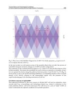
Fig. 12. MIMO(4 ×4): Capacity improvement with WF strategy-Channel correlation impact
on system capacity
2 4 6 8 10 12 14
0
0.1
0.2
0.3
0.4
0.5
0.6
0.7
0.8
0.9
1
Capacity(bits/s/Hz)
P(C> abscisse)

NoWF−SNR=6dB
NoWF−SNR=10dB
WF−SNR=6dB
WF−SNR=10dB
SNR=6dB
SNR=10dB
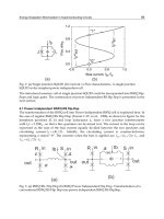
Fig. 13. CCDF for MIMO(4 ×4) with various SNR values
24
MIMO Systems, Theory and Applications
0 5 10 15 20
2
4
6
8
10
12
14
SNR (dB)
MIMO Capacity (bits/s/Hz)


No WF
WF
Fig. 14. Ergodic capacity for MIMO(4 ×2)-Kronecker channel model
4 5 6 7 8 9 10 11 12
0
0.1
0.2
0.3

0.4
0.5
0.6
0.7
0.8
0.9
1
Capacity (bits/s/Hz)
P(C> abscisse)


NoWF
WF
Fig. 15. CCDF for MIMO(4 ×2)-Kronecker channel model (SNR=18dB)
25
Advanced MIMO Techniques: Polarization Diversity and Antenna Selection
0.5 1 1.5 2 2.5 3 3.5 4 4.5 5 5.5
0
0.1
0.2
0.3
0.4
0.5
0.6
0.7
0.8
0.9
1
Capacity (bits/s/Hz)
P(C>abscisse)

NoWF
WF
Fig. 16. CCDF for MIMO(4 ×2)-Kronecker channel model (SNR=2dB)
6. Combining techniques for MIMO systems
MIMO system can use several techniques at the receiver so that to combine the multiple
incoming signals for more robust reception. Combining techniques are listed below :
1. Maximal Ratio Combining (MRC): Incoming signals are combined proportional to the SNR
of that path signal. The MRC coefficients correspond to the relative amplitudes of the pulse
replicas received by each antenna such that more emphasis is placed on stronger multipath
components and less on weaker ones.
2. Equal Gain Combining (EGC) simply adds the path signals after they have been cophased
(Sanayei & Nosratinia, 2004).
3. Selection Combining (SC) selects the highest strength of incoming signals from one of the
receiving antennas.
Combining techniques can be carried so that to satisfy one or more targets :
1. Maximizing the diversity gain
2. Maximizing the multiplexing gain
3. Achieving a compromise between diversity gain and multiplexing gain
4. Achieving best performances in terms of Bit Error Rate (BER)
5. Maximizing the Frobenius norm of the MIMO channel and therefore the MIMO channel
capacity
Let us recall the SIMO system model with N
R
receive antennas. The received signal at the q-th
receive antenna is expressed as :
y
q
= h

q
x + b
q
; q = 1, ,N
R
(60)
h
q
is the q-th complex channel gain, b
q
is an AWGN with zero mean and variance σ
2
b
.
We keep for notations :
26
MIMO Systems, Theory and Applications
• P
T
: Transmit signal power
• γ
=
P
T
σ
2
b
is the SNR
We assume channel normalization and a perfect channel estimation. We will be more
interested in the combining module. Our aim is to derive the combining coefficients g

q
; q =
1, ,N
R
. The output signal at the combining module can be expressed as:
y
= x
N
R
∑
q =1
g
q
h
q
+
N
R
∑
q =1
g
q
b
q
(61)
Combining technique in MIMO system is depicted in Fig.17. Combining coefficients relative
to the listed techniques are given by:
Combining technique Combining coefficient
MRC g
q

= h
∗
q
EGC g
q
=
h
∗
q
|h
q
|
SC g
q
=

1,


h
q



|
h
k
|
, ∀k = q;
0, otherwise.

Table 1. Combining coefficients
Rx
1
Rx
N
R
Rx
q
Tx
p
x
⊕
⊕
⊕
⊗
⊗
⊗
❄
❄
❄
❄
❄
❄
b
1
b
N
R
b
q

g
1
g
N
R
g
q
✲
✲
✲
✲
✲
✲
∑
✍✌
✎☞
✇
✲
✲
y
.
.
.
.
.
.
.
.
.
.

.
.
.
.
.
.
.
.
✼
✼
✲
⑦
✲
Fig. 17. SIMO system with combining technique
6.1 Maximal Ratio Combining (MRC)
The equivalent SNR of MRC has been calculated as :
γ
y
= γ ·

N
R
∑
q =1


h
q



2

2
N
R
∑
q =1


h
q


2
= γ ·
N
R
∑
q =1


h
q


2
=
N
R
∑

q =1
γ
q
(62)
Thus, the instantaneous SNR γ
y
is expressed as the sum of the instantaneous SNR at different
receive antennas. For normalized channel matrix, the SNR is then:
γ
y
= N
R
·γ (63)
27
Advanced MIMO Techniques: Polarization Diversity and Antenna Selection
The system capacity with MRC is :
C
MRC
= log
2

1
+ γ ·
N
R
∑
q =1


h

q


2

bit s/s/Hz (64)
6.2 Equal Gain Combining (EGC)
The instantaneous SNR is expressed as :
γ
y
=
γ
N
R
·

N
R
∑
q =1
|h
q
|

2
(65)
Resulting capacity has been calculated as :
C
EGC
= log

2

1
+
γ
N
R
·
N
R
∑
q =1


h
q


2

bit s/s/Hz (66)
6.3 Selection Combining(SC)
The receiver scans the antennas, finds the antenna with the highest instantaneous SNR and
selects it. We denote the highest received instantaneous SNR as :
γ
y
= max
(
γ
1

, ,γ
N
R
)
(67)
The SNR at the output of the combiner for an uncorrelated channel is:
γ
y
= γ ·
N
R
∑
q =1
1
q
(68)
SC capacity is expressed as:
C
SC
= log
2

1
+ γ ·max
q


h
q



2

= max
q

log
2

1
+ γ ·


h
q


2

;1
≤ q ≤ N
R
bit s/s/Hz (69)
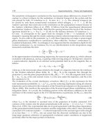
The ergodic capacity curves for all three combining strategies are shown in Fig. 18. MRC yields
best performances in terms of channel capacity. However, MRC is the optimal combining
technique, MRC is seldom implemented in a multipath fading channel since the complexity
of the receiver is directly resolvable paths (Zhou & Okamoto, 2004). In general, EGC performs
worse than does MRC. Obviously, lower capacity is obtained with SC since only one Radio
Frequency (RF) channel is selected at the receiver. A study of combining techniques in
terms of BER was presented in (Zhou & Okamoto, 2004). MRC steel achieves the best BER

performances.
7. Beamforming processing in MIMO systems
Beamforming is the process of trying to steer the digital baseband signals to one particular
direction by weighting these signals differently. This is named "digital beamforming" and
we call it beamforming for the sake of brevity, (Jafarkhani, 2005). The desired signal is then
obtained by summing the weighted baseband signals.
28
MIMO Systems, Theory and Applications
0 1 2 3 4 5 6 7 8
10
−7
10
−6
10
−5
10
−4
10
−3
10
−2
10
−1
SNR(dB)
BER


L
R
=1

L
R
=3
L
R
=4
Fig. 18. Capacity for MIMO(4 ×1) using various combining techniques-Rayleigh fading
channel
7.1 Beamforming based on SVD decomposition
In this section, we provide an overview of MIMO systems that use beamforming at both
the ends of the communication link. We consider a MIMO system with N
T
transmit
and N
R
receive dimensions. From a mathematical point of view, joint Transmit-Receive
beamforming is based on the minimization (or maximization) of some cost function such as
SNR maximization. This method includes determining the transmit beamforming coefficients
and the receive beamforming coefficients so that to steer relatively all transmit energy and
receive energy in the directions of interest. Joint Transmit-Receive beamforming is illustrated
in Fig. 19.
Rx
1
Tx
1
Rx
N
R
Tx
N

T
Rx
q
Tx
p
⊕⊗
⊕⊗
⊕⊗
⊗
⊗
⊗
❄❄
❄❄
❄❄
❄
❄
❄
b
1
Wt
1
b
N
R
Wt
N
T
b
q
Wt

p
Wr
1
Wr
N
R
Wr
q
✲
✲
✲
✲
✲
✲
∑
✍✌
✎☞
✇
✲
y
BF
.
.
.
.
.
.
.
.
.

.
.
.
.
.
.
.
.
.
.
.
.
.
.
.
.
.
.
.
.
.
✼
✲
✲
✲
✲
✲
✲
✲
x

✶
✶
✶
q
q
q
Fig. 19. Joint Transmit-Receive beamforming
• x: The transmit signal
• Wt
=[Wt
1
,. ,Wt
N
T
]
T
:The(N
T
×1) Transmit beamforming vector
29
Advanced MIMO Techniques: Polarization Diversity and Antenna Selection
• H:The(N
R
×N
T
) channel matrix
• Wr
=[Wr
1
, ,Wr

N
R
]
T
:The(N
R
×1) Receive beamforming vector
• b
=[b
1
, ,b
N
R
]
T
:The(N
R
×1) Additive noise vector with variance σ
2
b
• y
BF
: The output signal
Joint Transmit-Receive beamforming can be described by equation (70).
y
BF
= Wr
H
HW
t

·x + Wr
H
·b (70)
Eigen-beamforming could be performed by using eigenvectors to find the linear beamformer
that optimizes the system performances. Thus, we exploit the SVD factorization for channel
matrix H (H
= USV
H
). Assigning U and V respectively to Wr and Wt is optimal for
maximizing the SNR given by :
SNR
BF
=

Wr
H
HWt
2
E(xx
H
)
σ
2
b
Wr
2
When SVD factorization is applied to MIMO channel matrix, equation (70) becomes :
y
BF
= S ·x + U

H
·b (71)
Note that Beamforming (Ibnkahla, 2009) is considered as a form of linear combining
techniques which are intended to maximize the spectral efficiency. The received SNR for
communication system with beamforming is expressed as :
γ
BF
= γ
r
·λ
max
(H)
λ
max
is the maximum eigenvalue associated to matrix S and γ
r
is the mean received SNR.
Thereafter, the capacity for MIMO system with beamforming is expressed as :
C
BF
= log
2
{
1 + γ
r
·λ
max
(H)
}
bit s/s/Hz (72)

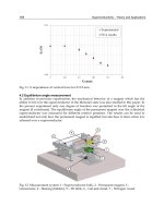
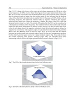
Simulation results for MIMO capacity where beamforming technique is performed are shown
in Fig. 20. The MIMO channel capacity with beamforming is improved thanks to the spatial
diversity.
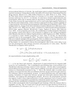
Note that beamforming technique is shown to improve the performance of the communication
link in terms of BER. Fig. 21 shows the plotted curves of BER as a function of SNR relative to
three cases :
• System performing beamforming
• Transmission without applying beamforming
• Transmission with simply Zero Forcing (ZF) equalization
The MIMO
(3 ×3) channel is randomly generated and input signal is BPSK modulated. We
adopt the correlated MIMO channel with a spreading angle of 90
◦
and an antenna spacing of
λ
2
. Fig. 21 shows that associated SVD beamforming technique brings the best performances in
terms of BER.
30
MIMO Systems, Theory and Applications
0 5 10 15 20
1
2
3
4
5
6
7
8
9

10
11
SNR(dB)
Capacity(bits/s/Hz)


SISO
MIMO(2X2)
MIMO(3X3)
MIMO(4X4)
Fig. 20. Capacity of MIMO system with beamforming technique
0 2 4 6 8 10
10
−3
10
−2
10
−1
10
0
SNR (dB)
BER


BF
NoBF
ZF
Fig. 21. SVD based beamforming technique
31
Advanced MIMO Techniques: Polarization Diversity and Antenna Selection

7.2 SINR maximization beamforming
Interference often occurs in wireless propagation environment. When several terminals are
densely deployed in the coverage area, Signal to Interference Noise Ratio (SINR) grows up
and efficient techniques are required to be implemented. Beamforming is an efficient strategy
that could be exploited so that to mitigate interference. Maximizing the SINR criteria could be
also considered so that to obtain optimal beamforming weights.
SINR maximization based beamforming in Multi user system
Model description
Rx
1
Tx
1
Rx
1
Rx
M
1
Tx
N
Rx
M
K
.
.
.
.
.
.
.
.

.
.
.
.
U
K
U
1
BS
✿
✸
③
✿
✬
✫
✩
✪
❘
✇
q
⑦
✬
✫
✩
✪
H
K
H
1
♥

+
❫
✣
♠
♠
×
×
✲
✲
❄
Wt
1
Wt
K
e
1
e
K
.
.
.
ˆe
1
ˆe
K
.
.
.
❄
✲

✲
Fig. 22. Multi user system with beamforming
We denote :
• K:Numberofusers.
• E
=[e
1
, ,e
N
]
T
: The transmit signal vector
• Wt=
[Wt
1
, ,Wt
K
]
T
: Weight vector for beamforming
• M
1
, ,M
K
number of antennas respectively for users U
1
, ,U
K
• x: The transmit vector signal of size (N ×1)
Transmit signal is expressed as :

x
=
K
∑
k= 1
Wt
k
·e
k
(73)
We assume that transmit signals and beamforming weights are normalized. The received
signal (Of size
(M
i
×1))byuserU
i
is :
y
i
= H
i
K
∑
k= 1
Wt
k
·e
k
+ b
i

(74)
32
MIMO Systems, Theory and Applications
b
i
is the additive noise with variance σ
2
i
. The channel matrix H
i
(M
i
×N) between user U
i
with
M
i
antennas and the N antennas at the Base Station (BS) is assumed to be normalized. User
U
i
; i = 1, ,K receives the signal :
y
i
= H
i
Wt
i
·e
i
+

K
∑
k= 1,k =i
H
i
Wt
k
·e
k
+ b
i
(75)
At the receiver, the estimated signal for user i is:
ˆe
i
=
Wt
H
i
H
H
i
y
i
H
i
Wt
i

(76)

The SINR is the ratio of the received strength of the desired signal to the received strength of
undesired signals (Noise + Interference). Associated SINR to user i is expressed as :
SINR
i
=

H
i
Wt
i

2

K
∑
k=1,k=i
 H
i
Wt
k

2

+ σ
2
i
(77)
SINR could also be written as :
SINR
i

=

H
i
Wt
i

2
⎛
⎜
⎝
K
∑
k=1,k=i
Wt
H
i
H
H
i
H
i
Wt
k

2
H
i
Wt
i


2
⎞
⎟
⎠
+ σ
2
i
(78)
Optimal beamformer weights are obtained by maximizing the Signal Leakage Ratio (SLR)
metric expressed as :
SLR
=

H
i
Wt
i

2

˜
H
i
Wt
i

2
(79)
where :

˜
H
i
=[H
H
1
, ,H
H
i
−1
,H
H
i
+1
, ,H
H
K
]
H
(80)
The optimal weights Wt
i
; i = 1, ,K are derived (Tarighat et al., 2005) as the maximum
eigenvector of:
((
˜
H
i
H
˜

H
i
)
−1
(H
H
i
H
i
))
Simulation results are shown in Fig. 23. These results show that the method is optimal for
determining the beamforming weights. Note that better performances in terms of BER are
achieved if more transmit antennas are used.
33
Advanced MIMO Techniques: Polarization Diversity and Antenna Selection
0 1 2 3 4 5 6 7 8
10
−4
10
−3
10
−2
10
−1
SNR(dB)
BER


M=4
M=3

Fig. 23. Multi user BF (K = 3, M = 3/M = 4)
8. Processing techniques for MIMO systems: Antenna selection
MIMO system gives high performances in terms of system capacity and reliability of
radio communication. Combining techniques such as MRC results in more robust system.
Nevertheless, the deployment of multiple antennas would require the implementation of
multiple RF chains (Dong et al., 2008). This would be costly in terms of size, power and
hardware. For example, when several antennas are deployed, multiple RF chains with
separate modulator and demodulator have to be implemented. To overcome these limitations,
antenna selection techniques can be applied.
8.1 Antenna selection
Antenna selection technique (Ben ZID et al., 2011) is depicted in Fig. 24. We consider a MIMO
system with N
T
transmit antennas and N
R
receive antennas. The idea of antenna selection is
to select L
T
antennas among the N
T
transmit antennas and / or L
R
antennas among the N
R
receive antennas. We distinguish different forms of antenna selection:
1. Transmit antenna selection
2. Receive antenna selection
3. Hybrid antenna selection: that is when antenna selection is carried among both transmit
antennas and receive antennas.
Tx Rx

Tx
1
Rx
1
Tx
N
T
Rx
N
R
✲
✲
.
.
.
.
.
.
.
.
.
.
.
.
.
.
.
.
.
.

✣
✣
❥
❥
RF
RF
RF
RF
Chain
Chain
Chain
Chain
1
L
T
L
R
1
☎
✆
✕
✞
✝
❑
Fig. 24. Antenna selection in MIMO system
34
MIMO Systems, Theory and Applications
Antenna selection algorithms do not only aim to reduce the system complexity but also to
achieve high spectral efficiency. When L
T

antennas are selected at the transmitter and L
R
antennas are selected at the receiver, the associated channel will be denoted H
S
. The capacity
of such system is expressed as :
C
Sel
= log
2

det

I
L
T
+
γ
L
R
H
H
S
H
S

= log
2

det


I
L
R
+
γ
L
T
H
S
H
H
S

(81)
γ denotes the SNR. The antenna selection algorithm is intended to find the optimal subset
of the transmit antennas and /or the optimal subset of the receive antennas that satisfy
capacity system maximization. Nevertheless, it is obvious that the joint antenna selection
at the transmitter and the receiver brings more complexity when the number of antennas
increases.
Numerical results
Ergodic capacity of MIMO system with antenna selection at the transmitter and the receiver
is shown in Fig. 25. For simulation purposes, we generate a Rayleigh MIMO channel with
AWGN. Here, SVD factorization is applied. Plotted curves depict the ergodic capacity for the
MIMO
(4 ×4). This evidently leads to the highest system capacity. When 3 transmit antennas
are selected among 4 transmit antennas and 3 receive antennas are selected among 4 receive
antennas, the maximum ergodic capacity that could be achieved is plotted in function of SNR.
Simulation results are also presented in the case when two antennas are selected at both the
transmitter and the receiver. According to the plotted curves in Fig. 25, it is obvious that one of

the important limitations of the antenna selection strategy is the important losses in capacity
at high SNR regime.
0 5 10 15 20
5
10
15
20
25
30
35
SNR(dB)
Ergodic capacity


AS (2 Among 4)
AS (3 Among 4)
No AS
Fig. 25. Antenna selection in MIMO (4 ×2): Impact on ergodic capacity
35
Advanced MIMO Techniques: Polarization Diversity and Antenna Selection
8.2 Antenna selection inv olving ST coding
We present in this paragraph, the simulation results in terms of average BER when joint
Alamouti scheme and antenna selection at the receiver are applied. The MIMO
(4 ×2) system
with a Rayleigh channel and AWGN was created. Emitted symbols are QAM (Quadrature
Amplitude Modulation) modulated. The simulation model is given by the Fig. 26 (b
1
, ,b
N
R

denote the additive noise signals). Plotted curves concern subsets of receive antennas where
L
R
= 1andL
R
= 3. Simulation results show that even with only one selected antenna at the
Rx
1
Rx
N
R
Rx
q
Tx
1
Tx
N
T
⊕
⊕
⊕
❄
❄
❄
b
1
b
N
R
b

q
✲
✲
✲
✲
✲
✲
.
.
.
.
.
.
.
.
.
.
.
.
✣
⑦
✲
✲
1
L
R
.
.
.
ST

decoder
Alamouti
encoder
Antenna
selection
Input
Output
✲ ✲
Sequence
Sequence
Fig. 26. MIMO system with antenna selection and Alamouti coding
0 1 2 3 4 5 6 7 8
10
−7
10
−6
10
−5
10
−4
10
−3
10
−2
10
−1
SNR(dB)
BER

L
R
=1
L
R
=3
L
R
=4
Fig. 27. Joint Alamouti coding and antenna selection in MIMO (4 ×2)
receiver, performances in terms of BER still satisfactory. Nevertheless, when more antennas
are selected, better BER values are achieved thanks to receive diversity.
36
MIMO Systems, Theory and Applications
Tx
Rx
②
①
②
②
③
❥
③
✿
Δ
R
Scatterers
❘
✯
✒

Fig. 28. Angle spread
8.3 Antenna selection in correlated MIMO channel: Angular dispersion and channel
correlation
Angle spread refers to the spread of DOA of the multipath components at the transmit antenna
array. When scatterers are also distributed around the receive antennas, the scattering effect
leads also to an angle spreading relative to the DOA. In Fig. 28, the angle spread is denoted Δ
R
.
We present a SISO model rich of local scatterers. For seek of simplicity, we consider a MIMO
(N
R
× N
T
) system with LOS channel and uniform antenna arrays at both the transmitter and
the receiver.
We denote :
• H: MIMO channel matrix
• d
q,p
: distance between antenna q and antenna p
• ρ
q,q

: correlation coefficient
• λ: wavelength
• R
= E[H
H
H] Correlation matrix
• α: Angle of arrival

• p
(α) : Probability density function of the DOA
• Δ
R
(= 2π): Angle spread at the receiving side
When LOS propagation is assumed, the channel coefficients can be expressed as :
h
qp
= e
−j2π
dq,p
λ
; q = 1, ,N
R
, p = 1, ,N
T
(82)
The correlation coefficient at the receiving side between two receive antennas of indexes q and
q

is expressed :
ρ
q,q

= E[ex p(−j2π
d
q,q

si n α
λ

)] (83)
Formula for correlation coefficients is expressed as :
ρ
q,q

=

Δ
R
2
−Δ
R
2
ex p(−
j2πd
q,q

si n (α)
λ
)p(α)dα ; q = q

(84)
Evidently :
ρ
q,q

= 1;q = q

(85)
37

Advanced MIMO Techniques: Polarization Diversity and Antenna Selection
Following a uniform distribution, correlation coefficients can be expressed as :
ρ
q,q

= J
0
(2π
dq, q

λ
) q = 1, ,N
R
; q

= 1, ,N
R
(86)
J
0
(.) is the zeroth order Bessel function. When antennas are uncorrelated, ρ
q,q

= 0ifq = q

.
Which induces :
J
0
(2π

d
q,q

λ
)  0 ⇒ 2π
d
q,q

λ
 π
Thus, in order to mitigate correlation between antennas, antenna spacing between two
antennas should be at least equal to
λ
2
. Nevertheless, antenna correlation still depends on
angular dispersion. Fig. 29 presents the plotted curves of the spatial correlation as a function of
the antenna spacing divided by the wavelength for various values of angle spread. According
to simulation results depicted in Fig. 29, we conclude that spatial correlation between two
antennas depends on antenna spacing and is reduced by higher angle spread.
0 1 2 3 4 5
0
0.1
0.2
0.3
0.4
0.5
0.6
0.7
0.8
0.9

1
d/λ
Spatial correlation


AS=10°
AS=30°
AS=90°
Fig. 29. Impact of angle spread on spatial correlation
Better performances in terms of BER are achieved for AS
= 30
◦
.Thisisduetothefactthatfor
a given antenna spacing, system correlation is higher for lower angular spread. The impact of
angle spread on system performances is depicted in Fig. 30.
9. Multi polarization techniques
9.1 Basic antenna theory and concepts
We present in this paragraph, some basic concepts related to antenna. A rigorous analysis of
the antenna theory and the related concepts is available in (Constantine, 2005). Antenna is a
transducer for radiating or receiving radio waves. It ideally radiates all the power delivered
to it from the transmitter in a desired direction. The far electric field of the electromagnetic
wave is written in spherical coordinates as :
E
= E
θ
(θ, φ)
ˆ
θ + E
φ
(θ, φ)

ˆ
φ (87)
38
MIMO Systems, Theory and Applications
0.1 0.4 0.7 1
10
−6
10
−5
10
−4
10
−3
d/λ
BER


AS=10°
AS=30°
Fig. 30. Impact of angle spread on system performances
E
θ
and E
φ
are the electric field components. θ and φ denote respectively the elevation angle
and the azimuthal angle. We distinguish two categories of antennas :
1. Omnidirectional antenna is an antenna system which radiates power uniformly
2. Dipole antenna radiates power in a particular direction.
Electric dipole could be oriented along the x-axis, y-axis or the z-axis. Table 2 gives the
expressions of the electric field components relative to each antenna orientation.

E
θ
(θ, φ) E
φ
(θ, φ)
x −cos(θ) cos(φ) sin( φ)
y −cos(θ) sin(φ) −cos(φ)
z sin(θ) 0
Table 2. Radiation pattern for electric dipole
Radiation intensity
Antenna gain is defined as the ratio of the intensity radiated by the antenna divided by the
intensity radiated by an isotropic antenna. Normalized radiation intensity (or Antenna gain)
is :
G
(
θ, φ
)
=

G
θ
(
θ, φ
)
G
φ
(
θ, φ
)


=
⎡
⎢
⎢
⎢
⎢
⎢
⎢
⎢
⎢
⎢
⎢
⎢
⎢
⎣
E
θ
(
θ, φ
)





1
4π
⎛
⎝
2π


0
π

0
|E
θ
(
θ, φ
)
|
2
dΩ +
2π

0
π

0
|E
φ
(
θ, φ
)
|
2
dΩ
⎞
⎠
E

φ
(
θ, φ
)





1
4π
⎛
⎝
2π

0
π

0
|E
θ
(
θ, φ
)
|
2
dΩ +
2π

0

π

0
|E
φ
(
θ, φ
)
|
2
dΩ
⎞
⎠
⎤
⎥
⎥
⎥
⎥
⎥
⎥
⎥
⎥
⎥
⎥
⎥
⎥
⎦
(88)
39
Advanced MIMO Techniques: Polarization Diversity and Antenna Selection

• Ω is the beam solid angle through which all the power of the antenna would flow if its
radiation intensity is constant for all angles within Ω.
• G
θ
(
θ, φ
)
and G
φ
(
θ, φ
)
are respectively the elevation antenna gain and the azimuthal
antenna gain.
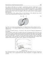
9.2 3D Geometric wide band channel model
The 3D Geometric wide band channel model is presented in Fig.31.
✻
✻
❂ ❂
z
z

x
x

✉
✉
✈
✉
R

x
T
x
✈
✈
✈
✈
✉
✉
✉
✉
✉
✉
✈
✈
✈
✈
✇
✇
✇
✇
✇
✇
A
(1)
Tx
A
(2)
Tx
A

(1)
Rx
A
(2)
Rx
q
R
()
Tx
q
D
()
Rx
C
Rx
()
C
Tx
()
S
(,n)
Rx
S
(,m)
Tx
✙
✉
✾
R
()

Rx
✲
✒
✠
D
()
Tx
✈
✕ v
Rx
✒
v
Tx
✠
❑
α
Rx
▼
α
Tx
✕
❲
θ
(,m)
Tx
✍
❄
θ
(,n)
Rx

✲
y
✒
✲
Fig. 31. 3D Geometric model for MIMO channel (N
R
= 2, N
T
= 2)
Two transmit antennas (A
(1)
Tx
,A
(2)
Tx
) and two receive antennas (A
(1)
Rx
,A
(2)
Rx
) are presented. Wide
band MIMO channel involves several local clusters of scatterers which are distributed around
the transmitter and the receiver. The cluster index is denoted
,  = 1, ,L.Clusteraround
the transmitter C
Tx
() is assumed to be associated with a set of M
()
scatterers (S

(,m)
Tx
; m =
1, ,M
()
). Cluster around the receiver C
Rx
() is assumed to be associated with a set of N
()
scatterers (S
(,n)
Rx
; n = 1, ,N
()
).
We take for notations:
•R
()
Tx
: Transmit cluster radius of index 
•D
()
Tx
: Distance between the reference transmit antenna and the transmit cluster center
• d
1,,m
: Distance between antenna A
(1)
Tx
and a scatterer S

(,m)
Tx
• d
2,,m
: Distance between antenna A
(2)
Tx
and a scatterer S
(,m)
Tx
• d
Tx
: Transmit antennas spacing
•D
Tx↔Rx
: Distance between the transmitter and the receiver
•R
()
Rx
: Cluster radius at the receiver of index 
40
MIMO Systems, Theory and Applications
•D
()
Rx
: Distance between the reference antenna A
(1)
Rx
and the center of the cluster  at the
receiver.

• d
1,,n
: Distance between antenna A
(1)
Rx
and the scatterer S
(,n)
Rx
• d
2,,n
: Distance between antenna A
(2)
Rx
and the scatterer S
(,n)
Rx
The Non-Line of Sight (NLOS) channel coefficients in 3D Geometric model are given by
(Prayongpun, 2009):
h
NLos
qp
(t, f )= lim
M,N→∞
L
∑
=1

PDP()
M
()

N
()
M
()
∑
m=1
N
()
∑
n=1
G
p
(θ
(,m)
Tx
, φ
(,m)
Tx
; β
Tx
, γ
Tx
)a
(p)

m
b
(q)

n

G
q
(θ
(,n)
Rx
, φ
(,n)
Rx
; β
Rx
, γ
Rx
)exp

j

2π( f
(,m)
Tx
+ f
(,n)
Rx
)t + ϕ
mn
+ ϕ
()
0

(89)
• q

∈
{
1, ,N
R
}
• p ∈
{
1, ,N
T
}
• PDP() is the power delay profile which gives the intensity of a signal received through a
multipath channel connecting a pair of clusters.
• G
p
(θ
(,m)
Tx
, φ
(,m)
Tx
; β
Tx
, γ
Tx
) is the gain of antenna p with associated oriented direction
(β
Tx
, γ
Tx
) and a wave propagation direction (θ

(,m)
Tx
, φ
(,m)
Tx
).
• G
q
(θ
(,n)
Rx
, φ
(,n)
Rx
; β
Rx
, γ
Rx
) is the gain of antenna q with associated oriented direction
(β
Rx
, γ
Rx
) and a wave propagation direction (θ
(,n)
Rx
, φ
(,n)
Rx
).

• a
(p)

m
= exp{j2π(p −1)(d
Tx
/λ)[cos(θ
(,m)
Tx
) cos(β
Tx
)+sin(θ
(,m)
Tx
) sin(β
Tx
) cos(φ
(,m)
Tx
−γ
Tx
)]}
• b
(q)

n
= exp{j2π(q −1)(d
Rx
/λ)[cos(θ
(,n)

Rx
) cos(β
Rx
)+sin(θ
(,n)
Rx
) sin(β
Rx
) cos(φ
(,n)
Rx
−γ
Rx
)]}
• f
(,m)
Tx
=(|v
Tx
|/λ) sin(θ
(,m)
Tx
) cos(φ
(,m)
Tx
−α
Tx
)
• f
(,n)

Rx
=(|v
Rx
|/λ) sin(θ
(,n)
Rx
) cos(φ
(,n)
Rx
−α
Rx
)
• ϕ
()
0
= −2π(D
()
Tx
+ D
Tx↔Rx
+ D
()
Rx
)/λ
• ϕ
mn
∼ U[−π, π]
We assume that the transmitter and the receiver have motions above the plan (x, y) with
relative directions α
Tx

and α
Rx
. In 3D Geometric model, the distances are expressed as :
d
1,,m
≈ D
()
Tx
(90)
d
2,,m
≈ D
()
Tx
−d
Tx
cos(θ
(,m)
Tx
) cos(β
Tx
) − d
Tx
sin(θ
(,m)
Tx
) sin(β
Tx
) cos(φ
(,m)

Tx
−γ
Tx
) (91)
d
1,,n
≈ D
()
Rx
(92)
d
2,,n
≈ D
()
Rx
−d
Rx
cos(θ
(,n)
Rx
) cos(β
Rx
) −d
Rx
sin(θ
(,n)
Rx
) sin(β
Rx
) cos(φ

(,n)
Rx
−γ
Rx
) (93)
d
,m,n
≈ D
Tx↔Rx
+ D
()
Rx
sin(θ
(,n)
Rx
) sin(φ
(,n)
Rx
) −D
()
Tx
sin(θ
(,m)
Tx
) sin(φ
(,m)
Tx
) ≈ D
Tx↔Rx
(94)

When there are no scatterers around the transmitter or the receiver, the channel model is
referred as Line of Sight (LOS).
41
Advanced MIMO Techniques: Polarization Diversity and Antenna Selection
9.3 Depolarization phenomena
The polarization of an antenna is defined as the polarization of the wave radiated by the
antenna. At a given position, antenna polarization describes the orientation of the electric
field. Suppose an electromagnetic wave radiated by a transmit antenna has an incident electric
field E
i
with two components E
i,θ
and E
i,φ
. In each scatterer’s environment, the electric field
components are reflected (Fig.32). Reflected elevation and azimuth components of the incident
electric field E
i
are denoted E
r,θ
and E
r,φ
.
q
✕
✼
✲
❥
③
E

i,θ
E
i,φ
E
r,θ
E
r,φ
Fig. 32. Antenna depolarization
The radiation pattern is expressed as a function of the azimuth and elevation amplitudes of
polarization vectors in both the elevation and the azimuth directions (
ˆ
θ and
ˆ
φ).
E
i
= E
i,θ
(θ, φ)
ˆ
θ + E
i,φ
(θ, φ)
ˆ
φ (95)
The reflected electric field is expressed as :
E
r
= SE
i

(96)
where :
• E
r
is the matrix notation for the reflected electric field expressed as:
E
r
=

E
r,θ
E
r,φ

(97)
• S is the scattering matrix given by:
S
=

υ
θθ
υ
θφ
υ
φθ
υ
φφ

(98)
– υ

θθ
and υ
φφ
respectively measure the co-polarization gains relative to the elevation
transmission and the azimuth transmission.
– υ
θφ
measures the depolarization gain of the elevation polarization relative to the
azimuth polarization.
– υ
φθ
measures the depolarization gain of the azimuth polarization relative to the
elevation polarization.
42
MIMO Systems, Theory and Applications
• The matrix notation for the incident electric field is :
E
i
=

E
i,θ
E
i,φ

(99)
The depolarization effect is characterized by the Cross Polarization Discrimination
(XPD)(Raoof & Zhou, 2009)(Raoof & Prayongpun, 2007) which is defined as the power ratio
of the co-polarization and cross-polarization components of the mean incident wave.
The polarization discrimination for the elevation transmission is :

XPD
θ
=
E|υ
θθ
|
2
E|υ
φθ
|
2
(100)
The polarization discrimination for the azimuth transmission is :
XPD
φ
=
E|υ
φφ
|
2
E|υ
θφ
|
2
(101)
Inthefollowing,wedenote:
χ
θ
=
1

XPD
θ
and χ
φ
=
1
XPD
φ
GSCM channel model involving antenna depolarization
The wide band GSCM channel modeling with antenna depolarization is given by :
h
NLOS
qp
(t, f )= lim
M,N→∞
L
∑
=1

PDP()
M
()
N
()
M
()
∑
m=1
N
()

∑
n=1
a
(p)
m
b
(q)
n
exp

j

2π( f
(,m)
Tx
+ f
(,n)
Rx
)t+ϕ
mn
+ϕ

0


G
q,θ
(θ
(,n)
Rx

, φ
(,n)
Rx
; β
Rx
, γ
Rx
)
G
q,φ
(θ
(,n)
Rx
, φ
(,n)
Rx
; β
Rx
, γ
Rx
)

T
S
(,m,n)
Tx,Rx

G
p,θ
(θ

(,m)
Tx
, φ
(,m)
Tx
; β
Tx
, γ
Tx
)
G
p,φ
(θ
(,m)
Tx
, φ
(,m)
Tx
; β
Tx
, γ
Tx
)

(102)
The scattering matrix with the depolarization mechanism is expressed as :
S
(,m,n)
Tx,Rx
=

⎡
⎢
⎢
⎢
⎢
⎣

1
1+χ
(,m,n)
θ
exp

jε
(,m,n)
θθ


χ
(,m,n)
φ
1+χ
(,m,n)
φ
exp

jε
(,m,n)
θφ



χ
(,m,n)
θ
1+χ
(,m,n)
θ
exp

jε
(,m,n)
φθ


1
1+χ
(,m,n)
φ
exp

jε
(,m,n)
φφ

⎤
⎥
⎥
⎥
⎥
⎦

(103)
where ε
(,m,n)
θθ
, ε
(,m,n)
θφ
, ε
(,m,n)
φθ
and ε
(,m,n)
φφ
denote the phase offsets.
9.4 Impact of XPD on system capacity
We examine the impact of the XPD parameter on MIMO system capacity. For the seek of
simplicity, we consider the
(2 × 2) MIMO channel generated according to the Kronecker
channel modeling. The dual polarized MIMO system is adopted (Fig. 33). Assuming that the
CSI is known at the receiver side, the MIMO system capacity can be derived by exploiting the
SVD technique. Fig.34 shows plotted curves of the CCDF for various inverse XPDs and the
curve of the MIMO channel capacity as a function of the XPD. Simulation results show that
43
Advanced MIMO Techniques: Polarization Diversity and Antenna Selection
Rx
1
Tx
1
Rx
2

Tx
2
Transmitter
Receiver
Orthogoanal
antennas
Propagation
Environment
✧
✬✩
✥
✦
✙
✔
✕
✓
✒
✓
✒
☞
✌
✗
✖
✞
✝
☎
✆
✄
✂


✁
✎
✍
✄
✂

✁
Fig. 33. Dual polarized antennas
XPD affects the performances of the MIMO system in terms of the CCDF and the capacity.
The MIMO system capacity is shown to be seriously reduced for high level of the polarization
discrimination. Thus, mismatch in polarization results in losses in the MIMO channel capacity.
0 1 2 3 4 5 6
0
0.1
0.2
0.3
0.4
0.5
0.6
0.7
0.8
0.9
1
Capacity (bits/s/Hz)
P(C> abscisse)


χ = 0.100
χ = 0.300
χ = 0.500

χ = 0.700
χ = 0.900
(a)
1 2 3 4 5 6 7 8 9 10
1.7
1.8
1.9
2
2.1
2.2
2.3
2.4
2.5
XPD
Capacity(bits/s/Hz)
(b)
Fig. 34. Impact of XPD:(a) CCDF for dual polarized MIMO system, (b) Dual polarized MIMO
system capacity
9.5 GSCM channel correlation
Correlation coefficients relative to the NLOS channels h
NLOS
qp
(t, τ) and h
NLOS
˜
q
˜
p
(t, τ) are
expressed as :

R
qp,
˜
q
˜
p
(ξ, τ −τ

)=E[h
qp
(t, τ)h
∗
˜
q
˜
p
(t −ξ, τ

)] (104)
For zero phase offsets and one cluster of scatterers
(L = 1),ifχ
θ
= χ
φ
= χ, then equation
(102) reduces to :
R
qp,
˜
q

˜
p
(ξ)= lim
M,N→∞
1
MN
M
∑
m=1
N
∑
n=1
a
(p)
m
b
(q)
n
a
(
˜
p
)
∗
m
b
(
˜
q
)

∗
n
exp

j

2π( f
(m)
Tx
+ f
(n)
Rx
)

ξ

(105)

G
q,θ
· G
˜
q
,θ
G
q,φ
· G
˜
q,φ


T

1 χ
χ 1

G
p,θ
· G
˜
p
,θ
G
p,φ
· G
˜
p,φ

(106)
44
MIMO Systems, Theory and Applications
The continuous spatial correlation coefficients are given by (Prayongpun, 2009):
R
qp,
˜
q
˜
p
(ξ)=

exp


j
2π
(
˜
p
− p)d
Tx
λ
sin θ
Tx
cos φ
Tx
− j2π f
Tx
ξ sin θ
Tx
cos(φ
Tx
−γ
Tx
)

exp

j
2π
(
˜
q

−q)d
Rx
λ
sin θ
Rx
cos φ
Rx
− j2π f
Rx
ξ sin θ
Rx
cos(φ
Rx
−γ
Rx
)


G
q,θ
· G
˜
q
,θ
G
q,φ
· G
˜
q,φ


T

1 χ
χ 1

G
p,θ
· G
˜
p
,θ
G
p,φ
· G
˜
p,φ

p
(
γ
Tx
)
p
(
γ
Rx
)
p
(
Ω

Tx
)
p
(
Ω
Rx
)
dγ
Tx
dγ
Rx
dΩ
Tx
dΩ
Rx
(107)
• Ω involves the elevation angle and the azimuth angle and dΩ
= sin θdφd θ.
• p
(
Ω
Tx
)
(=
p
(
θ
Tx
, φ
Tx

)
)
and p
(
Ω
Rx
)
(=
p
(
θ
Rx
, φ
Rx
)
)
respectively denote the probability
distribution of the scatterers around the transmitter and the probability distribution of
scatterers around the receiver.
The spatial correlation coefficients R
qp,
˜
q
˜
p
(ξ) is obtained as the product of three terms:
1. Transmit spatial correlation: R
·p,·
˜
p

(ξ)
2. Receive spatial correlation: R
q ·,
˜
q·
(ξ)
3. Polarization correlation: 
where :
R
·p,·
˜
p
(ξ)=


G
p,θ
· G
˜
p,θ
G
p,φ
· G
˜
p,φ

exp
{
j2π(
˜

p
− p)d
Tx
sin θ
Tx
cos φ
Tx
/λ
}
·
exp
{
−
j2π f
Tx
ξ sin θ
Tx
cos(φ
Tx
−γ
Tx
)
}
p
(
γ
Tx
)
p
(

Ω
Tx
)
dγ
Tx
dΩ
Tx
(108)
R
q ·,
˜
q·
(ξ)=


G
q,θ
· G
˜
q,θ
G
q,φ
· G
˜
q,φ

exp
{
j2π(
˜

q
−q)d
Rx
sin θ
Rx
cos φ
Rx
/λ
}
·
exp
{
−
j2π f
Rx
ξ sin θ
Rx
cos(φ
Rx
−γ
Rx
)
}
p
(
γ
Rx
)
p
(

Ω
Rx
)
dγ
Rx
dΩ
Rx
(109)

=

1 χ
χ 1

(110)
In literature, azimuth angles may follow uniform, gaussian, von Mises or Laplacien
distributions. For the elevation angle, three distribution functions can be used which are
uniform , cosinus or gaussian distributions. Depending on the propagation environment, we
should note that both von Mises distribution for the azimuth angle and uniform distribution
for the elevation angle perform better. Thus, azimuth distribution function is expressed as :
p
(φ
Tx
)=
exp
{
k
Tx
cos
(

φ
Tx
−
¯
φ
Tx
)}
2πI
0
(
k
Tx
)
(111)
The elevation distribution function is :
p
(θ
Tx
)=
1
2Δθ
Tx
(112)
where :
• φ
Tx
∈ [−π, π]
45
Advanced MIMO Techniques: Polarization Diversity and Antenna Selection
•

¯
φ
Tx
is the mean azimuth angle
• I
0
(·) is the modified Bessel function of zeroth order
• k
Tx
is a measure of the azimuth angle dispersion. 1/k
Tx
is analogous to the variance in the
uniform distribution.
• Δθ
Tx
is the standard deviation of the Angle spread
• θ
Tx
∈ [
¯
θ
Tx
−Δθ
Tx
,
¯
θ
Tx
+ Δθ
Tx

] where
¯
θ
Tx
is the mean elevation angle
In the following, we present simulation results of the spatial correlation as a function of the
antenna spacing and variable values of the term f
Tx
ξ. We adopt the MIMO system with two
transmit antennas and two receive antennas and we present the plotted curves for the spatial
correlation coefficient relative to the transmit antennas Tx
1
and Tx
2
. Plotted curves for the
spatial correlation are presented in two cases :
1. Single polarized antennas (Fig. 35(a))
2. Dual polarized antennas (Fig. 35(b))
0
0.5
1
1.5
2
2.5
3
0
1
2
3
0

0.2
0.4
0.6
0.8
1
f
Tx
ξ
R
⋅ 1,⋅ 2
d
Tx
/λ
(a)
0
0.5
1
1.5
2
2.5
3
50
100
150
0
0.2
0.4
0.6
0.8
1

φ
mean
f
Tx
ξ
R
⋅ 1, ⋅ 2
(b)
Fig. 35. (a) Spatial correlation for z dipole antennas
(k
Tx
= 50,
¯
φ
Tx
= 90
◦
,
¯
θ
Tx
= 90
◦
, Δθ
Tx
= 90
◦
), (b) Spatial correlation for dual polarized
antennas (z dipole antenna and x dipole
antenna)

(k
Tx
= 50,
¯
φ
Tx
= φ
mean
,
¯
θ
Tx
= 90
◦
, Δθ
Tx
= 90
◦
)
According to Fig. 35(a) and Fig. 35(b), it is obvious that single polarized antennas system
shows less correlation. When dual polarized antennas are deployed, spatial correlation
which is expressed as a function of antenna spacing can be reduced. The impact of dual
polarization depends on the mean azimuth angle
¯
φ
Tx
= φ
mean
and spatial correlation is
shown to be negligible if φ

mean
approaches 90
◦
. Thus, spatial correlation can be nulled by
deploying orthogonal antennas. Finally, we present the impact of dual polarized antennas
on MIMO system capacity. The capacity gain brought by the dual polarized system relative
to the single polarized system is depicted in Fig. 36. The capacity gain that could be
achieved thanks to the use of dual polarized antennas is affected by the mismatch in antenna
polarization. Nevertheless, for low XPDs, the dual polarization scheme considerably improves
the channel capacity when comparing to the single polarized antennas system. Depolarization
phenomena in MIMO system and impact of correlation on MIMO system capacity were
rigorously discussed in references (Raoof & Prayongpun, 2007) and (Raoof & Prayongpun,
2005).
46
MIMO Systems, Theory and Applications
0 0.2 0.4 0.6 0.8 1
0
0.1
0.2
0.3
0.4
0.5
0.6
0.7
0.8
0.9
1
1/XPD
R

.1,.2


−1
−0.5
0
0.5
1
1.5
2
2.5
3
3.5
4
Fig. 36. The capacity gain of (2 ×2) dual polarized antennas
10. RSS based localization in WSN with collaborative sensors
10.1 Scenario description
We propose the scenario depicted in Fig. 37 where two clusters of wireless sensor nodes are
presented. Cluster 1 consists of a source sensor S
Tx
and a set of K sensors which are randomly
distributed in the sensing area.
❞
❢
❢
❡
❢
✕
⑦
③

✯
❣
❣
✲
❣
✿
S
Tx
✈
③
❢
❣
✶
✿
①
S
Rx
✲
D
c
✛
Cluster 1
Cluster 2
Fig. 37. Scenario description
We assume that sensor nodes are equipped with omnidirectional antennas. The source sensor
S
Tx
sends redundant BPSK modulated data signal to the sensor nodes which are located at
Cluster 1. The main problem with the presented scenario is the localization of the sensor S
Rx

.
We adopt the 2D geometrical model. Sensors are distributed in the (x-y) plan and source node
is arbitrary placed at the origin of the system coordinate. The geometric spherical coordinates
are defined by the triplet
(r, θ, φ). Here, θ =
π
2
. The simulated layout for 10 sensors is depicted
in Fig.38. We propose a beamforming based localization algorithm involving Received Signal
Strength (RSS) measurements. We take into assumption that the radius from the origin to S
Rx
is known. Thus, the detection of the target node relies on determining the steering vector that
corresponds to the location of S
Rx
.
47
Advanced MIMO Techniques: Polarization Diversity and Antenna Selection
0 50 100 150
0
50
100
150
x (m)
y (m)
Target
sensor S
Rx
S
Tx
Fig. 38. Network layout (K=10)

10.2 System modeling
The wireless link between sensor S
k
, k = 1, ,K and the target sensor is modeled by LOS
propagation. Each propagation link is characterized by :
1. A Rayleigh distributed attenuation denoted λ
k
.
2. A delay τ
k
relative to the reference sensor S
Tx
:
τ
k
= d
k
·
cos(α
k
)
c
(113)
where :
• d
k
: Distance between sensor k and the source node
• c : Speed of the light
• α
k

: Direction of arrival relative to the target sensor S
Rx
3. A dephasing ψ
k
:
ψ
k
= 2π f
c
·τ
k
(114)
f
c
denotes the frequency carrier.
Each channel gain is therefore expressed as:
h
k
= λ
k
e
jψ
k
; k = 1, ,K (115)
A Hadamard Direct Sequence Code Division Multiple Access (DS-CDMA) code is designed
for redundant transmitted BPSK data spreading. Walsh Hadamard codes are perfectly
orthogonal and employed to avoid interference among users in the propagation link. These
codes are exploited for sensor identification and help to mitigate noise effect. The codes for
users could be expressed as the columns (or the rows) of the Walsh-Hamadard matrix C.The
simplest Hadamard matrix codes are :

C
1
= 1
and
C
2
=

11
1
−1

48
MIMO Systems, Theory and Applications