New Tribological Ways Part 14 docx
Bạn đang xem bản rút gọn của tài liệu. Xem và tải ngay bản đầy đủ của tài liệu tại đây (2.89 MB, 35 trang )
A Novel Tool for Mechanistic Investigation of Boundary Lubrication: Stable Isotopic Tracers
439
Total positive ions m/z 28 (Si
+
)m/z 2 (D
+
)
X
Y
higher
INT ENSIT Y
lower
m/z 318 (OA-D35)
Rubbed area
Fig. 16. Chemical mapping of the C
18
OH + OA-D35 binary film after the tribo-test
By contrast, the binary-component monomolecular film from C
18
OH + OA-D35 provided a
longer lifetime with low friction. Almost no changes in chemical mapping after the tribo-test
for 200 s were observed (Figure 16). The results indicate that the C
18
OH + OA-D35 binary
film remained on the surface even after the tribo-test. In consequence, the tribological
properties of the binary-component monomolecular film are in good agreement with the
results of SIMS analysis.
An interaction between C
18
NH
2
and OA-D35 through the ionic interactions is possible. This
makes the adsorption force of OA-D35 on the Si surface, which retards the durability of the
film. On the other hand, an interaction of C
18
OH with OA-D35 is possible through hydrogen
bonding between the polar functional groups, alcohol, and carboxyl group. It should be
noted that the hydrogen bond is much weaker than the ionic bond. Therefore, the
adsorption force of OA-D35 was not weakened by the presence of C
18
OH, which,
advantageously, seems to form certain mobile phases on the surface.
2.4 Lubrication mechanism of diamond-like carbon coatings with water [17-18]
Diamond-like carbon (DLC) coatings on metallic materials possess many advantages to
tribo-materials such as corrosion resistance, wear resistance, and friction reduction [19]. One
of the features of using a DLC coating as a tribo-material is its applicability in humid
environments or in water [20]. Furthermore, it has been reported that water improves the
tribological properties of DLC. Although the formation of a boundary film by the tribo-
chemical reaction of water with DLC has been suggested, a mechanistic investigation based
New Tribological Ways
440
on surface chemistry is difficult. The tribo-chemical reaction of water is supposed to provide
hydrogen or oxygen to DLC surfaces. Besides water as lubricating fluid, there are other
sources of hydrogen and oxygen atoms under tribological conditions. Examples include
oxygen in air or metal oxides, hydrogen in organic contaminants, or DLC itself. Resources of
hydrogen or oxygen could not be identified by the usual procedure, even if increments of
these elements on surfaces were detected after rubbing. The stable isotopic tracer technique
is expected to be powerful tool in studying the tribo-chemistry of DLC. Heavy water, such
as D
2
O and H
2
18
O were employed in this work. DLC coatings were deposited on the silicon
surface by a thermal electron excited chemical vapor deposition procedure using toluene as
carbon source. The resultant material was slid against a SUS 440C (JIS) stainless steel ball at
a load of 10 N under a reciprocating motion at the frequency of 1 Hz. The three lubricants,
H
2
O, D
2
O, H
2
18
O provided similar tribological properties, as shown in Figure 17.
0.00
0.05
0.10
0.15
0.20
0 102030405060
Friction coefficient, -
Test duration, min
H
2
O
D
2
O
H
2
18
O
Fig. 17. Friction trace during the tribo-test with water or heavy water
Chemical mapping of the DLC surfaces obtained by SIMS analysis shows a remarkable
increase in deuterium content on the rubbed surface with D
2
O (Figure 18). Careful analysis
of the mapping indicates the deuterium is bonded to oxygen (OD, m/z at 17) and to carbon
(CD, m/z at 14). It should be noted that the fragment ion of m/z 14 could be identified as
the CD moiety or CH
2
moiety. Presence of the former was supported by another
considerable fragment ion of m/z 2, which corresponds to D. An increase in
18
O on the
surfaces rubbed with H
2
18
O also supports the tribo-chemical reaction of water with DLC. A
considerable increase in the fragment ions of m/z 18 and m/z 19, which corresponded to
18
O and
18
OH, respectively, indicates the formation of a new carbon-oxygen bond. It should
be noted that the contents of
16
O (regular oxygen) outside the worn surface is higher than
that inside worn surface. The results suggest that
16
O-containing compounds that existed on
A Novel Tool for Mechanistic Investigation of Boundary Lubrication: Stable Isotopic Tracers
441
nonrubbed surfaces were worn off under the tribological conditions. However,
identification of the
16
O-containing compound(s) on nonrubbed surface was difficult by the
SIMS analysis.
On the basis of SIMS analysis, we wish to propose the mechanism of tribo-chemical reaction
of water with DLC as expressed in Figure 19. Both homolysis and heterolysis are possible as
the initial step of the reaction when DLC was exposed to mechanical stress. The former
yields carbon radicals and the latter yields carbocations and carbanions as active
intermediates. Then heavy water reacts with the active intermediates and results in the
formation of new C–D and C–OD bonds. In summary, clear evidence of the tribo-chemical
reaction of water with DLC was observed using two isotopic tracers, deuterium and
18
O.
2.5 Lubrication mechanism of organic friction modifier additives in hydrocarbon oils
[21]
GMO (Glycerol monooleate, 2,3-dihydroxypropyl 9(Z)-octadecenoate) is known as one of
the organic friction modifiers that improves the tribological properties of hydrocarbon oils.
In fact, a solution of GMO in PAO (poly-alpha-olefin) dramatically reduced the friction of
steel-DLC [22]. An XPS analysis of the rubbed surface with GMO-PAO indicated the
presence of carbonyl compounds on the surface [23]. The results suggest that adsorption of
GMO yielded the boundary film on the surface, thereby improving the tribological
properties. However, the chemical resolution of XPS analysis for carbon is not sufficient for
further investigations. There are two possibilities for the structure of the boundary film. One
is an adsorption film of GMO itself and the other is an adsorption film of oleic acid, which is
produced by the decomposition of GMO under the tribological conditions. It is difficult to
distinguish between GMO and carboxylic acid by their chemical shifts of the carbonyl
group.
m/z 14 (CD)
H
2
O
D
2
O
m/z 18 (OD)
m/z 2 (D)
m/z 16 (O)
m/z 17 (OH)
m/z 17 (OH)m/z 16 (O)
m/z 17 (OH) m/z 18 (
18
O) m/z 19 (
18
OH)
m/z 16 (O)
H
2
18
O
inside
(rubbed
surface)
outside
Fig. 18. Chemical mapping of DLC surface after tribo-test with water
New Tribological Ways
442
C
C
D
C
C
D
O
C
DC
O
D
C
C
Mechanical
stress
homolysis
heterolysis
C
C
D
C
C
D
O
C
DC
O
D
COD
DC
+
Carbon radicals
Carbocation
and carbanion
Fig. 19. Reaction mechanism of water with DLC surface under the tribological conditions
There are other ways in which carbonyl compounds are produced on the rubbed surface. An
auto-oxidation of hydrocarbons usually occurs during the tribo-test under air. The reaction
yields various organic oxides including carbonyl compounds. More troublesome, organic
contaminants including carbonyl compounds exist everywhere. Therefore, it is difficult to
eliminate carbonyl compounds derived not from GMO, but from sources other than GMO.
The present stable isotopic tracer technique would clarify all of these problems. For this
purpose, perdeuterio-GMO (in which all hydrogen atoms in GMO are substituted with
deuterium) was desired. However, preparation of perdeuterio-GMO seemed difficult
because of the availability of its precursors. Generally, GMO is prepared by the esterification
of 9(Z)-octadecenoic acid (oleic acid) with propane-1,2,3-triol (glycerol). Commercially
available precursors for isotope labeled GMO (where at least one atom is substituted by D or
13
C) are listed in Figure 20. Due to limitations in the available precursors, we were required
to design isotopic labeled GMO that makes SIMS analysis effective. For this purpose, the
fragmentation of GMO in SIMS analysis was considered carefully. GMO has two moieties:
an alcoholic moiety with three carbons and the carbonyl moiety with 18 carbons. One of the
major fragmentations of GMO is the scission of the ester bond, dividing GMO into a three-
carbon moiety and 18-carbon moiety. To identify both fragments as fingerprint fragments in
SIMS analysis, we have selected two precursors. One is tri-
13
C-propane-1,2,3-triol and the
other is 1-
13
C-9(Z)-octadecenoic acid. It should be noted that the former produces the three-
carbon fragment with increments of m/z 3 from the natural (unlabeled) propane-1,2,3-triol.
The latter produces the 18-carbon fragment with increments of m/z 1 from the natural 9(Z)-
octadecenoic acid. In this manner two labeled-GMOs, namely c-GMO and g-GMO, were
prepared (Figure 21).
A Novel Tool for Mechanistic Investigation of Boundary Lubrication: Stable Isotopic Tracers
443
m/z 93
HO OH
OH
*
m/z 94
HO OH
OH
**
m/z 95
HO OH
OH
*
**
m/z 95
DO OD
OD
m/z 95
HO OH
OH
m/z 98
DO OD
OD
D
D
D D
D
D
HO
O
m/z 285
*
HO
O
m
/
z285
*
HO
O
m/z 286
HO
O
m
/
z286
D D
D
D
where * means
13
C
Fig. 20. List of commercially available 9(Z)-octadecenoic acid and propane-1,2,3-triol labeled
with stable isotope(s)
*
*
*
*
whe
r
e * means
13
C
g-GMO m=359
O
O
OH
OH
c-GMO m=357
O
O
OH
OH
GMO m=356
O
O
OH
OH
Fig. 21. Structure of labeled GMO as a model additive
We acquired mass spectra of GMOs on nonrubbed surfaces to find out their "fingerprint"
fragment ions. GMO yielded fragment ions at m/z 265 and 339 in positive ion spectra and at
m/z 280 in negative ion spectra. c-GMO and g-GMO gave fragment ions according to their
number of
13
C. These fragment ions were generated by scission of the carbon-oxygen bond
New Tribological Ways
444
in the additive molecule. Here we paid attention to the following fragments of GMO to
investigate the boundary film formed on the rubbed surfaces (Figure 22).
“Fragment-A” as the acyl moiety
“Fragment-C” as the carboxyl moiety
“Fragment-E” as an ester dehydroxylated from the original molecule
Fragment A: m = 265 for GMO and g-GMO, m = 266 for c-GM O
Fragment C: m = 281 for GMO and g-GMO, m = 282 for c-GM O
Fragment E: m = 339 for GMO, m = 340 for c-GMO, m = 342 for g-GMO
Original : m = 356 for GMO, m = 357 for c-GMO, m = 359 for g-GMO
O
O
OH
OH
Fig. 22. Formula weight of the fragment ions from GMOs
2.6 SIMS analysis of GMO on DLC
Three GMOs were dissolved in PAO and the solutions were employed for the tribo-test. All
GMOs provided similar tribological properties, as shown in Figure 23. The results indicate
there are no effects on isotope(s) on the tribological properties, which is essential in the use
of an isotope-labeled molecule for chemical analysis.
0.00
0.05
0.10
0.15
Additive-free GMO c-GMO g-GMO
Friction coefficient, -
Additive
Fig. 23. Results of the tribo-test using labeled GMO in PAO
A Novel Tool for Mechanistic Investigation of Boundary Lubrication: Stable Isotopic Tracers
445
“Fragment-A” and “Fragment-E” were found in the positive mass spectra, and “Fragment-
C” was found in the negative mass spectra of the rubbed surfaces (Figures 24-25). The
hydrolysis of GMO yields 9Z-octadecenoic acid (oleic acid), which may adsorb on DLC
surfaces. We confirmed analytically whether or not the acid exists on the surfaces. GMO and
9Z-octadecenoic acid afford "Fragment-A" and "Fragment-C." Obviously, “Fragment-E” is
attributed to GMO. We compared the relative intensity of (Fragment-A)/(Fragment-E). Our
hypothesis is as follows; if the relative intensity of the acid on the wear track is higher than
that on the nonrubbed surface, then the acid exists on the rubbed surface. We found the
same relative intensities of the fragments. Therefore, the boundary film is mainly composed
of GMO as an ester, and if at all, adsorption from the acid constitutes a minor portion. These
results indicate that hydroxyl group in GMO is an anchor for interactions with the DLC
surfaces.
Finally, we wish to propose the contents of the boundary film that provide low friction upon
steel-DLC contact. Adsorption of GMO on the rubbed and on the nonrubbed DLC was
detected by SIMS analysis. It has been reported that rubbing can activate DLC surfaces,
which result in the adsorption of additives [24, 20]. However, we could not find any clear
2
00 250 300 350
0
50
100
150
200
250
300
Total C ounts (0.18 amu bin)
Integral: 11850 4UNSAVED + Ions 173µm 876417 cts
243
225
253219
207
335
279
202
211
239
339
265
2
00 250 300 350
0
100
200
300
400
500
Total Counts (0.18 amu bin)
Integral: 22294 5UNSAVED + Ions 173µm 1033335 cts
252
336
215 226
207
219
279 380
202
239
266
340
2
00 250 300 350
0
200
400
600
800
1000
1200
1400
Total C ounts (0.18 amu bin)
Integral: 133218 10UNSAVED + Ions 173µm 2244517 cts
252
227
215
279
342
219
370
313
202
239
265
388
rubbed with
c-GMO in PAO
rubbed with
g-GMO in PAO
rubbed with
GMO in PAO
m/z 265
m/z 339
m/z 266
m/z 265
m/z 342
m/z 340
Fig. 24. Mass spectrum of wear track rubbed with GMOs (m/z 200–400, positive)
New Tribological Ways
446
2
00 250 300 350
0
2000
4000
6000
8000
Total C ounts (0.18 amu bin)
Integral: 38868 6UNSAVED - Ions 173µm 3173379 cts
227
255
281
2
00 250 300 350
0
5000
10000
15000
Total C ounts (0.18 amu bin)
Integral: 58955 7UNSAVED - Ions 173µm 3923342 cts
282
2
00 250 300 350
0
5000
10000
15000
20000
25000
30000
35000
Total C ounts (0.18 amu bin)
Integral: 170786 13UNSAVED - Ions 173µm 7020437 cts
281
rubbed with
c-GMO in PAO
rubbed with
g-GMO in PAO
rubbed with
GMO in PAO
m/z 281
m/z 281
m/z 282
Fig. 25. Mass spectrum of wear track rubbed with GMOs (m/z 200–400, negative)
evidence for the activation of surfaces by rubbing, if the intensities of GMO on the rubbed
surfaces were compared with those on the nonrubbed surfaces. Aside from "Fragment-A"
and "Fragment E," several broad peaks were found in the mass spectrum. Careful analysis of
the spectrum revealed that the cycle of the broad peaks is approximately m/z 14, indicating
a methylene (CH
2
, m/z 14) unit exists on DLC surfaces. The fragment ions are likely
attributed to PAO, which is the major component of the system. A liquid clathrate-type
boundary film (which involves an insertion of a branched hydrocarbon moiety in PAO into
the adsorption film of GMO) was suggested [21].
3. Scope and limitations
In this article, we introduced a new technique for the investigation of tribo-chemistry that is
based on stable isotopic tracers. The potential applicability of this technique would include
the following three categories.
1. Degradation of preformed boundary film: Examples include monomolecular film; self-
assembled mono-layers (SAMs); and any other surface treatment, including coatings.
A Novel Tool for Mechanistic Investigation of Boundary Lubrication: Stable Isotopic Tracers
447
For this purpose, isotope-labeled compounds can be employed as precursors of surface
treatment.
2. The interaction of additives on the rubbed surface: The results of the binary-component
monomolecular film can be applied to study synergism or antagonism for each additive
in multicomponent lubricants.
3. Tribo-chemical reaction of base fluids with the surfaces of materials: Simple chemicals
in the chemical structure, such as water, are applicable for this purpose at present. The
main difficulties lie in availability of isotope-labeled base fluids.
4. The interaction of additive molecules with tribological surfaces: This is still an emerging
technique for tracing the target molecule (usually tribo-improving additive) after the
tribological process. The most challenging aspect of this technique is to detect small
quantities of isotope(s) present in the system. For example, the solution of c-GMO in
PAO contains approximately 0.04% of the labeled
13
C compared to the total number of
carbons in the solution. Note that
13
C yields a fragment ion of m/z 13, which is the
same m/z as
12
CH from hydrocarbons. If a considerable amount of
13
C exists in the
system, the intensity of the fragment ion at m/z 13 should be obviously increased. The
detection of these small quantities of isotopes is difficult. We have solved this problem
by tracing major fragment ions derived from two or three precursors. This requires well
designed model molecules based on the fragmentation of molecules during SIMS
analysis. The introduction of the stable isotope(s) into the appropriate position in the
molecule is essential.
It should be pointed out that the stable isotopic technique is highly suitable for organic
compounds comprised of only hydrogen and carbon, and possibly also those containing
oxygen and/or nitrogen atoms. For these organic compounds, the conventional surface
analyses for tribology such as AES, EPMA, and XPS do not provide sufficient chemical
resolution. Therefore, it is usually difficult to distinguish between the target molecule and
organic contaminants. Usually there are small quantities of the target molecule on the
rubbed surface. This makes the surface analysis more difficult. On the other hand, most
tribo-active elements in lubricants, such as phosphorus, sulfur, molybdenum, zinc, and
chlorine are well identified by the conventional surface analyses in tribology. Although AES,
EPMA, and XPS can well detect the heavy elements with high sensitivity, they do not or
hardly detect the light elements such as hydrogen and carbon. SIMS detects all elements if
they are effectively ionized.
SIMS is a surface sensitive analysis whose analytical depth is as thin as 1–2 nm. Therefore,
the sample should contain smooth surfaces to obtain optimal analytical results. The
tribological process usually results in surfaces with submicrometer asperities even under a
mild wear regime. The present work was achieved by employing wear resistance materials
such as DLC. SIMS analysis was performed before wear occurs. This implies the technique is
limited to mixed lubrication under low wear conditions. The placement of D,
13
C, or
18
O
enriched atoms at the appropriate position(s) in the molecule is not always available at a
reasonable cost. Therefore, isotope-labeled molecule should be designed based on their
fragmentation during SIMS analysis.
SIMS approaches in tribo-chemistry using nonlabeled additives have been also achieved by
detecting molecular ions or quasi-molecular ions [25-29]. However, signals corresponding to
New Tribological Ways
448
the target molecule are weak. Our isotope labeled approach usually provides clear signals
with detailed analysis of the boundary film. In addition to these advantages of SIMS, the
combination of multiple analytical tools is highly recommended for studying tribo-
chemistry [30-31].
4. References
[1] Pawlak, Z. (2003): Tribochemistry of Lubricating Oils. Elsevier B.V., Amsterdam.
[2] Allum, K.G.; Forbes, E.S. (1968): The Load-carrying Mechanism of Organic Sulphur
Compounds. Application of Electron Probe Microanalysis . ASLE Transactions 11 2:
162-175.
[3] Buckley, D.H.; Pepper, St.V. (1972): Elemental Analysis of a Friction and Wear Surface
During Sliding Using Auger Spectroscopy . ASLE Transactions 15 4: 252-260.
[4] Moulder, J.F.; Stickle, W.F.; Sobol, P.F.; Bomben, K.D. (1995): Handbook of X-Ray
Photoelectron Spectroscopy. Edited by Chastain, J.; King, R.C.Jr. ULVAC-PHI, Inc.,
Chigasaki, Japan.
[5] Kasrai, M.; Cutler, J.N.; Gore, K.; Canning, G.; Bancroft, G.M.; Tan, K.H. (1998): The
Chemistry of Antiwear Films Generated by the Combination of ZDP and MoDTC
Examined by X-ray Absorption Spectroscopy. Tribology Transactions 41 1: 69-77.
[6] Benninghoven, A.; Hagenhoff, B.; Niehuis E. (1993): Surface MS: probing real-world
samples. Analytical Chemistry 65 14: 630-640.
[7] Vickerman, J.C.; Gilmore, I.S. Surface Analysis - The Principal Techniques, 2nd Edition
(2009): John Wiley and Sons, West Sussex.
[8] Criss, R.E. (1999): Principles of Stable Isotope Distribution. Oxford University Press,
New York.
[9] Sakurai, T.; Ikeda, S.; Okabe, H. (1962): The Mechanism of Reaction of Sulfur Compounds
with Steel Surface During Boundary Lubrication, Using S35 as a Tracer. ASLE
Transactions 5 1: 67-74.
[10] Vickerman, J.C.; Briggs, D; Henderson, A. (2007): Static SIMS Library, 4th edition.
SurfaceSpectra Ltd. Manchester.
[11] Minami, I.; Kubo, T.; Fujiwara, S.; Ogasawara, Y.; Nanao, H.; Mori, S. (2005):
Investigation of tribo-chemistry by means of stable isotopic tracers; TOF-SIMS
analysis of Langmuir-Blodgett films and examination of their tribological
properties. Tribology Letters 20 3/4: 287-297.
[12] Bowden, F. P.; Tabor, D. (2001): The Friction and Lubrication of Solids. Oxford
University Press, New York.
[13] Novotny, V.; Swalen, J.D.; Rabe, J.P. (1989): Tribology of Langmuir-Blodgett Layers.
Langmuir 5 2: 485-489.
[14] Nutting, G.C., Harkins, W.D. (1939): Pressure-Area relations of Fatty Acid and Alcohol
Monolayers. Journal of American Chemical Society 61 : 1180-1187.
[15] Minami, I.; Furesawa, T.; Kubo, T.; Nanao, H.; Mori, S. (2008): Investigation of tribo-
chemistry by means of stable isotopic tracers: Mechanism for durability of
monomolecular boundary film. Tribology International 41 11: 1056-1062.
A Novel Tool for Mechanistic Investigation of Boundary Lubrication: Stable Isotopic Tracers
449
[16] Dominguez, D.D.; Mowery, R.L.; Turner, N.H. (1994): Friction and Durabilities of Well-
Orderd, Close-Packed Carboxylic Acid Monolayers Deposited on Glass and Steel
Surfaces by the Langmurir-Blodgett Technique. Tribology Transactions 37 1: 59-66.
[17] Wu, X.; Ohana, T.; Tanaka, A.; Kubo, T.; Nanao, H.; Minami, I.; Mori, S. (2007):
Tribochemical investigation of DLC coating tested against steel in water using a
stable isotopic tracer. Diamond and Related Materials 16 9: 1760-1764.
[18] Wu, X.; Ohana, T.; Tanaka, A.; Kubo, T.; Nanao, H.; Minami, I.; Mori, S. (2008):
Tribochemical investigation of DLC coating in water using stable isotopic tracers.
Applied Surface Science 254 11: 3397-3402.
[19] Miyoshi, K.; Street, K.W.Jr. (2004): Novel carbons in tribology. Tribology International
37: 865-868.
[20] Li, H.; Xu, T.; Wang, C.; Chen, J.; Zhou, H.; Liu, H. (2005): Tribochemical effects on the
friction and wear behaviors of diamond-like carbon film under high relative
humidity condition. Tribology Letters 19 3: 231-238.
[21] Minami, I.; Kubo, T.; Nanao, H.; Mori, S.; Okuda, S.; Sagawa, T. (2007): Investigation of
Tribo-Chemistry by Means of Stable Isotopic Tracers, Part 2: Lubrication
Mechanism of Friction Modifiers on Diamond-Like Carbon. Tribology Transactions
50 4: 477-487.
[22] Kano, M. (2006): Super low friction of DLC applied to engine cam follower lubricated
with ester-containing oil. Tribology International 39: 1682-1685.
[23] Ye, J.; Okamoto, Y.; Yasuda, Y. (2008): Direct Insight into Near-frictionless Behavior
Displayed by Diamond-like Carbon Coatings in Lubricants. Tribology Letters 29 1:
53-56.
[24] Kano, M.; Yasuda, Y.; Okamoto, Y.; Mabuchi, Y.; Hamada, T.; Ueno, T.; Ye, J.; Konishi,
S.; Takeshima, S.; Martin, J.M.; Bouchet, M.I. De Barros; Le Mogne, T. (2005):
Ultralow friction of DLC in presence of glycerol mono-oleate (GMO). Tribology
Letters 18 2: 245-251.
[25] Dauchot, G.; Castro, E. De; Repoux, M.; Combarieu, R.; Montmitonnet, P.; Delamare, F.
(2006): Application of ToF-SIMS surface analysis to tribochemistry in metal forming
processes. Wear 260: 296-304.
[26] Wiltord, F.; Martin, J.M.; Le Mogne, T.; Jarnias, F.; Querry, M.; Vergne, P. (2006):
Reaction mechanisms of alcohols on aluminum surfaces. Tribologia 37 6: 7-20.
[27] Tohyama, M.; Ohmori, T.; Murase, A. Masuko, M. (2009): Friction reducing effect of
multiply adsorptive organic polymer. Tribology International 42 6: 926-933.
[28] Gunsta, U.; Zabelb, W. R.; Vallec, N.; Migeonc, H N.; Pollb, G.; Arlinghausa, H.F.
(2010): Investigation of laminated fabric cages used in rolling bearings by ToF-
SIMS. Tribology International 43 5-6: 1005-1011.
[29] Reichelt, M.; Gunst, U.; Wolf, T.; Mayer, J.; Arlinghaus, H.F.; Gold, P.W. (2010):
Nanoindentation, TEM and ToF-SIMS studies of the tribological layer system of
cylindrical roller thrust bearings lubricated with different oil additive formulations.
Wear 268 11-12: 1205-1213.
[30] Georges, J.M.; Martin, J.M.; Mathia, T.; Kapsa, P.H.; Meille, G.; Montes, H. (1979):
Mechanism of boundary lubrication with zinc dithiophosphate. Wear 53 1: 9-34.
New Tribological Ways
450
[31] Minfray, C.; Martin, J.M.; Esnouf, C.; Le Mogne, T.; Kersting, R.; Hagenhoff, B. (2004): A
multi-technique approach of tribofilm characterization. Thin Solid Films 447-448:
272-277.
22
FEM Applied to Hydrodynamic Bearing Design
Fabrizio Stefani
University of Genoa
Department of Mechanics and Machine Design
Italy
1. Introduction
Nowadays hydrodynamic lubrication analysis involves sophisticated models that use a
large number of variables. For instance the evaluation of temperatures, which directly
determine the viscosity of the lubricant fluid and hence its load carrying capacity, has
become a standard procedure and the related analysis type is referred to as
ThermoHydroDynamic (THD) analysis. ThermoElastoHydroDynamic (TEHD) models introduce
a further enhancement in lubrication analysis by including the simulation of bearing
deformations due to mechanical loads and/or thermal effects.
TEHD lubrication is an interdisciplinary field including structural, thermal, thermo-elastic
and hydrodynamic simulations. Hence it requires a multi-physic approach that should be
based on a well-rounded discretization technique capable of simplifying the simultaneous
management of different interconnected models, which must exchange data between
themselves. This task is well-accomplished by the Finite-Element Method (FEM), an overall
discretization technique particularly suited for problems with complicated integration
domains and non-smooth solutions.
A TEHD model of a kinematic pair simulates the thermal and mechanic interaction among
the lubricant film and the lubricated solid members. As far as the fluid film sub-model is
concerned, it must rely on the mass and energy conservation principles. The separation of
the fluid (cavitation) in the divergent film region and the presence of feed grooves on
bearing surfaces encumber the formulation of the conservation principles especially in the
finite-element perspective and require special modelling techniques.
The present chapter is aimed to provide the theoretical foundation of FEM mass- and
energy-conserving models as well as to report their application to the THD and/or TEHD
analysis of different bearing types. Author’s original contributions to the simulation
methods are explained. They include the FEM groove-mixing theory, the SUPG stabilization
of the conservation equations and the "quasi-3D" approach to the thermal problem. The
theoretical construct is useful to enable the analysts to manage the models and to
understand the responses. The application examples are relevant to both journal and axial
bearings with fixed and tilting pads, in order to demonstrate the high flexibility of the
method. With few modifications the presented method can be applied to the design of
several types of bearings in both steady and dynamic loading conditions. The scope of the
paper is anyway limited to the analysis of steadily-loaded bearings working in laminar
lubrication regime.
New Tribological Ways
452
2. State-of-the-art
Modern lubrication analysis methods enable us to assess bearing performances with high
accuracy. By taking advantage of detailed THD simulations the maximum deviation
between experimental findings and numerical predictions for white metal temperatures
may be less than 3-4°C (Banwait & Chandrawat, 1998).
TEHD analysis is compulsory in order to achieve sufficiently reliable results for highly
loaded journal bearings (Bouyer & Fillon, 2004), tilting pad journal bearings (Chang et al.,
2002), thrust bearings (Brugier & Pasal, 1989) and dynamically loaded supports (i.e. big end
bearings of connecting rods for automotive engines) (Piffeteau et al., 2000). TEHD analysis
may also be convenient in the case of journal bearings with stiff housing (i.e. for
turbomachineries) in order to avoid assumptions about the effective clearance in working
conditions.
FEM is more and more often used in lubrication analysis (Booker & Huebner, 1972; Bonneau
& Hajjam, 2001). A FEM version of the classic groove-mixing theory (Robinson & Cameron,
1975) is explained in the following. It has been developed by formulating the energy balance
for the supply grooves at the element level, in order to deal with all of the lubrication
problem details in finite-element terms.
Suitable stabilization techniques are compulsory in lubrication analysis to solve by means of
FEM the energy and the cavitation equations, whereas they rule parabolic and hyperbolic
differential problems, respectively. The Streamline Upwind Petrov-Galerkin (SUPG)
technique (Kelly et al., 1980; Tezduyar & Sunil, 2003), applied by the author to both
problems, is fully explained in the following. Although more straightforward upwinding
techniques have been initially proposed by other authors (Kumar & Booker, 1991), SUPG is
more general, as it does not depend on the element type.
As convection is the main mechanism of heat exchange in the lubricant film, oil
temperatures and flows are directly related. Hence a consistent treatment of the thermal
problem demands an equally reliable model of film hydrodynamics.
In this perspective the FEM mass-conserving algorithms developed in the last decade by
researchers (Kumar & Booker, 1991; Bonneau & Hajjam, 2001) are an essential tool to
provide the accurate estimate of the lubricant flow needed by THD and TEHD analysis
methods. A mass- and energy-conserving FEM model has been presented by Kumar &
Booker (1994). The resulting algorithm is fast as it turns the three-dimensional (3D) thermal
problem in a two-dimensional (2D) one by solving the energy equation averaged across the
film thickness and by assuming adiabatic walls. Afterwards such a method has been
enhanced in a previous work (Stefani & Rebora, 2009), where it is incorporated in a
complete 3D TEHD simulation and it is completed with boundary conditions consistent
with the continuity of mass and energy throughout the integration domain.
To this purpose the temperature variation across the film thickness is calculated by fitting
the temperature profile with a fourth-order polynomial (quasi-3D approach) and the above-
mentioned groove-mixing theory is employed. In such an arrangement the algorithm has
shown good agreement with experimental results. The computational cost is still reasonable
and the algorithm is very flexible and well-suited to different bearing types and geometries.
Consequently the model can serve as the basis for codes dedicated to bearing design and
verification for industrial purposes.
FEM Applied to Hydrodynamic Bearing Design
453
3. Basic equations
3.1 Thin film mechanics equations
In kinematic pairs working in hydrodynamic and elastohydrodynamic lubrication regime,
the lubricant action is exerted through a thin film between two members (with facing
surfaces 0 and 1) in motion at velocity V
0
and V
1
, respectively (Fig. 1).
The following usual "Reynolds hypotheses" are assumed. The lubricant is Newtonian and it
flows in laminar regime in the narrow clearance between the two members, with no-slip
conditions at the walls. The film curvature yields negligible effects.
Fig. 1. Reference system O(x, y, z) and flow between the two surfaces 0 and 1 moving with
velocity V
0
={U
0
, V
0
, 0} and V
1
={U
1
, V
1
, 0}
The velocity distributions of the fluid into the film thickness can be obtained from the Navier-
Stokes equations, simplified by means of the above-mentioned assumptions and integrated
with suitable boundary conditions (the fluid velocity at the surfaces 0 and 1 are V
0
and V
1
,
respectively). After velocity is substituted in the continuity equation, its integration in a
columnar element of fluid (Fig. 1) with height H = H
1
– H
0
and rectangular basis dx · dz
provides the thin film mechanics equation, also referred to as Reynolds generalized equation,
(Dowson, 1967). At time t, for a full film of compressible fluid developed in a rectangular
domain, where a cartesian coordinate system O(x, y, z) is fixed, it states
()
{}
()
11 00 1 0
pp
gg UHUHfUUH
xxzzx t
ρρρ ρ
∂∂
∂∂∂ ∂
⎛⎞⎛⎞
⎡⎤
+ = −−−+
⎜⎟⎜⎟
⎣⎦
∂∂∂∂∂ ∂
⎝⎠⎝⎠
(1)
where the hydrodynamic pressure p as well as the fluid density ρ are independent of the y
coordinate and
10
2
21 0
/
/
fii
gi i i
=
⎫
⎪
⎬
=−
⎪
⎭
(2)
with
1
0
s
H
s
H
y
idy
μ
=
∫
(3)
New Tribological Ways
454
The lubricant viscosity μ (eq. (3)) is variable along the film thickness (with the y coordinate)
as well as in the bearing surface (with the x and z coordinates).
Although equation (1) is time dependent, it is not referred to as the equation of the thin film
dynamics, as inertia and volume forces are negligible in a thin film. Hence the reference
frame O(x, y, z) can be chosen regardless of whether it is inertial or not.
In order to express eq. (1) in a form useful for bearing analysis, the plane y=0 is assumed to
lie on the surface 0. Therefore equations of surfaces 0 and 1 become H
0
= 0 and H
1
= H,
respectively. In addition, let O(x, y, z) be fixed to surface 0, namely surface 0 is steady in this
reference frame. Hence, if U is the relative velocity between surface 1 and surface 0, the
kinematic terms in eq. (1) are U
0
=0 and U
1
=U.
These assumptions simplify the thin film mechanics equation as follows
()
()
pp
gg
UH
f
H
xxzzx t
ρρρ ρ
∂
∂
∂
∂∂ ∂
⎛⎞⎛⎞
⎡⎤
+=−+
⎜⎟⎜⎟
⎣⎦
∂∂∂∂∂ ∂
⎝⎠⎝⎠
(4)
Equation (4) may be used for analysis of journal bearings, when their geometry and
operating conditions enable Reynolds hypotheses to be fulfilled. As curvature effects are
neglected the x axis is set in circumferential direction (x = R
ϑ, where R is the shaft radius).
In order to avoid the simulation of moving grooves, the surface where feed holes and/or
lubricant supply grooves are machined is chosen as surface 0. Usually surface 0 and surface
1 lie on the bush and the journal respectively, as in the case of rotor journal bearings,
submitted to steady loads and fed through suitable grooves in the bushing. In big end
bearings of connecting rods for internal combustion engines, working under dynamic loads,
the feed holes are machined in the crankshaft. Hence the sleeve wall may be chosen as
surface 0 only if it houses a circumferential groove. Otherwise surface 0 is chosen on the
journal, and U becomes the velocity of the bearing with respect to the journal. Nevertheless,
as this chapter focus more specifically on rotor bearings, the reference surface 0 for radial
bearings will be always on the sleeve in the following. Consequently, if
ω is the shaft
rotation speed (with respect to the bearing), U =
ω R.
The relative surface velocity U (or
ω) may either depend or not depend on the x (or ϑ)
coordinate as for journal bearings submitted to either dynamic or steady loads, respectively.
In the former case such a dependency yields higher order infinitesimal in eq. (4) and it can
be neglected in the simulation of the thin film mechanics.
The resulting form of the thin film mechanics equation for journal bearings is
()
()
2
1
pp
gg
H
f
H
zz t
R
ρρωρ ρ
ϑϑ ϑ
∂
∂
∂
∂∂ ∂
⎛⎞⎛⎞
⎡⎤
+=−+
⎜⎟⎜⎟
⎣⎦
∂∂∂∂ ∂ ∂
⎝⎠⎝⎠
(5)
In the annular domain, where the lubricant film develops in the case of thrust bearings, the
coordinate frame used to locate a generic point Q (Fig. 3) is the cylindrical coordinate system
O(r, y, ϑ). An analogous integration of the Navier-Stokes and continuity equations in the
reference frame O(r, y, ϑ), leads to
()
()
11
gp p
g
rH
f
H
rr rr r t
ρ
ρωρ ρ
ϑϑ ϑ
∂∂
∂∂ ∂ ∂
⎛⎞⎛⎞
⎡⎤
+=−+
⎜⎟⎜⎟
⎣⎦
∂∂∂∂∂ ∂
⎝⎠⎝⎠
(6)
By taking advantage of a conformal mapping technique (Wang et al., 2003), in agreement
with the coordinate transformation z = R ln(r/R) (R is the inner pad radius, shown in Fig. 3),
FEM Applied to Hydrodynamic Bearing Design
455
the end face of the thrust bearing can be transformed from its annular (physical) domain to a
rectangular (computational) domain. Accordingly, by substituting r=R exp(z/R) in equation
(6), it is turned into the following form
() ()
()
2
1
gp
H
f
H
t
ρωρ ρ
ϑ
γ
∂∂
⎡⎤⎡⎤
∇∇= −+
⎣⎦⎣⎦
∂∂
i (7)
where
∇={∂/(R ∂ϑ), ∂/∂z}={∂/∂x, ∂/∂z} is the gradient operator and γ=γ (z)=exp(z/R) is
the conformal mapping operator. In the computational domain (ϑ, z), for γ=1 equation (7) is
the same as the thin film mechanics equation for journal bearings (eq. (5)). Hence equation
(7) is the universal thin film mechanics equation for journal and thrust bearings, provided
that γ=1 for journal bearings and γ=exp(z/R) for thrust bearings. If the fluid viscosity is
considered constant across the film thickness and equal to the local mean viscosity (the one
calculated at the cross-film averaged temperature), equations (2) can be easily integrated
()
3
2
12
fH
gH
μ
=
⎫
⎪
⎬
=
⎪
⎭
(8)
By means of substitution of eq. (8) into eq. (7), the universal Reynolds equation for journal
and thrust bearings is obtained
() ()
3
2
1
12 2
H
p
HH
t
ω
ρρρ
μϑ
γ
⎡⎤
⎛⎞
∂∂
∇∇= +
⎢⎥
⎜⎟
⎜⎟
∂∂
⎢⎥
⎝⎠
⎣⎦
i
(9)
3.2 Film thickness equations
As TEHD models take into account the deformations (due to both mechanical and thermal
actions) of the two members of the pair, in order to calculate the film thickness H, the
relative displacement of the two facing surfaces must be known.
Let d
i
be the displacement of a point on the surface i (i = 0, 1) in the normal direction
(roughly the y direction for both the walls). Such a direction becomes radial in the case of a
journal bearing, due to the curvature of the x axis. For very compliant bearings (i.e. for
connecting rod applications) d
i
is the radial component of the displacement deprived of the
rod rigid body motion, i.e., the mean displacement among points located on the sleeve
surface. As explained in the previous paragraph, the reference frame is put on surface 0 and,
precisely, in its real (deformed) configuration. This clarification implies that the equations of
surface 0 and 1 can be expressed respectively by H
0
= 0 and H
1
= H = h + d
1
− d
0
, where h is
the ideal film thickness measured between the surfaces in undeformed state. The present
paragraph deals with the assessment of the ideal film thickness h, while thermoelastic
displacements d
i
are focused in paragraph 5.5.
Starting from a cylindrical (complete) journal bearing (Fig. 2) with no misalignment, the
classical expression for the ideal film thickness, obtained by neglecting higher order
infinitesimal terms, is h= c
b
+ e · cos θ, where c
b
is the small radial clearance and e is the
journal center eccentricity O
b
O
j
(the norm of the vector e). As it evaluates h in the reference
system O’(x’, y’) fixed to the center-line (the dash-dotted line in Fig. 2) that moves together
with the journal, the above-mentioned classical expression is not suitable to deal with TEHD
New Tribological Ways
456
analysis by means of FEM. Indeed, structural models can only evaluate the displacements of
discrete points (nodes) on the bearing surface localized in a reference frame fixed to the
bush. Hence the ideal film thickness equation must be also referred to a coordinate system
fixed to the bearing, i.e. the reference frame O(x, y) shown in Fig. 2, by means of the
following equation
cos sin
bX Y
hc e e
ϑ
ϑ
=
++ (10)
where the journal center location is given by the Cartesian coordinates (e
X
, e
Y
) in the
reference frame O
b
(X, Y) fixed at the geometrical center of the shell.
Fig. 2. Cylindrical pair (complete journal bearing) with ideal (rigid) members and reference
systems
In a tilting pad thrust bearing assembly (Fig. 3), the geometrical center overlaps the origin of
the reference system O(r, y, ϑ) used for the thin film mechanics equation (6). Hence O(X, Z)
and its polar counterpart O(r, ϑ) are the references employed to measure the coordinates
that rule the relative position of the assembly members. By moving their origin in the pivot
Fig. 3. Tilting pad-collar pair (thrust bearing) with ideal (rigid) members and reference
systems
FEM Applied to Hydrodynamic Bearing Design
457
P
i
of the i
th
pad, the reference frame P
i
(x
Pi
, z
Pi
) shown in Fig. 3 is obtained (the z
Pi
axis is
oriented in radial direction), in order to easily express the ideal film thickness at pad i as
(
)
(
)
sin cos
i
p
ri Pi i Pi Pi
hh r r r
ϑ
δϑψδ ϑψ
⎡
⎤
=− −+ −−
⎣
⎦
(11)
where the coordinate pair (r
Pi
, ψ
Pi
) gives the polar location of the pivot that supports the i
th
pad, δ
ri
and δ
ϑ
i
are the tilt angles of pad i around the radial axis z
Pi
and the tangential axis x
Pi
respectively (for line-contact pivots
δ
ϑ
i
=0), h
P
is the film thickness at pivot.
By substituting r = γ(z) R and/or ϑ = x/R in eqs. (10) and (11), the relevant ideal film
thickness expressions in the mapped (computational) thin film domain O(x, z) are obtained.
3.3 Kinematic pairs motion equations
When the time history of the external load acting on the bearing is given instead of the
relative position of the pair members, the resulting problem is referred to as indirect problem
instead of direct problem. The indirect problem requires more relations than the sole thin film
mechanics equation in order to determine the pressure field evolution, once the viscosity
distribution is known by solving the energy equation. The additional relations are the
equations of motion for the (moving) members of the kinematic pair.
One of the most effective iterative methods for solving the indirect problem (the coupled
thin film mechanics and motion equations with the relevant initial and boundary
conditions) is based on the Newton-Raphson procedure and it is explained, for different
type of bearings, in many papers (i.e.: Chang et al., 2002).
Steadily loaded bearings are analyzed by means of the same method as dynamically loaded
ones, whereas the mass-conserving approach (paragraph 4.1) retains the transient terms of
eq. (7). In such a case, the simulated transitory evolving from an arbitrary initial condition is
not meaningful, and only the steady conditions, reached after a sufficient number of time
steps, are considered simulation results.
Unfortunately the resort to rotational equilibrium equations, which are simpler than
momentum of momentum ones and might be sufficient to produce the fictitious transitory
needed to reach the steady state, may cause the iterative procedure not to converge. Hence,
rotational equilibrium equations are disregarded in the following and angular inertia is
treated as a stabilization parameter for steady-state analyses.
Let
F = {F
X
, F
Y
, 0} be the external load acting on the moving member of the pair.
In the case of a journal bearing (Fig. 2), the equilibrium equations of the journal are
2
2
cos 0
sin 0
X
Y
Fp d
Fp d
ϑγ
ϑγ
Ω
Ω
⎫
+Ω=
⎪
⎪
⎬
+Ω=
⎪
⎪
⎭
∫
∫
(12)
where Ω is the mapped domain (the union of the pad domains in a thrust bearing assembly)
and γ
2
dΩ = γ
2
dx dz is an infinitesimal element of the physical domain. Equation (12) holds
for steadily loaded and also dynamically loaded journal bearings, i.e. in a connecting rod big
end bearing the inertia force acting on the journal is carried by the crankshaft bearing. In the
case of a tilting pad thrust bearing (Fig. 3, F
X
=0), the collar equilibrium implies
2
0
Y
Fpd
γ
Ω
−
Ω=
∫
(13)
New Tribological Ways
458
while the momentum of momentum equations for the (frictionless) i
th
pad motion are
()
()
2
2
2
2
2
2
2
sin 0
2
cos 0
tt t t
ri ri ri
Pi zPi
tt t t
ii i
Pi Pi xPi
pR d I
t
pR r d I
t
ϑϑ ϑ
δδ δ
γϑψγ
δδ δ
γϑψ γ
−Δ − Δ
Ω
−Δ − Δ
Ω
⎫
−+
−−Ω− =
⎪
Δ
⎪
⎬
−+
⎪
⎡⎤
−− Ω− =
⎣⎦
⎪
Δ
⎭
∫
∫
(14)
where I
xPi
and I
zPi
are the (mass) moment of inertia around the x
Pi
and z
Pi
axes, respectively,
or the stabilization parameters of pad i.
4. The mass-conserving lubrication model
4.1 Integration domain and basic assumptions
Mass conserving cavitation models are based on the so-called JFO theory for moderately
and highly loaded bearings, which assumes an infinite number of streamers in the cavitated
region. Fig. 4 shows the thin film (mapped) computational domain Ω which is divided into
an active (or pressurized) region Ω
a
and an inactive (or cavitated) region Ω
c
in such a way
that Ω = Ω
a
∪ Ω
c
. Let Γ
e
be the external boundary of Ω, Γ
c
the boundary between active and
inactive film regions, Γ
e1
the eventual portion of Γ
e
that bounds the active film region and
Γ
e2
the remaining part so that Γ
e
= Γ
e1
∪ Γ
e2
. The unit vectors n
a
and n
c
denote the outwards
normals respectively to Ω
a
and Ω
c
.
Fig. 4. Integration domain
It is assumed that the lubricant behaves like an incompressible fluid when hydrodynamic
pressure build is allowed, and like a fictitious gas-liquid mixture with variable density and
constant kinematic viscosity when cavitation occurs and pressure can be considered
constant (p = p
c
), so that mixture density ρ and viscosity μ are related to liquid density ρ
L
and viscosity μ
L
by
LL
μ
ρ
μ
ρ
= (15)
The complete film region (ρ = ρ
L
) includes Ω
a
and in some cases, the part of Ω
c
where
pressure cannot rise and density is going to decrease, due to the divergence of the film,
while the incomplete film region (ρ < ρ
L
) is a portion of Ω
c
.
For the applications at the hand, the lubricant density ρ
L
is considered constant and the
lubricant viscosity μ
L
is assumed to depend solely on film temperature. In order to
approximate the temperature-viscosity dependence of the lubricant in a range of
FEM Applied to Hydrodynamic Bearing Design
459
temperature that is quite narrow but still reasonable for steadily-loaded bearings, the
following simple equation is often used
(
)
00
exp
LL
TT
μμ β
⎡
⎤
=−−
⎣
⎦
(16)
where μ
L0
is the lubricant viscosity at the reference temperature T
0
and β a viscosity-
temperature coefficient. By taking into account the assumptions about the lubricant
behavior, the universal thin film mechanics equation (7) becomes
() ( )
()
2
0
L
LL
mgp Hf H
t
ρ
ρρ
γ
∂
⎡⎤⎡ ⎤
Δ
=∇∇−∇ − − =
⎣⎦⎣ ⎦
∂
Uii (17)
where
U = {ω R, 0} is the relative velocity, Δm the residual mass flow (per unit area) and
10
2
21 0
/
/
LL L
LL L L L
fi i f
gi i i g
ρ
ρ
==
⎫
⎪
⎬
=− =
⎪
⎭
(18)
with
0
s
H
Ls
L
y
idy
μ
=
∫
(19)
Equation (17) ensures the continuity of the mass, by imposing that the difference between
the lubricant flow into and out of the columnar element shown in Fig. 1 balances the
variation of the mass per unit time in the same volume. The mass flow through the walls of
the columnar element (per unit length) is
()
LL
L
gp
Hf
ρ
γρ
γ
∇
=− + −mU
(20)
4.2 Classic Kumar and Booker type differential formulation
Assuming ρ = ρ
L
on region Ω
a
and p = p
c
on region Ω
c
, the simulation of both the film
regions may be performed by means of eq. (17), which becomes an elliptic equation in the
unknown pressure p on Ω
a
and a hyperbolic equation in the unknown density ρ on Ω
c
. The
method for determining the partitioning of region Ω takes advantage of a complementarity
principle (Murty, 1974; LaBouff & Booker, 1985) that allows dividing the complete active
from the complete inactive region, where pressure p and density derivative ∂ρ/∂t are
calculated, respectively. Afterwards a time integration technique is used to compute the
density ρ of the film in such a way that the incomplete inactive region extent is immediately
determined at each time step (Kumar & Booker, 1991).
4.3 Bonneau and Hajjam type differential formulation
An alternative formulation (Bonneau & Hajjam, 2001) turns out to be more accurate than the
classic one in the case of dynamic loading conditions. In this approach the gas film content is
defined as
(
)
L
H
ν
ρρ
=− − (21)
New Tribological Ways
460
Expressing the thin film mechanics equation (17) in terms of such variable yields
()
2
110
LL
L
LL L
ff
H
mgp H
Ht Ht
ρν
ρρν
γ
⎡⎤ ⎡⎤
∂∂
⎛⎞ ⎛⎞
Δ= ∇ ∇− ∇ − − − ∇ − − =
⎢⎥ ⎢⎥
⎜⎟ ⎜⎟
∂∂
⎝⎠ ⎝⎠
⎣
⎦⎣⎦
UUii i
(22)
Equation (22) must be integrated with the following constraints
0
0
ca
cc
and p p on
pp and on
ν
ν
=
>Ω
⎫
⎬
=≤Ω
⎭
(23)
that match the requirements of both regions
Ω
a
and Ω
c
mentioned in the previous
paragraph.
4.4 JFO cavitation conditions
The classic Jakobbson, Floberg and Olsson (JFO) conditions (Floberg & Jakobsson, 1957;
Olsson, 1965) impose the continuity of the flow through the cavitation boundary
Γ
c
. They
can be obtained by means of the flow balance suggested by Fig. 5, where
V
Γ
denotes the
Fig. 5. Mass flows through the moving cavitation boundary
velocity of the
moving boundary of Γ
c
, crossed by the hydrodynamic mass flows m
in
and
m
out
, respectively leaving and entering the active film. Both such flows can be computed on
the basis of eq. (20), particularized for
Ω
a
and Ω
c
. Therefore mass continuity through Γ
c
is
ensured by the equation
(
)
()
() ()
0
L
LL
LL L
H
g
Hf p H
ρργ
ρ
γρρ γρρ
γ
⎫
•− •− − •=
⎪
⎡⎤
⎬
=− −−∇− − =
⎢⎥
⎪
⎣⎦
⎭
in c out c Γ c
Γ c
mnm n Vn
UVni
(24)
where all of the variables must be assessed on the boundary Γ
c
. In this form, the JFO
boundary conditions can be coupled with eq. (17) that is the Kumar and Booker’s
formulation.
In another way, in terms of the gas film content variable, by taking advantage of eq. (21), the
same condition can be written
10
LLL
fg
p
H
ρ
γν
γ
⎧⎫
⎡⎤
⎛⎞
⎪⎪
−
−+ ∇•=
⎨⎬
⎢⎥
⎜⎟
⎝⎠
⎪⎪
⎣⎦
⎩⎭
Γ c
UV n (25)
which is the boundary condition on Γ
c
for the Bonneau and Hajjam’s formulation of the
mass conserving lubrication problem.
FEM Applied to Hydrodynamic Bearing Design
461
4.5 Strong differential hydrodynamic problem
The strong form of the differential problem is solved by finding the unknown pressure and
gas content fields (respectively p and ν) that fulfill eq. (22) on Ω together with the relevant
constraints eq. (23), the corresponding cavitation boundary conditions on Γ
c
(eq. (25)) and
the essential boundary conditions ν = ν
e
, p = p
e
on Γ
e
.
4.6 Weak integral hydrodynamic problem
The film domain Ω is suitably discretized by a finite element mesh with n nodes. The
differential equations must be turned into discrete systems of integral relationships
employing the weighted residual method. Integration must be performed in the physical
domain, which infinitesimal area is γ
2
dΩ = γ
2
dx dz. Let W
i
be a weighting function
associated with node i. After taking into account the different integration regions in Ω, the
integral strong form of the problem can be expressed by the weighted equation
()
2
2
2
1
11
1
a
c
c
L
L
iLL L
LL
iL L
LLL
i
f
H
Wgp H d
Ht
ff
H
WH d
Ht Ht
fg
Wpd
H
ρ
ρργ
γ
ν
ρρνγ
ρ
γν γ
γ
Ω
Ω
Γ
⎫
⎧⎫
⎡⎤
∂
⎛⎞
⎪⎪
∇∇− ∇ − − Ω+
⎪
⎨⎬
⎢⎥
⎜⎟
∂
⎝⎠
⎪⎪
⎣⎦
⎪
⎩⎭
⎪
⎧⎫
⎡⎤ ⎡⎤
∂∂
⎛⎞ ⎛⎞
⎪
⎪⎪
+−∇−−−∇−− Ω+
⎨
⎬⎬
⎢⎥ ⎢⎥
⎜⎟ ⎜⎟
∂∂
⎝⎠ ⎝⎠
⎪⎪
⎣⎦ ⎣⎦
⎩⎭
⎧⎫
⎡⎤
⎛⎞
⎪⎪
+−−+∇Γ
⎨⎬
⎢⎥
⎜⎟
⎝⎠
⎪⎪
⎣⎦
⎩⎭
⎭
∫
∫
∫
Γ c
U
UU
UV n
ii
ii
i
⎪
⎪
⎪
⎪
(26)
for i = 1 to n, together with the constraint eq. (23) and the essential boundary conditions on Γ
e
.
Applying the divergence theorem (eq. (A1), see appendix) and the Reynolds transport
theorem (eq. (A2)) to the strong form (eq. (26)) yields
1
1
2
222
222
11
11
1
ace
ace a
cce c
LiL L iL
LL
Li L i Li
LL
Li L i cLi
L
i
Wg pd Wg p d
ff
H
WH d WH d W d
HHt
ff
H
WH d WH d W d
HHt
f
W
ρρ
ργρ γργ
ργρ γργ
ν
ΩΓ∪Γ
ΩΓ∪Γ Ω
ΩΓ∪Γ Ω
−∇∇Ω+ ∇ Γ+
∂
⎛⎞ ⎛⎞
+∇ − Ω− − Γ− Ω+
⎜⎟ ⎜⎟
∂
⎝⎠ ⎝⎠
∂
⎛⎞ ⎛⎞
+∇ − Ω− − Γ− Ω+
⎜⎟ ⎜⎟
∂
⎝⎠ ⎝⎠
+∇ −
∫∫
∫∫ ∫
∫∫ ∫
a
a
n
UUn
UUn
ii
ii
ii
i
2
2
22
22
2
1
10
cce
cce
cc
L
ic
iic
L
LiL i
f
dW d
HH
Wd W d
t
f
Wg p d W d
H
γνγ
γν γν
ργν
ΩΓ∪Γ
ΩΓ∪Γ
ΓΓ
⎫
⎪
⎪
⎪
⎪
⎪
⎪
⎪
⎪
⎬
⎛⎞ ⎛⎞
⎪
Ω− − Γ+
⎜⎟ ⎜⎟
⎪
⎝⎠ ⎝⎠
⎪
∂
⎪
−Ω+ Γ+
∂
⎪
⎪
⎡⎤
⎛⎞
⎪
+∇•Γ+ −−•Γ=
⎢⎥
⎜⎟
⎪
⎝⎠
⎣⎦
⎭
∫∫
∫∫
∫∫
Γ
c Γ c
UUn
Vn
nUVn
i
i
(27)
that considers the generic case shown in Fig. 4, where Ω
a
is bounded by Γ
c
and a portion Γ
e1
of the external boundary. In such case the essential boundary conditions must be consistent,
namely the gas film content has to vanish on Γ
e1
. The relationship
c
e
on
on
=
−Γ
⎫
⎬
== Γ
⎭
ac
ac
Fn Fn
nn n
ii
(28)
New Tribological Ways
462
holds for whatever field vector F is chosen, as evidenced by Fig. 4. Therefore, by taking into
account eq. (28), equation (27) for Γ
e
= Γ
e1
∪ Γ
e2
, Ω = Ω
a
∪ Ω
c
and ν = 0 on Γ
e1
, is turned into
the relation
222
22 2
11
11 0
e
e
e
LiL LiL
LL
Li Li Li
LL
ii i
Wg pd Wg p d
ff
H
WH d WH d W d
HHt
ff
WdW dWd
HHt
ρρ
ργργργ
νγ γν γν
ΩΓ
ΩΓΩ
ΩΓ Ω
⎫
⎪
−∇ ∇Ω+ ∇Γ+
⎪
⎪
∂
⎛⎞ ⎛⎞ ⎪
+∇ − Ω− − Γ− Ω+
⎬
⎜⎟ ⎜⎟
∂
⎝⎠ ⎝⎠
⎪
⎪
⎡⎤
∂
⎛⎞ ⎛⎞
⎪
+∇ − Ω− − − Γ− Ω=
⎢⎥
⎜⎟ ⎜⎟
∂
⎪
⎝⎠ ⎝⎠
⎣⎦
⎭
∫∫
∫∫∫
∫∫ ∫
Γ
n
UUn
UUVn
ii
ii
ii
(29)
The lubricant flow, given by eq. (20), can be expressed in terms of the variable ν instead of ρ
by means of eq. (21) as follows
11
LLLL
L
ffg
H
p
HH
ρ
γρ γν
γ
⎛⎞ ⎛⎞
=
−+−−∇
⎜⎟ ⎜⎟
⎝⎠ ⎝⎠
mUU (30)
Then, by evidencing the expression of the flow (eq. (30)) and assuming that the external
boundary is fixed with reference to surface 0 (V
Γ
e
= 0), equation (29) becomes
2
2
22
22
1
1
e
L
iLi
L
Li Li
L
ii
g
Wd Wpd
f
H
WH d W d
Ht
f
WdWd
Ht
γρ γ
γ
ργργ
νγ νγ
ΓΩ
ΩΩ
ΩΩ
⎫
Γ=− ∇ ∇ Ω+
⎪
⎪
⎪
∂
⎛⎞
⎪
+
∇ − Ω− Ω+
⎬
⎜⎟
∂
⎝⎠
⎪
⎪
∂
⎛⎞
+∇ − Ω− Ω
⎪
⎜⎟
∂
⎪
⎝⎠
⎭
∫∫
∫∫
∫∫
mn
U
U
ii
i
i
(31)
Equation (31) together with the constraint eq. (27) and the essential boundary conditions on
Γ
e
completely defines the hydrodynamic problem in weak formulation. It allows to
implicitly fulfill the continuity boundary conditions on Γ
c
(eq. (25)), which are embedded in
Eq. (31) as just proved. The corresponding strong form of the problem is the Bonneau and
Hajjam type differential formulation presented at paragraph 4.3.
By a numerical point of view the transient term in cavitated region can be evaluated as
follows
222
tt
ii i
Wd W d W d
ttt
νν ν
νγ γ γ
−Δ
ΩΩ Ω
∂−∂
Ω
≅Ω≅Ω
∂Δ∂
∫∫ ∫
(32)
where ν
t-
Δ
t
is the gas film content calculated at the previous time step.
Substitution of eqs. (32) and (21) in eq. (31) yields
()
2
2
222
e
L
iLi
iL i i
g
Wd Wpd
H
WHf d W d WH d
tt
γρ γ
γ
ρ
ργ ργ γ
ΓΩ
ΩΩΩ
⎫
Γ=− ∇ ∇ Ω+
⎪
⎪
⎬
∂∂
⎪
+∇ − Ω− Ω− Ω
⎪
∂∂
⎭
∫∫
∫∫∫
mn
U
ii
i
(33)