PID Control Implementation and Tuning Part 4 pptx
Bạn đang xem bản rút gọn của tài liệu. Xem và tải ngay bản đầy đủ của tài liệu tại đây (1.03 MB, 20 trang )
roll moment rejection loop is able to further improve the performance of the PID controller
for the ARC system.
1. Introduction
PID controller is the most popular feedback controller used in the process industries. The
algorithm is simple but it can provide excellent control performance despite variation in the
dynamic characteristics of a process plant. PID controller is a controller that includes three
elements namely proportional, integral and derivative actions. The PID controller was first
placed on the market in 1939 and has remained the most widely used controller in process
control until today (Araki, 2006). A survey performed in 1989 in Japan indicated that more
than 90% of the controllers used in process industries are PID controllers and advanced
versions of the PID controller (Takatsu et al., 1998).
The use of electronic control systems in modern vehicles has increased rapidly and in recent
years, electronic ontrol systems can be easily found inside vehicles, where they are
responsible for smooth ride, cruise control, traction control, anti-lock braking, fuel delivery
and ignition timing. The successful implementation of PID controller for automotive
systems have been widely reported in the literatures such as for engine control (Ying et al.,
1999; Yuanyuan et al., 2008; Bustamante et al., 2000), vehicle air conditioning control (Zhang
et al., 2010), clutch control (Wu et al., 2008; Wang et al., 2001 ), brake control (Sugisaka et al.,
2006; Hashemi-Dehkordi et al., 2009; Zhang et al., 1999), active steering control (Marino et al.,
2009; Yan et al., 2008), power steering control (Morita et al., 2008), drive train control
(Mingzhu et al., 2008; Wei et al., 2010; Xu, et al., 2007), throttle control (Shoubo et al., 2009;
Tan et al., 1999; Corno et al., 2008) and suspension control ( Ahmad et al., 2008; Ahmad et al.,
2009a; Ahmad et al., 2009b; Hanafi, 2010; Ayat et al., 2002a ).
Over the last two decades, various active chassis control systems for automotive vehicles
have been developed and put to commercial utilization. In particular, Vehicle Dynamics
Control (VDC) and Electronic Stability Program (ESP) systems have become very active and
attracting research efforts from both academic community and automotive industries
(Mammar and Koenig, 2002; McCann, 2000; Mokhiamar and Abe, 2002; Wang and Longoria,
2006). The main goals of active chassis control include improvement in vehicle stability,
maneuverability and passenger comfort especially in adverse driving conditions.
Ignited by advanced electronic technology, many different active chassis control systems
have been developed, such as traction control system (Borrelli et al., 2006), active steering
control (Falcone et al., 2007), antilock braking system (Cabrera et al., 2005), active roll control
suspension system and others. This study is part of the continuous efforts in the prototype
development of a pneumatically actuated active roll control suspension system for
passenger vehicles. The proposed ARC system is used to minimize the effects of unwanted
roll and vertical body motions of the vehicle in the presence of steering wheel input from the
driver.
ARC system is a class of electronically controlled active suspension system. Although active
suspension has been widely studied for decades, most of the research are focused on vehicle
ride comfort, with only few papers (Williams and Haddad, 1995; Ayat et al., 2002a; Wang et
al., 2005, Ayat et al., 2002b) studying how an active suspension system can improve vehicle
handling. It is well-known that a vehicle tends to roll on its longitudinal axis if the vehicle is
subjected to steering wheel input due to the weight transfer from the inside to the outside
wheels. Some control strategies for ARC systems have been proposed to cancel out lateral
weight transfer using active force control strategy (Hudha et al. 2003), hybrid fuzzy-PID
(Xinpeng and Duan, 2007), speed dependent gain scheduling control (Darling and Ross-
Martin, 1997), roll angle and roll moment control (Miege and Cebon, 2002), state feedback
controller optimized with genetic algorithm (Du and Dong, 2007) and the combination of
yaw rate and side slip angle feedback control (Sorniotti and D’Alfio, 2007).
In this study, ARC system is developed using four units of pneumatic system installed
between lower arms and vehicle body. The proposed control strategy for the ARC system is
the combination of PID based feedback control and roll moment rejection based feed
forward control. Feedback control is used to minimize unwanted body heave and body roll
motions, while the feed forward control is intended to reduce the unwanted weight transfer
during steering input maneuvers. The forces produced by the proposed control structure are
used as the target forces by the four unit of pneumatic system.
The use of pneumatic actuator for an active roll control suspension system is a relatively
new concept and has not been thoroughly explored. The use of pneumatic system is rare in
active suspension application although they have several advantages compared with other
actuation systems such as hydraulic system. The main advantage of pneumatic system is
their power-to-weight ratio which is better than hydraulic system. They are also clean,
simple system and comparatively low cost (Smaoui et al., 2006). The disadvantage of
pneumatic system is the unwanted nonlinearity because of the compressibility and
springing effects of air (Situm et al., 2005; Richer and Hurmuzlu, 2000). Due to these
difficulties, early use of pneumatic actuators was limited to simple applications that
required only positioning at the two ends of the stroke. But, during the past decade, many
researchers have proposed various approaches to continuously control the pneumatic
actuators (Ben-Dov and Salcudean, 1995; Wang et al., 1999; Messina et al., 2005). It is shown
that the comparative advantages and difficulties of pneumatic system are still interesting
and also a challenging problems in controller design in order to achieve reasonable
performance in terms of position and force controls.
The proposed control strategy is optimized for a 14 degrees of freedom (DOF) full vehicle
model. The full vehicle model consists of 7-DOF vehicle ride model and 7-DOF vehicle
handling model coupled with Calspan tyre model. The full vehicle model can be used to
study the behavior of vehicle in lateral, longitudinal and vertical directions due to both road
and driver inputs. Calspan tire model is employed due to its capability to predict the
behavior of a real tire better than Dugoff and Magic formula tire model (Kadir et al., 2008).
Beside the proposed control structure, another consideration of this chapter is that the
proposed control structure for the ARC system is implemented on a validated full vehicle
model as well as on a real vehicle. It is common that the controllers, developed on the
validated model, are ready to be implemented in practice with high level of confidence and
PID Control, Implementation and Tuning54
need less fine tuning works. For the purpose of vehicle model validation, an instrumented
experimental vehicle has been developed using a Malaysia National Car. Two types of road
test namely step steer and double lane change test were performed using the instrumented
experimental vehicle. The data obtained from the road tests are used as the validation
benchmarks of the 14-DOF full vehicle model.
This chapter is organized as follows: The first section contains introduction and the review
of some related works, followed by mathematical derivations of the 14-DOF full vehicle
model with Calspan tyre model in the second section. The third section introduces the
proposed controller structure for the ARC system. The fourth section presents the results of
validation of the full vehicle model. Furthermore, improvements of vehicle dynamics
performance on simulation studies and experimental tests using the proposed ARC system
are presented in the fifth and the sixth section, respectively. The last section contains some
conclusions.
2. Full Vehicle Modeling with Calspan Tire Model
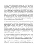
The full-vehicle model of the passenger vehicle considered in this study consists of a single
sprung mass (vehicle body) connected to four unsprung masses and is represented as a 14-
DOF system as shown in Figure 1. The sprung mass is represented as a plane and is allowed
to pitch, roll and yaw as well as to displace in vertical, lateral and longitudinal directions.
The unsprung masses are allowed to bounce vertically with respect to the sprung mass.
Each wheel is also allowed to rotate along its axis and only the two front wheels are free to
steer.
2.1 Modeling Assumptions
Some of the modeling assumptions considered in this study are as follows: the vehicle body
is lumped into a single mass which is referred to as the sprung mass, aerodynamic drag
force is ignored, and the roll centre is coincident with the pitch centre and located just below
the body center of gravity. The suspensions between the sprung mass and unsprung masses
are modeled as passive viscous dampers and spring elements. Rolling resistance due to
passive stabilizer bar and body flexibility are neglected. The vehicle remains grounded at all
times and the four tires never lost contact with the ground during maneuvering. A 4 degrees
tilt angle of the suspension system toward vertical axis is neglected (
4cos
= 0.998
1). Tire
vertical behavior is represented as a linear spring without damping, while the lateral and
longitudinal behaviors are represented with Calspan model. Steering system is modeled as a
constant ratio and the effect of steering inertia is neglected.
2.2 Vehicle Ride Model
The vehicle ride model is represented as a 7-DOF system. It consists of a single sprung mass
(car body) connected to four unsprung masses (front-left, front-right, rear-left and rear-right
wheels) at each corner of the vehicle body. The sprung mass is free to heave, pitch and roll
while the unsprung masses are free to bounce vertically with respect to the sprung mass.
The suspensions between the sprung mass and unsprung masses are modeled as passive
viscous dampers and spring elements. While, the tires are modeled as simple linear springs
without damping. For simplicity, all pitch and roll angles are assumed to be small. A similar
model was used by Ikenaga (2000).
Fig. 1. A 14-DOF full vehicle ride and handling model
Referring to Figure 1, the force balance on sprung mass is given as
ssprrprlpfrpflrrrlfrfl
ZmFFFFFFFF
(1)
where,
F
fl
= suspension force at front left corner
F
fr
= suspension force at front right corner
F
rl
= suspension force at rear left corner
F
rr
= suspension force at rear right corner
m
s
= sprung mass weight
s
Z
= sprung mass acceleration at body centre of gravity
prrprlpfrpfl
FFFF ;;;
= pneumatic actuator forces at front left, front right, rear left and
rear right corners, respectively.
need less fine tuning works. For the purpose of vehicle model validation, an instrumented
experimental vehicle has been developed using a Malaysia National Car. Two types of road
test namely step steer and double lane change test were performed using the instrumented
experimental vehicle. The data obtained from the road tests are used as the validation
benchmarks of the 14-DOF full vehicle model.
This chapter is organized as follows: The first section contains introduction and the review
of some related works, followed by mathematical derivations of the 14-DOF full vehicle
model with Calspan tyre model in the second section. The third section introduces the
proposed controller structure for the ARC system. The fourth section presents the results of
validation of the full vehicle model. Furthermore, improvements of vehicle dynamics
performance on simulation studies and experimental tests using the proposed ARC system
are presented in the fifth and the sixth section, respectively. The last section contains some
conclusions.
2. Full Vehicle Modeling with Calspan Tire Model
The full-vehicle model of the passenger vehicle considered in this study consists of a single
sprung mass (vehicle body) connected to four unsprung masses and is represented as a 14-
DOF system as shown in Figure 1. The sprung mass is represented as a plane and is allowed
to pitch, roll and yaw as well as to displace in vertical, lateral and longitudinal directions.
The unsprung masses are allowed to bounce vertically with respect to the sprung mass.
Each wheel is also allowed to rotate along its axis and only the two front wheels are free to
steer.
2.1 Modeling Assumptions
Some of the modeling assumptions considered in this study are as follows: the vehicle body
is lumped into a single mass which is referred to as the sprung mass, aerodynamic drag
force is ignored, and the roll centre is coincident with the pitch centre and located just below
the body center of gravity. The suspensions between the sprung mass and unsprung masses
are modeled as passive viscous dampers and spring elements. Rolling resistance due to
passive stabilizer bar and body flexibility are neglected. The vehicle remains grounded at all
times and the four tires never lost contact with the ground during maneuvering. A 4 degrees
tilt angle of the suspension system toward vertical axis is neglected (
4cos
= 0.998
1). Tire
vertical behavior is represented as a linear spring without damping, while the lateral and
longitudinal behaviors are represented with Calspan model. Steering system is modeled as a
constant ratio and the effect of steering inertia is neglected.
2.2 Vehicle Ride Model
The vehicle ride model is represented as a 7-DOF system. It consists of a single sprung mass
(car body) connected to four unsprung masses (front-left, front-right, rear-left and rear-right
wheels) at each corner of the vehicle body. The sprung mass is free to heave, pitch and roll
while the unsprung masses are free to bounce vertically with respect to the sprung mass.
The suspensions between the sprung mass and unsprung masses are modeled as passive
viscous dampers and spring elements. While, the tires are modeled as simple linear springs
without damping. For simplicity, all pitch and roll angles are assumed to be small. A similar
model was used by Ikenaga (2000).
Fig. 1. A 14-DOF full vehicle ride and handling model
Referring to Figure 1, the force balance on sprung mass is given as
ssprrprlpfrpflrrrlfrfl
ZmFFFFFFFF
(1)
where,
F
fl
= suspension force at front left corner
F
fr
= suspension force at front right corner
F
rl
= suspension force at rear left corner
F
rr
= suspension force at rear right corner
m
s
= sprung mass weight
s
Z
= sprung mass acceleration at body centre of gravity
prrprlpfrpfl
FFFF ;;;
= pneumatic actuator forces at front left, front right, rear left and
rear right corners, respectively.
PID Control, Implementation and Tuning56
The suspension force at each corner of the vehicle is defined as the sum of the forces
produced by suspension components namely spring force and damper force as the
followings
rrsrrurrsrrsrrurrsrr
rlsrlurlsrlsrlurlsrl
frsfrufrsfrsfrufrsfr
flsfluflsflsfluflsfl
ZZCZZKF
ZZCZZKF
ZZCZZKF
ZZCZZKF
,,,,,,
,,,,,,
,,,,,,
,,,,,,
(2)
where,
K
s,fl
= front left suspension spring stiffness
K
s,fr
= front right suspension spring stiffness
K
s,rr
= rear right suspension spring stiffness
K
s,rl
= rear left suspension spring stiffness
C
s,fr
= front right suspension damping
C
s,fl
= front left suspension damping
C
s,rr
= rear right suspension damping
C
s,rl
= rear left suspension damping
fru
Z
,
= front right unsprung mass displacement
flu
Z
,
= front left unsprung mass displacement
rru
Z
,
= rear right unsprung mass displacement
rlu
Z
,
= rear left unsprung mass displacement
fru
Z
,
= front right unsprung mass velocity
flu
Z
,
= front left unsprung mass velocity
rru
Z
,
= rear right unsprung mass velocity
rlu
Z
,
= rear left unsprung mass velocity
The sprung mass position at each corner can be expressed in terms of bounce, pitch and roll
given by
sin5.0sin
sin5.0sin
sin5.0sin
sin5.0sin
,
,
,
,
wlZZ
wlZZ
wlZZ
wlZZ
rsrrs
rsrls
fsfrs
fsfls
(3)
It is assumed that all angles are small, therefore Eq. (3) becomes
wlZZ
wlZZ
wlZZ
wlZZ
rsrrs
rsrls
fsfrs
fsfls
5.0
5.0
5.0
5.0
,
,
,
,
(4)
where,
l
f
= distance between front of vehicle and center of gravity of sprung mass
l
r
= distance between rear of vehicle and center of gravity of sprung mass
w = track width
= pitch angle at body centre of gravity
= roll angle at body centre of gravity
fls
Z
,
= front left sprung mass displacement
frs
Z
,
= front right sprung mass displacement
rls
Z
,
= rear left sprung mass displacement
rrs
Z
,
= rear right sprung mass displacement
By substituting Eq. (4) and its derivative (sprung mass velocity at each corner) into Eq. (2)
and the resulting equations are then substituted into Eq. (1), the following equation is
obtained
θ
rs
C
r
l
fs
K
f
l
s
Z
rs
C
fs
C
s
Z
rs
K
fs
K
s
Z
s
m
,,
2
,,
2
,,
2
fru
Z
sf
K
flu
Z
fs
C
flu
Z
sf
Kθ
rs
C
r
l
fs
C
f
l
,,,,,,
2
(5)
rru
Z
rs
C
rru
Z
sr
K
rlu
Z
rs
C
rlu
Z
sr
K
fru
Z
fs
C
,,,,,,,,
+
prr
F
prl
F
pfr
F
pfl
F
where,
= pitch rate at body centre of gravity
s
Z
= sprung mass displacement at body centre of gravity
s
Z
= sprung mass velocity at body centre of gravity
K
s,f
= spring stiffness of front suspension (K
s,fl
= K
s,fr
)
K
s,r
= spring stiffness of rear suspension (K
s,rl
= K
s,rr
)
C
s,f
= C
s,fl
= C
s,fr
= damping constant of front suspension
C
s,r
= C
s,rl
= C
s,rr
= damping constant of rear suspension
PID Control, Implementation and Tuning58
Similarly, moment balance equations are derived for pitch
and roll
, and are given as
θKlKlZClClZKlKlθI
rsrfsfsrsr
fs
fsrsr
fs
fyy ,
2
,
2
,
,
,
,
222
fru
fs
fflufsfflu
fs
frsrfsf
ZKlZClZKlθClCl
,
,
,,,
,
,
2
,
2
2
(6)
rr,ur,srrr,ur,srrl,ur,srrl,ur,srfr,uf,sf
ZClZKlZClZKlZCl
rprrprlfpfrpfl
lFFlFF )()(
flufsrsfsrsfsxx
ZwKCCwKKwI
,,,,
2
,,
2
5.05.05.0
frufsfrufsflufs
ZwCZwKZwC
,,,,,,
5.05.05.0
(7)
rrursrrursrlursrlurs
ZwCZwKZwCZwK
,,,,,,,,
5.05.05.05.0
2
)(
2
)(
w
FF
w
FF
prrpfrprlpfl
where,
= pitch acceleration at body centre of gravity
= roll acceleration at body centre of gravity
I
xx
= roll axis moment of inertia
I
yy
= pitch axis moment of inertia
By performing force balance analysis at the four wheels, the following equations are
obtained
fsfsffsfsfssfsfluu
wKClKlZCZKZm
,,,,,,
5.0
pflflrtflufsflutfsfs
FZKZCZKKwC
,,,,,,
5.0
(8)
fsfsffsfsfssfsfruu
wKClKlZCZKZm
,,,,,,
5.0
pfrfrrtfrufsfrutfsfs
FZKZCZKKwC
,,,,,,
5.0
(9)
rsrsrrsrsrssrsrluu
wKClKlZCZKZm
,,,,,,
5.0
prlrlrtrlursrlutrsrs
FZKZCZKKwC
,,,,,.
5.0
(10)
rsrsrrsrsrssrsrruu
wKClKlZCZKZm
,,,,,,
5.0
prrrrrtrrursrrutrsrs
FZKZCZKKwC
,,,,,,
5.0
(11)
where,
fru
Z
,
= front right unsprung mass acceleration
flu
Z
,
= front left unsprung mass acceleration
rru
Z
,
= rear right unsprung mass acceleration
rlu
Z
,
= rear left unsprung mass acceleration
rlrrrrflrfrr
ZZZZ
,,,,
= road profiles at front left, front right, rear right
and rear left tyres respectively
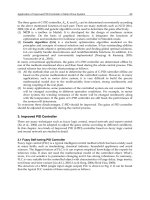
2.3 Vehicle Handling Model
The handling model employed in this paper is a 7-DOF system as shown in Figure 2. It takes
into account three degrees of freedom for the vehicle body in lateral and longitudinal
motions as well as yaw motion (r) and one degree of freedom due to the rotational motion of
each tire. In vehicle handling model, it is assumed that the vehicle is moving on a flat road.
The vehicle experiences motion along the longitudinal x-axis and the lateral y-axis, and the
angular motions of yaw around the vertical z-axis. The motion in the horizontal plane can be
characterized by the longitudinal and lateral accelerations, denoted by a
x
and a
y
respectively,
and the velocities in longitudinal and lateral direction, denoted by
x
v
and
y
v
, respectively.
Fig. 2. A 7-DOF vehicle handling model
Similarly, moment balance equations are derived for pitch
and roll
, and are given as
θKlKlZClClZKlKlθI
rsrfsfsrsr
fs
fsrsr
fs
fyy ,
2
,
2
,
,
,
,
222
fru
fs
fflufsfflu
fs
frsrfsf
ZKlZClZKlθClCl
,
,
,,,
,
,
2
,
2
2
(6)
rr,ur,srrr,ur,srrl,ur,srrl,ur,srfr,uf,sf
ZClZKlZClZKlZCl
rprrprlfpfrpfl
lFFlFF )()(
flufsrsfsrsfsxx
ZwKCCwKKwI
,,,,
2
,,
2
5.05.05.0
frufsfrufsflufs
ZwCZwKZwC
,,,,,,
5.05.05.0
(7)
rrursrrursrlursrlurs
ZwCZwKZwCZwK
,,,,,,,,
5.05.05.05.0
2
)(
2
)(
w
FF
w
FF
prrpfrprlpfl
where,
= pitch acceleration at body centre of gravity
= roll acceleration at body centre of gravity
I
xx
= roll axis moment of inertia
I
yy
= pitch axis moment of inertia
By performing force balance analysis at the four wheels, the following equations are
obtained
fsfsffsfsfssfsfluu
wKClKlZCZKZm
,,,,,,
5.0
pflflrtflufsflutfsfs
FZKZCZKKwC
,,,,,,
5.0
(8)
fsfsffsfsfssfsfruu
wKClKlZCZKZm
,,,,,,
5.0
pfrfrrtfrufsfrutfsfs
FZKZCZKKwC
,,,,,,
5.0
(9)
rsrsrrsrsrssrsrluu
wKClKlZCZKZm
,,,,,,
5.0
prlrlrtrlursrlutrsrs
FZKZCZKKwC
,,,,,.
5.0
(10)
rsrsrrsrsrssrsrruu
wKClKlZCZKZm
,,,,,,
5.0
prrrrrtrrursrrutrsrs
FZKZCZKKwC
,,,,,,
5.0
(11)
where,
fru
Z
,
= front right unsprung mass acceleration
flu
Z
,
= front left unsprung mass acceleration
rru
Z
,
= rear right unsprung mass acceleration
rlu
Z
,
= rear left unsprung mass acceleration
rlrrrrflrfrr
ZZZZ
,,,,
= road profiles at front left, front right, rear right
and rear left tyres respectively
2.3 Vehicle Handling Model
The handling model employed in this paper is a 7-DOF system as shown in Figure 2. It takes
into account three degrees of freedom for the vehicle body in lateral and longitudinal
motions as well as yaw motion (r) and one degree of freedom due to the rotational motion of
each tire. In vehicle handling model, it is assumed that the vehicle is moving on a flat road.
The vehicle experiences motion along the longitudinal x-axis and the lateral y-axis, and the
angular motions of yaw around the vertical z-axis. The motion in the horizontal plane can be
characterized by the longitudinal and lateral accelerations, denoted by a
x
and a
y
respectively,
and the velocities in longitudinal and lateral direction, denoted by
x
v
and
y
v
, respectively.
Fig. 2. A 7-DOF vehicle handling model
PID Control, Implementation and Tuning60
Acceleration in longitudinal x-axis is defined as
rvav
yx
x
(12)
By summing all the forces in x-axis, longitudinal acceleration can be defined as
t
xrrxrlyfrxfryflxfl
x
m
FFFFFF
a
sincossincos
(13)
Similarly, acceleration in lateral y-axis is defined as
rvav
xy
y
(14)
By summing all the forces in lateral direction, lateral acceleration can be defined as
t
yrryrlxfryfrxflyfl
y
m
FFFFFF
a
sincossincos
(15)
where
xij
F
and
yij
F
denote the tire forces in the longitudinal and lateral directions,
respectively, with the index (i) indicating front (f) or rear (r) tires and index (j) indicating left
(l) or right (r) tires. The steering angle is denoted by δ, the yaw rate by
.
r
and
t
m
denotes the
total vehicle mass. The longitudinal and lateral vehicle velocities
x
v
and
y
v
can be obtained
by integrating of
y
v
.
and
x
v
.
. They can be used to obtain the side slip angle, denoted by α.
Thus, the slip angle of front and rear tires are found as
f
x
fy
f
δ
v
rlv
α
1
tan
; (16)
and
x
ry
r
v
rlv
α
1
tan
(17)
where,
f
and
r
are the side slip angles at front and rear tires respectively. While l
f
and l
r
are the distance between front and rear tire to the body center of gravity respectively.
To calculate the longitudinal slip, longitudinal component of the tire velocity should be
derived. The front and rear longitudinal velocity component is given by:
ftfwxf
Vv
cos
(18)
where, the speed of the front tire is,
2
2
xfytf
vrlvV
(19)
The rear longitudinal velocity component is,
rtrwxr
Vv
cos
(20)
where, the speed of the rear tire is,
2
2
xrytr
vrlvV
(21)
Then, the longitudinal slip ratio of front tire,
wxf
wfwxf
af
v
Rv
S
, under braking conditions (22)
The longitudinal slip ratio of rear tire is,
wxr
wrwxr
ar
v
Rv
S
, under braking conditions (23)
where, ω
r
and ω
f
are angular velocities of rear and front tires, respectively and
w
R , is the
wheel radius.
The yaw motion is also dependent on the tire forces
xij
F
and
yij
F
as well as
on the self-aligning moments, denoted by
zij
M
acting on each tire:
zrrzrlzfrzflxfrf
xflfyfrfyflfyrrryrlryfr
yflxrrxrlxfrxfl
z
MMMMFl
FlFlFlFlFlF
w
F
w
F
w
F
w
F
w
F
w
J
r
sin
sincoscossin
2
sin
222
cos
2
cos
2
1
(24)
PID Control, Implementation and Tuning62
where,
z
J
is the moment of inertia around the z-axis. The roll and pitch motion depend very
much on the longitudinal and lateral accelerations. Since only the vehicle body undergoes
roll and pitch, the sprung mass, denoted by
s
m
has to be considered in determining the
effects of handling on pitch and roll motions as the following:
sx
sys
J
kgcmcam
.
(25)
sy
sys
J
kgcmcam
.
(26)
where, c is the height of the sprung mass center of gravity from the ground,
g
is the
gravitational acceleration and
k
,
,
k and
are the damping and stiffness constant for
roll and pitch, respectively. The moments of inertia of the sprung mass around x-axis and y-
axis are denoted by
sx
J and
sy
J
respectively.
2.4 Simplified Calspan Tire Model
Tire model considered in this study is Calspan model as described in Szostak et al. (1988).
Calspan model is able to describe the behavior of a vehicle in any driving scenario including
inclement driving conditions which may require severe steering, braking, acceleration, and
other driving related operations (Kadir et al., 2008). The longitudinal and lateral forces
generated by a tire are a function of the slip angle and longitudinal slip of the tire relative to
the road. The previous theoretical developments in Szostak et al. (1988) lead to a complex,
highly non-linear composite force as a function of composite slip. It is convenient to define a
saturation function, f(σ), to obtain a composite force with any normal load and coefficient of
friction values (Singh et al., 2000). The polynomial expression of the saturation function is
presented by:
1
)
4
(
)(
4
2
2
3
1
2
2
3
1
CCC
CC
F
F
f
z
c
(27)
where, C
1
, C
2
, C
3
and C
4
are constant parameters fixed to the specific tires. The tire contact
patch lengths are calculated using the following two equations:
5
0768.0
0
pw
ZTz
TT
FF
ap
(28)
z
xa
F
FK
ap 1
(29)
where
ap
is the tire contact patch, F
z
is a normal force, T
w
is a tread width, and T
p
is a tire
pressure. While F
ZT
and K
α
are tire contact patch constants. The lateral and longitudinal
stiffness coefficients (K
s
and K
c
, respectively) are a function of tire contact patch length and
normal load of the tire as expressed as follows:
2
2
1
10
2
0
2
A
FA
FAA
ap
K
z
zs
(30)
FZCSF
ap
K
zc
/
2
2
0
(31)
where the values of A
0
, A
1
, A
2
and CS/FZ are stiffness constants. Then, the composite slip
calculation becomes:
2
2
2
2
0
2
1
tan
8
s
s
KK
F
ap
cs
z
(32)
Where S is a tire longitudinal slip,
is a tire slip angle, and µ
o
is a nominal coefficient of
friction and has a value of 0.85 for normal road conditions, 0.3 for wet road conditions, and
0.1 for icy road conditions. Given the polynomial saturation function, lateral and
longitudinal stiffness, the normalized lateral and longitudinal forces are derived by
resolving the composite force into the side slip angle and longitudinal slip ratio components:
Y
SKK
Kf
F
F
cs
s
z
y
2
2
'2
2
tan
tan
(33)
2
2
'2
2
'
tan SKK
SKf
F
F
cs
c
z
x
(34)
Lateral force has an additional component due to the tire camber angle, γ, which is modeled
as a linear effect. Under significant maneuvering conditions with large lateral and
longitudinal slip, the force converges to a common sliding friction value. In order to meet
PID Control, Implementation and Tuning64
this criterion, the longitudinal stiffness coefficient is modified at high slips to transition to
lateral stiffness coefficient as well as the coefficient of friction defined by the parameter K
µ
.
222'
cossin SKKKK
cscc
(35)
222
0
cossin1 SK
(36)
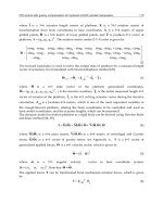
3. Controller Structure of Pneumatically Actuated
Active Roll Control Suspension System
The proposed controller structure consists of inner loop controller to reject the unwanted
weight transfer and outer loop controller to stabilize heave and roll responses due to
steering wheel input from the driver. An input decoupling transformation is placed between
inner and outer loop controllers that blend the inner loop and outer loop controller. The
outer loop controller provides the ride control that isolates the vehicle body from vertical
and rotational vibrations induced by steering wheel input and the inner loop controller
provides the weight transfer rejection control that maintains load-leveling and load
distribution during vehicle maneuvers. The proposed control structure is shown in Figure 3.
Fig. 3. The proposed control structure for arc system
The outputs of the outer loop controller are vertical forces to stabilize body bounce
z
M
and moment to stabilize roll
M
. These forces and moments are then distributed into
target forces of the four pneumatic actuators produced by the outer loop controller.
Distribution of the forces and moments into target forces of the four pneumatic actuators is
performed using decoupling transformation subsystem. The outputs of the decoupling
transformation subsystem namely the target forces of the four pneumatic actuators are then
subtracted with the relevant outputs from the inner loop controller to produce the ideal
target forces of the four pneumatic actuators. Decoupling transformation subsystem
requires an understanding of the system dynamics in the previous section. The equivalent
force and moment for heave, pitch and roll can be defined by
"
prr
"
prl
"
pfr
"
pflz
FFFFF
(37)
r
"
prrr
"
prlf
"
pfrf
"
pfl
lFlFlFlFM
(38)
2222
w
F
w
F
w
F
w
FM
"
prr
"
prl
"
pfr
"
pfl
(39)
where
""""
,,
prrprlpfrpfl
FFFF
are the pneumatic forces produced by outer loop controller
in front left, front right, rear left and rear right corners, respectively. In the case of the
vehicle input comes from steering wheel, the pitch moment can be neglected. Equations (37),
(38) and (39) can be rearranged in matrix format as the following
"
"
"
"
2222
1111
)(
prr
prl
pfr
pfl
rrff
z
F
F
F
F
wwww
llll
tM
tM
tF
(40)
For a linear system of equations y=Cx, if C
mxn
has full row rank, then there exists a
right inverse C
-1
such that C-1 C= 1
mxm
. The right inverse can be computed using C
-
1
=C
T
(CC
T
)
-1
. Thus, the inverse relationship of equation (40) can be expressed as:
M
M
F
w)ll()ll(
l
w)ll()ll(
l
w)ll()ll(
l
w)ll()ll(
l
F
F
F
F
z
rfrf
f
rfrf
f
rfrf
r
rfrf
r
"
prr
"
prl
"
pfr
"
pfl
2
1
2
1
2
2
1
2
1
2
2
1
2
1
2
2
1
2
1
2
(41)
In the outer loop controller, PID control is applied for suppressing both body vertical
displacement and body roll angle. The inner loop controller of roll moment rejection control
is described as follows: during cornering, a vehicle will produce a sideway force namely
cornering force at the body center of gravity. The cornering force generates roll moment to
this criterion, the longitudinal stiffness coefficient is modified at high slips to transition to
lateral stiffness coefficient as well as the coefficient of friction defined by the parameter K
µ
.
222'
cossin SKKKK
cscc
(35)
222
0
cossin1 SK
(36)
3. Controller Structure of Pneumatically Actuated
Active Roll Control Suspension System
The proposed controller structure consists of inner loop controller to reject the unwanted
weight transfer and outer loop controller to stabilize heave and roll responses due to
steering wheel input from the driver. An input decoupling transformation is placed between
inner and outer loop controllers that blend the inner loop and outer loop controller. The
outer loop controller provides the ride control that isolates the vehicle body from vertical
and rotational vibrations induced by steering wheel input and the inner loop controller
provides the weight transfer rejection control that maintains load-leveling and load
distribution during vehicle maneuvers. The proposed control structure is shown in Figure 3.
Fig. 3. The proposed control structure for arc system
The outputs of the outer loop controller are vertical forces to stabilize body bounce
z
M
and moment to stabilize roll
M
. These forces and moments are then distributed into
target forces of the four pneumatic actuators produced by the outer loop controller.
Distribution of the forces and moments into target forces of the four pneumatic actuators is
performed using decoupling transformation subsystem. The outputs of the decoupling
transformation subsystem namely the target forces of the four pneumatic actuators are then
subtracted with the relevant outputs from the inner loop controller to produce the ideal
target forces of the four pneumatic actuators. Decoupling transformation subsystem
requires an understanding of the system dynamics in the previous section. The equivalent
force and moment for heave, pitch and roll can be defined by
"
prr
"
prl
"
pfr
"
pflz
FFFFF
(37)
r
"
prrr
"
prlf
"
pfrf
"
pfl
lFlFlFlFM
(38)
2222
w
F
w
F
w
F
w
FM
"
prr
"
prl
"
pfr
"
pfl
(39)
where
""""
,,
prrprlpfrpfl
FFFF
are the pneumatic forces produced by outer loop controller
in front left, front right, rear left and rear right corners, respectively. In the case of the
vehicle input comes from steering wheel, the pitch moment can be neglected. Equations (37),
(38) and (39) can be rearranged in matrix format as the following
"
"
"
"
2222
1111
)(
prr
prl
pfr
pfl
rrff
z
F
F
F
F
wwww
llll
tM
tM
tF
(40)
For a linear system of equations y=Cx, if C
mxn
has full row rank, then there exists a
right inverse C
-1
such that C-1 C= 1
mxm
. The right inverse can be computed using C
-
1
=C
T
(CC
T
)
-1
. Thus, the inverse relationship of equation (40) can be expressed as:
M
M
F
w)ll()ll(
l
w)ll()ll(
l
w)ll()ll(
l
w)ll()ll(
l
F
F
F
F
z
rfrf
f
rfrf
f
rfrf
r
rfrf
r
"
prr
"
prl
"
pfr
"
pfl
2
1
2
1
2
2
1
2
1
2
2
1
2
1
2
2
1
2
1
2
(41)
In the outer loop controller, PID control is applied for suppressing both body vertical
displacement and body roll angle. The inner loop controller of roll moment rejection control
is described as follows: during cornering, a vehicle will produce a sideway force namely
cornering force at the body center of gravity. The cornering force generates roll moment to
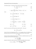
PID Control, Implementation and Tuning66
the roll center causing the body center of gravity to shift outward as shown in Figure 4.
Shifting the body center of gravity causes a weight transfer from the inside toward the
outside wheels. By defining b as the distance between body center of gravity and the roll
center, roll moment is defined by
baMM
ysr
(42)
The two pneumatic actuators installed in outside wheels have to produce the necessary
forces to cancel out the unwanted roll moments, whereas the forces of the two pneumatic
actuators in inside wheels are set to zero. Pneumatic force to cancel out roll moment in each
corner for counter clockwise steering wheel input is defined as:
2
/
''
w
baM
FF
ys
prrpfr
and
0
''
prlpfl
FF
(43)
Whereas, pneumatic force to cancel out roll moment in each corner for clockwise steering
wheel input can be defined as:
2/
''
w
baM
FF
ys
pflprl
and
0
''
prrpfr
FF
(44)
where,
'
pfl
F
= target force of pneumatic system at front left corner produced by inner loop controller
'
pfr
F
= target force of pneumatic system at front right corner produced by inner loop
controller
'
prl
F
= target force of pneumatic system at rear left corner produced by inner loop controller
'
prr
F
= target force of pneumatic system at rear right corner produced by inner loop
controller
The ideal target forces for each pneumatic actuator are defined as the target forces produced
by outer loop controller subtracted with the respective target forces produced by inner loop
controller as the following:
'
pfl
"
pflpfl
FFF
(45)
'
pfr
"
pfrpfr
FFF
(46)
'
prl
"
prlprl
FFF
(47)
'
prr
"
prrprr
FFF
(48)
Fig. 4. Roll Moment Generated by Lateral Force
4. Validation of 14-DOF Ride and Handling Model
To verify the full vehicle ride and handling model, experimental works were performed
using an instrumented experimental vehicle. This section provides the verification of ride
and handling model using visual technique by simply comparing the trend of simulation
results with experimental data using the same input conditions. Validation or verification is
defined as the comparison of model’s performance with a real system. Therefore, the
validation is not meant as fitting the simulated data exactly to the measured data, but as
gaining confidence that the vehicle handling simulation is giving insight into the behavior of
the simulated vehicle. The test data are also used to check whether the input parameters for
the vehicle model are reasonable. In general, model validation can be defined as
determining the acceptability of a model using some statistical tests for deviance measures
or subjectively using visual techniques.
4.1 Instrumented Experimental Vehicle
The data acquisition system (DAS) is installed into the experimental vehicle to obtain the
experimental data from the real vehicle reaction to evaluate the vehicle performance in
terms of lateral acceleration, body vertical acceleration, yaw rate and roll rate. The DAS uses
several types of transducers such as single axis accelerometer to measure the sprung mass
and unsprung mass accelerations for each corner, tri-axial accelerometer to measure lateral,
vertical and longitudinal accelerations at the body center of gravity, steering wheel sensor
and tri-axial gyroscopes for the yaw rate, pitch rate and roll rate. The multi-channel µ-
MUSYCS system Integrated Measurement and Control (IMC) is used as the DAS system.
Online FAMOS software as the real time data processing and display function is used to
ease the data collection. The installation of the DAS and sensors to the experimental vehicle
can be seen in Figure 5.
PID Control, Implementation and Tuning68
Fig. 5. Instrumented experimental vehicle
4.2 Validation Procedures
The dynamic response characteristics of a vehicle model that include yaw response, lateral
acceleration, slip angle in each tire and roll rate can be validated using experimental test
through several handling test procedures namely step steer test and double lane change
(DLC) test. Step steer test is intended to study transient response of the vehicle under
steering wheel input. In this study, step steer tests were performedwith 180 degrees clock
wise at 50 km/h. On the other hand, double-lane change test is used to evaluate road
holding of the vehicle during crash avoidance. In this study, the speed of 80 km/h was set
for the double-lane change test.
4.3 Model Validation Results
In experimental works, all the experimental data were filtered using 5
th
order Butterworth
low pass filter with the cut-off frequency of 5 Hz. It is necessary to note that the measured
steering angle from the steering wheel sensorwas used as the input of simulation model. For
the simulation model, tire parameters are obtained from Szostak et al. (1988) and Singh et al.
(2000). The results of model verification for 180 degrees step steer test at 50 km/h is shown
in Figure 6 to 13.
Figure 6 shows the steering wheel input applied for the step steer test. It can be seen that the
trends between simulation results and experimental data are almost similar with acceptable
error. The small difference in magnitude between simulation and experimental results is
due to the simplification in vehicle dynamics modeling where the effects of anti roll bar
were completely ignored. In fact, the anti roll bar plays an important role in reducing the
vertical and roll responses of vehicle body. In simulation model, vehicle body is assumed to
be rigid. It can be another source of deviation since the body flexibility can influence the roll
effects of the vehicle body.
In terms of yaw rate, lateral acceleration and body roll angle, it can be seen that there are
quite good comparisons during the initial transient phase as well as during the subsequent
steady state phase as shown in Figures 7 to 9. Slip angle responses of the front tires also
show satisfying comparison with only small deviation in the transition area between
transient and steady state phases as shown in Figures 10 and 11.
It can also be noted that the slip angle responses of all tires in the experimental data are
slightly higher than the slip angle data obtained from the simulation particularly for the rear
tires as can be seen in Figures 12 and 13. This is due to the fact that it is difficult for the
driver to maintain a constant speed during maneuvering. In simulation, it is also assumed
that the vehicle is moving on a flat road during step steer maneuver. In fact, it is observed
that the road profiles of test field consist of irregular surface. This can be another source of
deviation on slip angle response of the tires.
Fig. 6. Steer angle input for 180 deg step steer at 50 km/h
Fig. 7. Yaw rate response for 180 deg step steer at 50 km/h
PID Control, Implementation and Tuning70
Fig. 8. Lateral acceleration response for 180 deg step steer at 50 km/h
Fig. 9. Roll angle response for 180 deg step steer at 50 km/h
Fig. 10. Slip angle at the front left tire for 180 deg step steer at 50 km/h
Fig. 11. Slip angle response at front right tire for 180 deg step steer at 50 km/h
Fig. 12. Slip angle at the rear right tire for 180 deg step steer at 50 km/h
Fig. 13. Slip angle at the rear left tire for 180 deg step steer at 50 km/h
The results of double lane change test indicate that measurement data and the simulation
results agree with a relatively good accuracy as shown in Figures 14 to 21. Figure 14 shows
PID Control, Implementation and Tuning72
the measured steering wheel input from double lane change test maneuver which is also
used as the input for the simulation model. In terms of yaw rate, lateral acceleration and
body roll angle, it is clear that the simulation results closely follow the measured data with
minor difference in magnitude as shown in Figures 15 to 17. The minor difference in
magnitude and small fluctuation occurred on the measured data is due to the body
flexibility which was ignored in the simulation model. The minor difference in magnitude
between measured and simulated data can also be caused by one of the modeling
assumptions namely the effects of anti roll bar which is completely ignored in simulation
model.
In terms of tire side slip angles, the trends of simulation results have a good correlation with
experimental data as can be seen in Figures 18 to 21. Almost similar to the validation results
obtained from step steer test, the slip angle responses of all tires in experimental data are
higher than the slip angle data obtained from the simulation particularly for the rear tires.
Again, this is due to the difficulty of the driver to maintain a constant speed during double
lane change maneuver. Assumption in simulation model that the vehicle is moving on a flat
road during double lane change maneuver is also very difficult to realize in practice. In fact,
road irregularities of the test field may cause the change in tire properties during vehicle
handling test. Assumption of neglecting the steering inertia have the possibility in lowering
down the magnitude of tire side slip angle in simulation results compared to the measured
data.
Overall, it can be concluded that the trends between simulation results and experimental
data are having good agreement with acceptable error. The error could be significantly
reduced by fine tuning of both vehicle and tire parameters. However, excessive fine tuning
works can be avoided since in control oriented model, the most important characteristic is
the trend of the model response. As long as the trend of the model response is closely
similar with the measured response with acceptable deviation in magnitude, it can be said
that the model is valid. The validated model will be used in conjunction with the proposed
controller structure of the ARC system in the next section.
Fig. 14. Steer angle input for 80 km/h double lane change maneuver
Fig. 15. Yaw rate response for 80 km/h double lane change maneuver
Fig. 16. Lateral acceleration response for 80 km/h double lane change maneuver
Fig. 17. Roll angle response for 80 km/h double lane change maneuver