PID Control Implementation and Tuning Part 7 pptx

PID control with gravity compensation for hydraulic 6-DOF parallel manipulator 113


Fig. 1. Configuration of 6-DOF Gough-Stewart platform


Fig. 2. Definition of the Cartesian coordination systems and vectors in dynamics and
kinematics equations of

6-DOF Gough-Stewart platform

For the movement including the linear and angular motions of Gough-Stewart platform, the
inverse kinematics model is derived using closed-form solution [22].


cBARl
~
)
~
~
(
~
 (1)

where l
~
is a 3×6 actuator length matrix of platform, R is a 3×3 rotation matrix of
transformation from body coordinates to base coordinates,
A
~
is a 3×6 matrix of upper

gimbal points,
B
~
is a 3×6 matrix of lower gimbal points, and c
~
is position 3×1 vector of
platform,
T
321
),,(
~
qqqc . The rotation matrix under Z-Y-X order is given by















45455
464564564656
456464645665

coscossincossin
sincoscossinsinsinsinsincoscoscossin
cossincossinsincossinsinsincoscoscos
qqqqq
qqqqqqqqqqqq
qqqqqqqqqqqq
R

(2)
The forward kinematics is used to solve the output state of platform for a measured length
vector of actuators; it is formulated with Newton-Raphson method [23].


)
~
~
(
~
~
0
1
~
,
1 j
l
jj
llJΘΘ 




(3)

where Θ
~
is a 6×1 state vector of the platform generalized coordinates,
T
654321
),,,,,(
~
qqqqqqΘ , j is the iterative numbers,
0
~
l is the initial measured length 6×1
vector of actuator of the platform,
j
l
~
is the 6×1 solving actuator vector during the iterative
calculation,

~
,l
J is a Jacobian 6×6 matrix, which is one of the most important variables in
the Gough-Stewart platform, relating the body coordinates to be controlled and used as
basic model coordinates, and the actuator lengths, which can be measured.
The dynamic model for motion platform as a rigid body can be derived using Newton-Euler
and Kane method [24, 25].

ΘΘΘVΘΘMΘGτ


 ),
~
(
~
)
~
(
~
)
~
(
~
~
(4)

where )
~
(
~
ΘM is a 6×6 mass matrix, ),
~
(
~
ΘΘV

is a 6×6 matrix of centrifugal and Coriolis
terms,
)
~
(

~
ΘG
is a 6×1 vector of gravity terms, see Appendix A, τ
~
is a 6×1 vector of
generalized applied forces,
Θ

is a 6×1 velocity vector, which is given by


T
)
~
~
( ωcΘ



(5)

where ω
~
is a 3×1 angular velocity vector in base coordinate system,
T
)(
~
zyx

ω .Note that ΘΘ



~
 .
The applied forces
τ can be transformed from mechanism actuator forces, which is given
by

a
T
~
,
~
FJτ 
l
(6)

PID Control, Implementation and Tuning114

where F
a
is a 6×1 vector representing actuator forces,
T
6a2a1aa
)( fff F , f
ai
(i=1,…,6) is actuator output force.
The rotation of actuator around itself is ignored, thus the dynamic model for each hydraulic
actuator (piston rod and cylinder) using Newton-Euler and Kane method is described as

it
T
Θ
~
ai,
,ai
tcu
T
Θ
~
ai,
,ai
uc
)()( FgJJgJJ  mm 7(a)

)
~
()(
))
~
()()(
bb
T
Θ
~
ai,
,ai
tc
tct

T
Θ
~
ai,
,ai
tcaa
T
Θ
~
ai,
,ai
ucucu
T
Θ
~
ai,
,ai
uci
ii
ii
mm
ωIωωIJJ
vJJωIωωIJJvJJF




7(b)

where

,ai
tc
,ai
uc
,JJ are 3×3 Jacobian matrix,
Θ
~
ai,
, J is 3×6 Jacobian matrix, m
u
is the mass of
piston rod of a actuator, m
t
is the mass of cylinder of a actuator,
i
ω is the angular velocity
of actuator relative to relevant lower gimbal point,
uc
v ,
tc
v are the linear velocity of the
mass center of piston rod and cylinder, respectively,
a
I ,
b
I are the inertia of piston rod and
cylinder, respectively, g is acceleration vector of gravity, g=(0 0 g)
T
.
Combining Eqs.(4), (5),(6) and (7), the dynamics model of 6-DOF Gough-Stewart platform as

thirteen rigid body is obtained with Kane method, given by


ΘΘΘVΘΘMΘGτ

),
~
()
~
()
~
(
~
***
 (8)

where, )
~
(
*
ΘM is a mass matrix, ),
~
(
*
ΘΘV

is a matrix of centrifugal and Coriolis terms,
)
~
(

*
ΘG
is a vector of gravity terms, see Appendix B.
The hydraulic systems are studied in depth for symmetrical servovalve and actuator [26], it
is assumed that Coulomb frictions are zero (Coulomb friction F
ci
<<
ic
lB

, not zero,
practically) the hydraulic system mathematical models of symmetric and matched
servovalve and symmetrical actuator are given as


))(sign(
1
LvsvdL iiii
pxpxwCq 


(9)

iiii
p
E
V
pClAq
L
t

LteL
4


 (10)

fiii
ffpA 
aL
(11)

where
i
q
L
is load flow of the i
th
hydraulic actuator, w is area grads,
i
x
v
is position of the i
th

servovalve,

is fluid density,
s
p is supply pressure of servosystem,
Li

p is load pressure
of the i
th
actuator, A is effective acting area of piston,
te
C is the leakage coefficient,
t
V is
actuator cubage,
E
is bulk modulus of fluid,
i
l is the length of the i
th
actuator, C
d
is flow

coefficient, f
fi
is joint space friction force in the i
th
actuator. A number of methods can be
used to model the friction F
f
[21, 27]. A widely method for modeling friction as


scvf
lll FFFF  )()()(


(12)

where F
f
is total friction vector,
T
61
][
fff
ff F , F
v
, F
c
and F
s
are the viscous,
Coulomb and static friction vector, respectively, with elements










0,0
0,

)(
i
iic
ivi
l
llB
lf



i=1,2, …,6 (13)









0,0
0),(sign
)(
,0
i
iiic
ici
l
llf
lf




i=1,2, …,6 (14)










0,0
0,0||),(
0,0||,
)(
,0,ext,0
,0,ext,ext
i
iiisiiis
iiisii
isi
l
llfflsignf
llfff
lf





i=1,2, …,6 (15)

where B
c
is viscous damping coefficient, f
c0,i
is the element of Coulomb friction, f
ext,i
is the
external force element, f
s0,i
is the breakaway force element.

3. Control design
In this section, the inverse dynamic methodology [20] is adopted to derive a proportional
plus derivative controller with dynamic gravity compensation for 6-DOF hydraulic driven
Gough-Stewart platform in the case in which the system parameters are known, the PDGC
control scheme are described in Fig.3.


Fig. 3. Control block diagram for PDGC

The PDGC controller considered the dynamic characteristic of parallel manipulator
embedded the forward kinematics, dynamic gravity terms and inverse of transfer function
from the input position of servovalve to the output force of actuator and Jacobian
matrix
1
T

)(


l
J in inverse of transpose form in inner control loop. It is should be noted that
PID control with gravity compensation for hydraulic 6-DOF parallel manipulator 115

where F
a
is a 6×1 vector representing actuator forces,
T
6a2a1aa
)( fff F , f
ai
(i=1,…,6) is actuator output force.
The rotation of actuator around itself is ignored, thus the dynamic model for each hydraulic
actuator (piston rod and cylinder) using Newton-Euler and Kane method is described as


it
T
Θ
~
ai,
,ai
tcu
T
Θ
~
ai,

,ai
uc
)()( FgJJgJJ  mm 7(a)

)
~
()(
))
~
()()(
bb
T
Θ
~
ai,
,ai
tc
tct
T
Θ
~
ai,
,ai
tcaa
T
Θ
~
ai,
,ai
ucucu

T
Θ
~
ai,
,ai
uci
ii
ii
mm
ωIωωIJJ
vJJωIωωIJJvJJF




7(b)

where
,ai
tc
,ai
uc
,JJ are 3×3 Jacobian matrix,
Θ
~
ai,
, J is 3×6 Jacobian matrix, m
u
is the mass of
piston rod of a actuator, m

t
is the mass of cylinder of a actuator,
i
ω is the angular velocity
of actuator relative to relevant lower gimbal point,
uc
v ,
tc
v are the linear velocity of the
mass center of piston rod and cylinder, respectively,
a
I ,
b
I are the inertia of piston rod and
cylinder, respectively, g is acceleration vector of gravity, g=(0 0 g)
T
.
Combining Eqs.(4), (5),(6) and (7), the dynamics model of 6-DOF Gough-Stewart platform as
thirteen rigid body is obtained with Kane method, given by


ΘΘΘVΘΘMΘGτ

),
~
()
~
()
~
(

~
***
 (8)

where, )
~
(
*
ΘM is a mass matrix, ),
~
(
*
ΘΘV

is a matrix of centrifugal and Coriolis terms,
)
~
(
*
ΘG
is a vector of gravity terms, see Appendix B.
The hydraulic systems are studied in depth for symmetrical servovalve and actuator [26], it
is assumed that Coulomb frictions are zero (Coulomb friction F
ci
<<
ic
lB

, not zero,
practically) the hydraulic system mathematical models of symmetric and matched

servovalve and symmetrical actuator are given as


))(sign(
1
LvsvdL iiii
pxpxwCq 


(9)

iiii
p
E
V
pClAq
L
t
LteL
4


 (10)

fiii
ffpA



aL

(11)

where
i
q
L
is load flow of the i
th
hydraulic actuator, w is area grads,
i
x
v
is position of the i
th

servovalve,

is fluid density,
s
p is supply pressure of servosystem,
Li
p is load pressure
of the i
th
actuator, A is effective acting area of piston,
te
C is the leakage coefficient,
t
V is
actuator cubage,

E
is bulk modulus of fluid,
i
l is the length of the i
th
actuator, C
d
is flow

coefficient, f
fi
is joint space friction force in the i
th
actuator. A number of methods can be
used to model the friction F
f
[21, 27]. A widely method for modeling friction as


scvf
lll FFFF  )()()(

(12)

where F
f
is total friction vector,
T
61
][

fff
ff F , F
v
, F
c
and F
s
are the viscous,
Coulomb and static friction vector, respectively, with elements










0,0
0,
)(
i
iic
ivi
l
llB
lf




i=1,2, …,6 (13)









0,0
0),(sign
)(
,0
i
iiic
ici
l
llf
lf



i=1,2, …,6 (14)











0,0
0,0||),(
0,0||,
)(
,0,ext,0
,0,ext,ext
i
iiisiiis
iiisii
isi
l
llfflsignf
llfff
lf




i=1,2, …,6 (15)

where B
c
is viscous damping coefficient, f
c0,i
is the element of Coulomb friction, f

ext,i
is the
external force element, f
s0,i
is the breakaway force element.

3. Control design
In this section, the inverse dynamic methodology [20] is adopted to derive a proportional
plus derivative controller with dynamic gravity compensation for 6-DOF hydraulic driven
Gough-Stewart platform in the case in which the system parameters are known, the PDGC
control scheme are described in Fig.3.


Fig. 3. Control block diagram for PDGC

The PDGC controller considered the dynamic characteristic of parallel manipulator
embedded the forward kinematics, dynamic gravity terms and inverse of transfer function
from the input position of servovalve to the output force of actuator and Jacobian
matrix
1
T
)(


l
J in inverse of transpose form in inner control loop. It is should be noted that
PID Control, Implementation and Tuning116

the friction force, zero bias and dead zone of servovalve also affect the steady and dynamic
precision as well as system gravity. However, the valve with high performance index may

be chosen to avoid the effect of dead zone of control valve. In fact, the dead zone of
servovalve in hydraulic system is very small, which can achieve 0.01mm even a general
servovalve. The zero bias of servovalve may be measured and compensated for control
system. For large hydraulic parallel manipulator with heavy payload, the system gravity is
much more that the maximal friction even that no payload exist in hydraulic 6-DOF parallel
manipulator. Therefore, the dynamical gravity, the most chief influencing factor of steady
precision, and viscous friction is taken into account for designing of the developed control
scheme without considering Column and static friction in this paper. Besides, the classical
PID is widely applied in hydraulic 6-DOF parallel manipulator in practice, then the
considered system gravity is associated with PID control to improve the steady and
dynamic precision without destroy the steadily of the original control system.
The nature frequency of servovalve is higher than the mechanical and hydraulic commix
system, so Eqs.(9) can be linearized using Taylor formulation, rewritten by


LicviqLi
pKxKq 
(16)

With Eqs.(10)-(13), (10) and (11) are rewritten in the form of La-transformation.


Li
t
LiteiLi
sP
E
V
PCsLAQ 
4

(17)

aiicLi
FsLBPA  (18)

The input current of servovalve is direct proportion to position of servovalve, so


vii
xKi
0
 (19)

where, K
0
is a constant.

Substituting the Eqs.(16),(17) and (19) in Eqs.(17), the output of inverse servosystem, given
by

q
i
t
tecicaii
K
K
sLAs
E
V
CKsLBF

A
I
0
})
4
)((
1
{
~
 (20)
where,
i
l
ai
F )}
~
(){(
*1
T
~
,
ΘGJ 




The developed controller is extended to model-based control scheme allowing tracking of
the reference inputs for platform. Desired position vector of hydraulic cylinders and actual
position vector of hydraulic cylinders are used as input commands of the controller, and the
controller provides the current sent to the servovale, the closed-loop control law can be

shown as

GiekKekKfu
iidipii
 )
~
(
00

(21)

where u
i
is the output of actuator, k
p
and k
d
are control gain of system, G is the transfer
function of the output current of servovalve to the actuator output forces, e is actuator
length error of the platform, e
i
=l
ides
-l
i
, l
ides
is the desired hydraulic cylinders length, l
i
is the

feedback hydraulic cylinder length.
Using Eqs.(20), the Eqs.(21) can be rewritten by


)
~
()()(
*1
T
~
,
0
ΘGJeeu 


l
dp
GKkk

(22)
where,
T
621
), ,,( uuuu ,
T
621
), ,,( eeee .

Combining Eqs.(8), (22), an system equation of the 6-DOF parallel manipulator with PDGC
controller can be obtained, which can be shown as

ΘΘΘVΘΘMΘGuJ

),
~
()
~
()
~
(
***
T
~
,

l
(23)

According to Eqs.(23), the system error dynamics for pointing control can be written as


0]),
~
([)
~
(
**
 eeΘΘVeΘM
pd

kk



(24)

The Lyapunov function is chosen for PDGC control scheme, and the rest of stability proof is
identical to the one in [28].


eeeΘMe
p
kV
T*T
2
1
)
~
(
2
1


(25)

The error term ),( ee

and the generalized coordinates term ),( ΘΘ

in Eqs.(24) are zero in

steady state, so the steady state error vector
e converge to zero, the actual actuator length
l

can converge asymptotical to the desired actuator length
des
l without errors.

4. Experiment results
The control performance including steady state precision, stability and robustness of the
proposed PDGC is evaluated on a hydraulic 6-DOF parallel manipulator in Fig.4 via
experiment, which features (1) six hydraulic cylinders, (2) six MOOG-G792 servo-valves, (3)
hydraulic pressure power source, (4) signal converter and amplifier, (5) D/A ACL-6126
board, (6) A/D PCL-816/818 board, (7) position and pressure transducer, (8) a real-time
industrial computer for real-time control, and (9) a supervisory control computer. The
control program of the parallel manipulator is programmed with Matlab/Simulink and
compiled to gcc code executed on target real-time computer with QNX operation system
using RT-Lab. The sampling time for the control system is set to 1 ms, and the parameters of
the hydraulic 6-DOF parallel manipulator are summarized in Table 1.
PID control with gravity compensation for hydraulic 6-DOF parallel manipulator 117

the friction force, zero bias and dead zone of servovalve also affect the steady and dynamic
precision as well as system gravity. However, the valve with high performance index may
be chosen to avoid the effect of dead zone of control valve. In fact, the dead zone of
servovalve in hydraulic system is very small, which can achieve 0.01mm even a general
servovalve. The zero bias of servovalve may be measured and compensated for control
system. For large hydraulic parallel manipulator with heavy payload, the system gravity is
much more that the maximal friction even that no payload exist in hydraulic 6-DOF parallel
manipulator. Therefore, the dynamical gravity, the most chief influencing factor of steady
precision, and viscous friction is taken into account for designing of the developed control

scheme without considering Column and static friction in this paper. Besides, the classical
PID is widely applied in hydraulic 6-DOF parallel manipulator in practice, then the
considered system gravity is associated with PID control to improve the steady and
dynamic precision without destroy the steadily of the original control system.
The nature frequency of servovalve is higher than the mechanical and hydraulic commix
system, so Eqs.(9) can be linearized using Taylor formulation, rewritten by


LicviqLi
pKxKq 
(16)

With Eqs.(10)-(13), (10) and (11) are rewritten in the form of La-transformation.


Li
t
LiteiLi
sP
E
V
PCsLAQ 
4
(17)

aiicLi
FsLBPA





(18)

The input current of servovalve is direct proportion to position of servovalve, so


vii
xKi
0

(19)

where, K
0
is a constant.

Substituting the Eqs.(16),(17) and (19) in Eqs.(17), the output of inverse servosystem, given
by

q
i
t
tecicaii
K
K
sLAs
E
V
CKsLBF
A

I
0
})
4
)((
1
{
~
 (20)
where,
i
l
ai
F )}
~
(){(
*1
T
~
,
ΘGJ 




The developed controller is extended to model-based control scheme allowing tracking of
the reference inputs for platform. Desired position vector of hydraulic cylinders and actual
position vector of hydraulic cylinders are used as input commands of the controller, and the
controller provides the current sent to the servovale, the closed-loop control law can be
shown as

GiekKekKfu
iidipii
 )
~
(
00

(21)

where u
i
is the output of actuator, k
p
and k
d
are control gain of system, G is the transfer
function of the output current of servovalve to the actuator output forces, e is actuator
length error of the platform, e
i
=l
ides
-l
i
, l
ides
is the desired hydraulic cylinders length, l
i
is the
feedback hydraulic cylinder length.

Using Eqs.(20), the Eqs.(21) can be rewritten by


)
~
()()(
*1
T
~
,
0
ΘGJeeu 


l
dp
GKkk

(22)
where,
T
621
), ,,( uuuu ,
T
621
), ,,( eeee .

Combining Eqs.(8), (22), an system equation of the 6-DOF parallel manipulator with PDGC
controller can be obtained, which can be shown as

ΘΘΘVΘΘMΘGuJ

),
~
()
~
()
~
(
***
T
~
,

l
(23)

According to Eqs.(23), the system error dynamics for pointing control can be written as


0]),
~
([)
~
(
**
 eeΘΘVeΘM
pd
kk




(24)

The Lyapunov function is chosen for PDGC control scheme, and the rest of stability proof is
identical to the one in [28].


eeeΘMe
p
kV
T*T
2
1
)
~
(
2
1


(25)

The error term ),( ee

and the generalized coordinates term ),( ΘΘ

in Eqs.(24) are zero in
steady state, so the steady state error vector

e converge to zero, the actual actuator length
l

can converge asymptotical to the desired actuator length
des
l without errors.

4. Experiment results
The control performance including steady state precision, stability and robustness of the
proposed PDGC is evaluated on a hydraulic 6-DOF parallel manipulator in Fig.4 via
experiment, which features (1) six hydraulic cylinders, (2) six MOOG-G792 servo-valves, (3)
hydraulic pressure power source, (4) signal converter and amplifier, (5) D/A ACL-6126
board, (6) A/D PCL-816/818 board, (7) position and pressure transducer, (8) a real-time
industrial computer for real-time control, and (9) a supervisory control computer. The
control program of the parallel manipulator is programmed with Matlab/Simulink and
compiled to gcc code executed on target real-time computer with QNX operation system
using RT-Lab. The sampling time for the control system is set to 1 ms, and the parameters of
the hydraulic 6-DOF parallel manipulator are summarized in Table 1.
PID Control, Implementation and Tuning118

Parameters Value
Maximal/Maximal stroke of cylinder, l
min
/l
max
(m)
-0.37/0.37
Initial length of cylinder, l
0
(m)

1.830
Upper joint spacing, d
u
(m)
0.260
Lower joint spacing, d
d
(m)
0.450
Upper joint radius, R
u
(m)
0.560
Lower joint radius, R
d
(m)
1.200
Mass of upper platform and payload, m
p
(Kg)
2940
Moment of inertia of upper platform and
payload,
I
xx
, I
yy
, I
zz
(Kg·m

2
)
217.37, 217.37, 266.75
Table 1. Parameters of hydraulic 6-DOF parallel manipulator


Fig. 4. Experimental hydraulic 6-DOF parallel manipulator

The spatial states of parallel manipulator are critical to determine the control input for
compensating system gravity, turbulence for the control system of hydraulic 6-DOF parallel
manipulator. Fortunately, the real-time forward kinematics for estimating system states has
been investigated and implemented with high accuracy (less than 10
-7
m) and sample 1-2ms
[29]. It is should be noted that the steady state error in principle of control system mainly
results from system gravity of the 6-DOF parallel manipulator especially for hydraulic
parallel manipulator with heavy payload, even though the friction always exists in the
system under position control, since the gravity of the payload and upper platform is much
more than friction.

0 2 4 6 8 1
0
0
0.005
0.01
0.015
0.02
Time /s
Surge displacement q1/m

Desired
Actual under classical PID
Actual under PDGC
0 2 4 6 8 1
0
0
0.005
0.01
0.015
0.02
Time /s
Sway displacement q2/m


Desired
Actual under classical PID
Actual under PDGC

0 2 4 6 8 1
0
0
0.005
0.01
0.015
0.02
Time /s
Heave displacement q3/m

Desired
Actual under classical PID
Actual under PDGC
0 2 4 6 8 1
0
0
0.5
1
1.5
2
Time /s
Roll displacement q4/deg


Desired
Actual under classical PID
Actual under PDGC

0 2 4 6 8 1
0
0
0.5
1
1.5
2
Time /s
Pitch displacement q5/deg


Desired

Actual under classcial PID
Actual under PDGC
0 2 4 6 8 1
0
0
0.5
1
1.5
2
Time /s
Yaw displacement q6/deg


Desired
Actual under classcial PID
Actual under PDGC

Fig. 5. Responses to desired step trajectories of classical PID and PDGC controller
PID control with gravity compensation for hydraulic 6-DOF parallel manipulator 119

Parameters Value
Maximal/Maximal stroke of cylinder, l
min
/l
max
(m)
-0.37/0.37
Initial length of cylinder, l
0
(m)

1.830
Upper joint spacing, d
u
(m)
0.260
Lower joint spacing, d
d
(m)
0.450
Upper joint radius, R
u
(m)
0.560
Lower joint radius, R
d
(m)
1.200
Mass of upper platform and payload, m
p
(Kg)
2940
Moment of inertia of upper platform and
payload,
I
xx
, I
yy
, I
zz
(Kg·m

2
)
217.37, 217.37, 266.75
Table 1. Parameters of hydraulic 6-DOF parallel manipulator


Fig. 4. Experimental hydraulic 6-DOF parallel manipulator

The spatial states of parallel manipulator are critical to determine the control input for
compensating system gravity, turbulence for the control system of hydraulic 6-DOF parallel
manipulator. Fortunately, the real-time forward kinematics for estimating system states has
been investigated and implemented with high accuracy (less than 10
-7
m) and sample 1-2ms
[29]. It is should be noted that the steady state error in principle of control system mainly
results from system gravity of the 6-DOF parallel manipulator especially for hydraulic
parallel manipulator with heavy payload, even though the friction always exists in the
system under position control, since the gravity of the payload and upper platform is much
more than friction.

0 2 4 6 8 1
0
0
0.005
0.01
0.015
0.02
Time /s
Surge displacement q1/m

Desired
Actual under classical PID
Actual under PDGC
0 2 4 6 8 1
0
0
0.005
0.01
0.015
0.02
Time /s
Sway displacement q2/m


Desired
Actual under classical PID
Actual under PDGC

0 2 4 6 8 1
0
0
0.005
0.01
0.015
0.02
Time /s
Heave displacement q3/m

Desired
Actual under classical PID
Actual under PDGC
0 2 4 6 8 1
0
0
0.5
1
1.5
2
Time /s
Roll displacement q4/deg


Desired
Actual under classical PID
Actual under PDGC

0 2 4 6 8 1
0
0
0.5
1
1.5
2
Time /s
Pitch displacement q5/deg


Desired

Actual under classcial PID
Actual under PDGC
0 2 4 6 8 1
0
0
0.5
1
1.5
2
Time /s
Yaw displacement q6/deg


Desired
Actual under classcial PID
Actual under PDGC

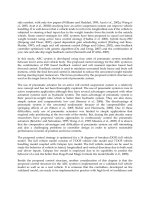
Fig. 5. Responses to desired step trajectories of classical PID and PDGC controller
PID Control, Implementation and Tuning120

With online forward kinematics available, the proposed PDGC strategy is implemented in a
real 6-DOF hydraulic parallel manipulator. The classical PID control scheme is also applied
to the parallel manipulator as benchmarking for that the classical PID control is a typical
control strategy in theory and practice, particularly in industrial hydraulic 6-DOF parallel
manipulator with heavy payload. It is should be noted that the proposed PDGC control is
an improved PID control with dynamical gravity compensation to improve the control
performance involving both steady and dynamic precision of hydraulic 6-DOF parallel
manipulator, the control strategy with gravity compensation also may be incorporated with
other advanced control scheme to derive better control performance. The classical PID gain
Kp is experimental tuned to 40, which is identical with the proposed PDGC gains. All six

DOFs step signals (Surge: 0.02m, Sway: 0.02m, Heave: 0.02m, roll: 2deg, Pitch: 2deg, Yaw:
2deg) are applied to the actual control system, respectively. Fig.5 shows the responses to the
desired step trajectory of experimental hydraulic parallel manipulator.
As shown in Fig.5, the PDGC control scheme can respond to the desired step trajectories
promptly and steadily in all DOFs. Moreover, the proposed PDGC shows superior control
performance in steady precision to those of the classical PID control along all six DOFs
directions. The maximal steady state error is 0.41mm in linear motions and 0.04deg in
angular motions under the PDGC, 1.01mm in linear motions and 0.052deg in angular
motions under the classical PID. The maximal steady state error chiefly influenced by
system gravity appeared in heave direction motion for all 6 DOFs motions under the
classical PID control, which was compensated via the proposed PDGC control, depicted in
Fig.6. Compared with the PDGC controller, the maximal steady state error in angular
motions presented in yaw direction under classical PID control is also shown in Fig.6. The
steady state error is 0.1mm in heave and 0.03deg in yaw with PDGC, 1.01mm in heave and
0.052deg in yaw with classical PID. Additionally, the responses to the step trajectories also
illustrate that the control system, both PDGC and classical PID control, is steady.

0 2 4 6 8 1
0
-0.005
0
0.005
0.01
0.015
0.02
0.025
Time /s
Maximal error in linear motions /m

Classical PID
PDGC
0 2 4 6 8 1
0
-0.5
0
0.5
1
1.5
2
Time /s
Maximal errors in angular motions /deg


Classcial PID
PDGC

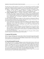
Fig. 6. The maximal errors of PDGC and classical PID controller in position and orientation

With a view of evaluating the dynamic control performance of the PDGC, the desired
sinusoidal signals are inputted to the hydraulic parallel manipulator. Under sinusoidal
inputs along six directions: surge (0.01m/1Hz), sway (0.01m/2Hz), heave (0.01m/1Hz), roll
(1deg/1Hz), pitch (1deg/2Hz), and yaw (1deg/1Hz), the trajectory tracking for the PDGC
control and the classical PID control scheme are shown in Fig. 7.

0 0.5 1 1.5 2 2.5 3
-0.01
-0.005
0
0.005

0.01
Time /s
Surge displacement q1/m


Desired trajectory
Actual under classical PID
Actual under PDGC
0 0.5 1 1.5 2
-0.01
-0.005
0
0.005
0.01
Time /s
Sway displacement q2/m


Desired trajectory
Actual under classical PID
Actual under PDGC

0 0.5 1 1.5 2
-0.01
-0.005
0
0.005
0.01
Time /s
Heave displacement q3/m

Desired trajectory
Actual under classcial PID
Actual under PDGC
0 0.5 1 1.5 2 2.5 3
-1
-0.5
0
0.5
1
Time /s
Roll displacement q4/deg


Desired trajectory
Acutal under classical PID
Actual under PDGC

0 0.5 1 1.5 2
-1
-0.5
0
0.5
1
Time /s
Pitch displacement q5/deg


Desired trajectory

Actual under classcial PID
Actual under PDGC
0 0.5 1 1.5 2 2.5 3
-2
-1.5
-1
-0.5
0
0.5
1
1.5
2
Time /s
Yaw displacement q6/deg


Desired trajectory
Actual under classical PID
Actual under PDGC

Fig. 7. Responses to desired sinusoidal trajectories of classical PID and PDGC controller
PID control with gravity compensation for hydraulic 6-DOF parallel manipulator 121

With online forward kinematics available, the proposed PDGC strategy is implemented in a
real 6-DOF hydraulic parallel manipulator. The classical PID control scheme is also applied
to the parallel manipulator as benchmarking for that the classical PID control is a typical
control strategy in theory and practice, particularly in industrial hydraulic 6-DOF parallel
manipulator with heavy payload. It is should be noted that the proposed PDGC control is
an improved PID control with dynamical gravity compensation to improve the control
performance involving both steady and dynamic precision of hydraulic 6-DOF parallel

manipulator, the control strategy with gravity compensation also may be incorporated with
other advanced control scheme to derive better control performance. The classical PID gain
Kp is experimental tuned to 40, which is identical with the proposed PDGC gains. All six
DOFs step signals (Surge: 0.02m, Sway: 0.02m, Heave: 0.02m, roll: 2deg, Pitch: 2deg, Yaw:
2deg) are applied to the actual control system, respectively. Fig.5 shows the responses to the
desired step trajectory of experimental hydraulic parallel manipulator.
As shown in Fig.5, the PDGC control scheme can respond to the desired step trajectories
promptly and steadily in all DOFs. Moreover, the proposed PDGC shows superior control
performance in steady precision to those of the classical PID control along all six DOFs
directions. The maximal steady state error is 0.41mm in linear motions and 0.04deg in
angular motions under the PDGC, 1.01mm in linear motions and 0.052deg in angular
motions under the classical PID. The maximal steady state error chiefly influenced by
system gravity appeared in heave direction motion for all 6 DOFs motions under the
classical PID control, which was compensated via the proposed PDGC control, depicted in
Fig.6. Compared with the PDGC controller, the maximal steady state error in angular
motions presented in yaw direction under classical PID control is also shown in Fig.6. The
steady state error is 0.1mm in heave and 0.03deg in yaw with PDGC, 1.01mm in heave and
0.052deg in yaw with classical PID. Additionally, the responses to the step trajectories also
illustrate that the control system, both PDGC and classical PID control, is steady.

0 2 4 6 8 1
0
-0.005
0
0.005
0.01
0.015
0.02
0.025
Time /s

Maximal error in linear motions /m


Classical PID
PDGC
0 2 4 6 8 1
0
-0.5
0
0.5
1
1.5
2
Time /s
Maximal errors in angular motions /deg


Classcial PID
PDGC

Fig. 6. The maximal errors of PDGC and classical PID controller in position and orientation

With a view of evaluating the dynamic control performance of the PDGC, the desired
sinusoidal signals are inputted to the hydraulic parallel manipulator. Under sinusoidal
inputs along six directions: surge (0.01m/1Hz), sway (0.01m/2Hz), heave (0.01m/1Hz), roll
(1deg/1Hz), pitch (1deg/2Hz), and yaw (1deg/1Hz), the trajectory tracking for the PDGC
control and the classical PID control scheme are shown in Fig. 7.

0 0.5 1 1.5 2 2.5 3
-0.01

-0.005
0
0.005
0.01
Time /s
Surge displacement q1/m


Desired trajectory
Actual under classical PID
Actual under PDGC
0 0.5 1 1.5 2
-0.01
-0.005
0
0.005
0.01
Time /s
Sway displacement q2/m


Desired trajectory
Actual under classical PID
Actual under PDGC

0 0.5 1 1.5 2
-0.01
-0.005
0
0.005

0.01
Time /s
Heave displacement q3/m


Desired trajectory
Actual under classcial PID
Actual under PDGC
0 0.5 1 1.5 2 2.5 3
-1
-0.5
0
0.5
1
Time /s
Roll displacement q4/deg


Desired trajectory
Acutal under classical PID
Actual under PDGC

0 0.5 1 1.5 2
-1
-0.5
0
0.5
1
Time /s
Pitch displacement q5/deg

Desired trajectory
Actual under classcial PID
Actual under PDGC
0 0.5 1 1.5 2 2.5 3
-2
-1.5
-1
-0.5
0
0.5
1
1.5
2
Time /s
Yaw displacement q6/deg


Desired trajectory
Actual under classical PID
Actual under PDGC

Fig. 7. Responses to desired sinusoidal trajectories of classical PID and PDGC controller
PID Control, Implementation and Tuning122

0 0.5 1 1.5 2 2.5 3
-0.01
-0.005
0

0.005
0.01
Time /s
Surge displacement q1/m


Trajectory of increased payload
Trajectory of initial payload
0 0.5 1 1.5 2
-0.01
-0.005
0
0.005
0.01
Time /s
Sway displacement q2/m


Trajectory of increased payload
Trajectory of initial payload

0 0.5 1 1.5 2 2.5 3
-0.01
-0.005
0
0.005
0.01
Time /s
Heave displacement q3/m

Trajectory of increased payload
Trajectory of initial payload
0 0.5 1 1.5 2 2.5 3
-1
-0.5
0
0.5
1
Time /s
Roll displacement q4/deg


Trajectory of increased payload
Trajectory of initial payload

0 0.5 1 1.5 2 2.5 3
-1.5
-1
-0.5
0
0.5
1
1.5
Time /s
Pitch displacement q5/deg


Trajectoy of increased payload
Trajectoy of initial payload

0 0.5 1 1.5 2 2.5 3
-2
-1.5
-1
-0.5
0
0.5
1
1.5
2
Time /s
Yaw displacement q6/deg


Trajectory of increased payload
Trajectory of initial payload

Fig. 8. Experimental results for different mass of payload

As can be deduced form Fig. 5-7, the hydraulic 6-DOF Gough-Stewart platform with PDGC,
lead the systems to the desired location with smaller steady state error neglected in large
hydraulic 6-DOF parallel manipulator, while the classical proportional plus integral plus
derivative control scheme exist large steady state errors in the system, and the PDGC
control system can implement trajectory tracking of sine wave with excellent performance in
all DOFs motions, which is better than classical proportional plus integral plus derivative
controller especially in heave direction motion.
The influence of platform load variable during the motion of 6-DOF parallel manipulator
and the robustness of the controller can be illustrated by applied the controller to the system
in the case of the platform load increase by 12%, the experimental results are shown in the
Fig.8.

Comparison of results demonstrate that the maximal amplitude fading with increased mass
of payload is 0.644dB in linear motions (q1, q2, q3), 0.154dB in angular motions (q4, q5, q6),
and it is 0.661dB in linear motions and 0.153dB in angular motions for initial mass of
payload, the maximal phase delay of PDGC controller with 112% of initial mass is 0.14rad
relative to initial mass in linear motions, while it is 0.023rad phase delay than it was with
initial mass in angular motions. Consequently, the proposed control still has excellent
performance (robustness) with incorrect mass of payload which is 112% of initial mass.
Moreover, the experimental results display that the proposed PDGC control scheme can
improve the steady precision and reduce system dynamic errors of hydraulic 6-DOF parallel
manipulator even 12% uncertainty exists in gravity, especially for 6-DOF parallel
manipulator with heavy payload.

5. Conclusions
In this paper, a proportional plus derivative control with dynamic gravity compensation is
studied for 6-DOF parallel manipulator. The system models are derived, including the
dynamics model of 6-DOF Gough-Stewart platform and actuators using Kane method and
the forward kinematics with Newton-
Raphson method and the inverse kinematics in
closed-form solution, and the hydraulic systems based on hydromechanics theory. The
control law of proportional plus derivative control with dynamic gravity compensation is
developed in the paper, the inner loop feedback controller employed dynamic gravity term,
forward kinematics and Jacobian matrix and yield servovalve currents, and the dynamics of
hydraulic systems are decoupled by local velocity compensation in inverse servosystem, the
outer loop implement the position control of actuator length. The direct estimation method
for the system states required in the proposed control based on the forward kinematics are
employed in order to realize the control scheme in the base coordinate systems instead of
the state observer with the actuator length output. The performances with respect to
stability, precision and robustness are analyzed. The theoretical analysis and simulation
results demonstrate that the proposed controller represent excellent performance for the 6-

DOF hydraulic driven Gough-Stewart platform, it is stable, the steady state errors of the
system due to gravity of the systems are converge asymptotically to zero, and the controller
reveal superexcellent robustness. Furthermore, the effective PDGC control for the hydraulic
6-DOF parallel manipulator with heavy payload is obtained in this paper; it can not only be
used in hydraulic driven 6-DOF parallel manipulator for improving classical PID control
PID control with gravity compensation for hydraulic 6-DOF parallel manipulator 123

0 0.5 1 1.5 2 2.5 3
-0.01
-0.005
0
0.005
0.01
Time /s
Surge displacement q1/m


Trajectory of increased payload
Trajectory of initial payload
0 0.5 1 1.5 2
-0.01
-0.005
0
0.005
0.01
Time /s
Sway displacement q2/m


Trajectory of increased payload

Trajectory of initial payload

0 0.5 1 1.5 2 2.5 3
-0.01
-0.005
0
0.005
0.01
Time /s
Heave displacement q3/m


Trajectory of increased payload
Trajectory of initial payload
0 0.5 1 1.5 2 2.5 3
-1
-0.5
0
0.5
1
Time /s
Roll displacement q4/deg


Trajectory of increased payload
Trajectory of initial payload

0 0.5 1 1.5 2 2.5 3
-1.5
-1

-0.5
0
0.5
1
1.5
Time /s
Pitch displacement q5/deg


Trajectoy of increased payload
Trajectoy of initial payload
0 0.5 1 1.5 2 2.5 3
-2
-1.5
-1
-0.5
0
0.5
1
1.5
2
Time /s
Yaw displacement q6/deg


Trajectory of increased payload
Trajectory of initial payload

Fig. 8. Experimental results for different mass of payload

As can be deduced form Fig. 5-7, the hydraulic 6-DOF Gough-Stewart platform with PDGC,
lead the systems to the desired location with smaller steady state error neglected in large
hydraulic 6-DOF parallel manipulator, while the classical proportional plus integral plus
derivative control scheme exist large steady state errors in the system, and the PDGC
control system can implement trajectory tracking of sine wave with excellent performance in
all DOFs motions, which is better than classical proportional plus integral plus derivative
controller especially in heave direction motion.
The influence of platform load variable during the motion of 6-DOF parallel manipulator
and the robustness of the controller can be illustrated by applied the controller to the system
in the case of the platform load increase by 12%, the experimental results are shown in the
Fig.8.

Comparison of results demonstrate that the maximal amplitude fading with increased mass
of payload is 0.644dB in linear motions (q1, q2, q3), 0.154dB in angular motions (q4, q5, q6),
and it is 0.661dB in linear motions and 0.153dB in angular motions for initial mass of
payload, the maximal phase delay of PDGC controller with 112% of initial mass is 0.14rad
relative to initial mass in linear motions, while it is 0.023rad phase delay than it was with
initial mass in angular motions. Consequently, the proposed control still has excellent
performance (robustness) with incorrect mass of payload which is 112% of initial mass.
Moreover, the experimental results display that the proposed PDGC control scheme can
improve the steady precision and reduce system dynamic errors of hydraulic 6-DOF parallel
manipulator even 12% uncertainty exists in gravity, especially for 6-DOF parallel
manipulator with heavy payload.

5. Conclusions
In this paper, a proportional plus derivative control with dynamic gravity compensation is
studied for 6-DOF parallel manipulator. The system models are derived, including the
dynamics model of 6-DOF Gough-Stewart platform and actuators using Kane method and
the forward kinematics with Newton-
Raphson method and the inverse kinematics in

closed-form solution, and the hydraulic systems based on hydromechanics theory. The
control law of proportional plus derivative control with dynamic gravity compensation is
developed in the paper, the inner loop feedback controller employed dynamic gravity term,
forward kinematics and Jacobian matrix and yield servovalve currents, and the dynamics of
hydraulic systems are decoupled by local velocity compensation in inverse servosystem, the
outer loop implement the position control of actuator length. The direct estimation method
for the system states required in the proposed control based on the forward kinematics are
employed in order to realize the control scheme in the base coordinate systems instead of
the state observer with the actuator length output. The performances with respect to
stability, precision and robustness are analyzed. The theoretical analysis and simulation
results demonstrate that the proposed controller represent excellent performance for the 6-
DOF hydraulic driven Gough-Stewart platform, it is stable, the steady state errors of the
system due to gravity of the systems are converge asymptotically to zero, and the controller
reveal superexcellent robustness. Furthermore, the effective PDGC control for the hydraulic
6-DOF parallel manipulator with heavy payload is obtained in this paper; it can not only be
used in hydraulic driven 6-DOF parallel manipulator for improving classical PID control
PID Control, Implementation and Tuning124

performance, but also can be associated with other advanced control scheme to get better
control performance and applied in other systems.

Acknowledgements
This research was supported by 921 Manned Space Project from China Academy of Space
Technology and Self-Planned Task (No.SKLRS200803B) of State Key Laboratory of Robotics
and System (HIT). The authors would like to thank CAST, HIT, Prof S. J. Li of Department
of Mechanical and Electrical Engineering, Harbin Institute of Technology, and to thank the
Editor, Associate Editors, and anonymous reviewers for their constructive comments.

Appendix A.
The 6×6 mass matrix

)
~
(
~
ΘM
, 6×6 centrifugal and Coriolis matrix
),
~
(
~
ΘΘV

, and 6×1 vector of
gravity terms
)
~
(
~
ΘG in Eqs.(4) are given by









L
m

I
I
ΘM
0
0
)
~
(
~
ep
(A.1a)











L
IΩ
ΘΘV
0
00
),
~
(

~
33

(A.1b)



T
00000)
~
(
~
gΘG (A.1c)

where I
e
is unit 3×3 matrix, I
L
is a 3×3 inertia matrix of upper platform in base coordinates
system, m
p
is the mass of upper platform.














100
010
001
e
I (A.2a)


T
p
RIRI 
L
(A.2b)

















0
0
0
xy
xz
yz



Ω (A.2c)

where I
p
is 3×3 inertia matrix relative to its symmetrical axis system, },,{diag
p zzyyxx
IIII .


Appendix B.
The mass matrix )
~
(
*
ΘM , matrix of centrifugal and Coriolis term ),
~
(
*

ΘΘV

, and gravity
terms
)
~
(
*
ΘG
in Eqs.(8) are given by




6
1
t
T
Θ
~
ai,
,ai
tcu
T
Θ
~
ai,
,ai
uc
*

])()[()
~
(
~
)
~
(
i
mm gJJgJJΘGΘG (B.1a)

Θ
~
ai,
6
1
agili
Θ
~
ai,
T*
)()
~
(
~
)
~
( JMMJΘMΘM




i
(B.1b)

}{),
~
(
~
),
~
(
ani
6
1
li
Θ
~
ai,
T*
VVJΘΘVΘΘV 

i

(B.1c)
where,

ai,
tct
ai,
tc
T

ai,
ucu
ai,
uc
T
li
JJJJM mm  (B.2a)

)(
)(
T
nn
2
agi
llI
II
M 


i
ba
l
(B.2b)

)(
~
ai,
aiuc,
~
ai,

aiuc,
T
u
aiuc,
T
li

 JJJJJV

m (B.2c)






~
ai,
T
nn
~
ai,
T
ni
2
ani
))((
)(2
JllIΘJl
II

V

i
ba
l
(B.2d)

6. References
[1] J.P. Merlet, Parallel robots, Kluwer Academic Publisher, Netherlands, 2000.
[2] J. Gallardo, J.M. Rico, A. Frisoli, D. Checcacci, M. Bergamasco, Dynamic of parallel
manipulators by means of screw theory, Mechanism and Machine Theory 38 (2003)
1113-1131
[3] A. Lopes, F. Almeida, A force-impedance controlled industrial robot using an active
robotic auxiliary device, Robotics and Computer-Integrated Manufacturing 24
(2008) 299-309.
[4] Y.N. Wu, C. Gosselin, Design of reactionless 3-DOF and 6-DOF parallel manipulators using
parallelepiped mechanisms, IEEE Transactions on Robotics 21 (5) (2005) 821-833
[5] D. Stewart, A platform with six degree of freedom: A new form of mechanical linage
which enables a platform to move simultaneously in six degree of freedom
developed by Elliot-Automation, Aircraft Engineering and Aerospace Technology
38 (4) (1965) 30-35.
[6] J.P. Merlet, Parallel manipulators: state of the art and perspectives, Advanced Robotics 8
(6) (1994) 589-596.
[7] K.H. Hunt, Structural kinematics of in-parallel-actuated robot-arms, ASME Journal of
Mechanisms, Transmissions and Automation in Design 105(4) (1983) 705-712.
PID control with gravity compensation for hydraulic 6-DOF parallel manipulator 125

performance, but also can be associated with other advanced control scheme to get better
control performance and applied in other systems.

Acknowledgements
This research was supported by 921 Manned Space Project from China Academy of Space
Technology and Self-Planned Task (No.SKLRS200803B) of State Key Laboratory of Robotics
and System (HIT). The authors would like to thank CAST, HIT, Prof S. J. Li of Department
of Mechanical and Electrical Engineering, Harbin Institute of Technology, and to thank the
Editor, Associate Editors, and anonymous reviewers for their constructive comments.

Appendix A.
The 6×6 mass matrix
)
~
(
~
ΘM
, 6×6 centrifugal and Coriolis matrix
),
~
(
~
ΘΘV

, and 6×1 vector of
gravity terms
)
~
(
~
ΘG in Eqs.(4) are given by








L
m
I
I
ΘM
0
0
)
~
(
~
ep
(A.1a)












L
IΩ
ΘΘV
0
00
),
~
(
~
33

(A.1b)



T
00000)
~
(
~
gΘG (A.1c)

where I
e
is unit 3×3 matrix, I
L
is a 3×3 inertia matrix of upper platform in base coordinates
system, m
p

is the mass of upper platform.













100
010
001
e
I (A.2a)


T
p
RIRI 
L
(A.2b)

















0
0
0
xy
xz
yz



Ω (A.2c)

where I
p
is 3×3 inertia matrix relative to its symmetrical axis system, },,{diag
p zzyyxx
III

I .

Appendix B.
The mass matrix )
~
(
*
ΘM , matrix of centrifugal and Coriolis term ),
~
(
*
ΘΘV

, and gravity
terms
)
~
(
*
ΘG
in Eqs.(8) are given by




6
1
t
T
Θ

~
ai,
,ai
tcu
T
Θ
~
ai,
,ai
uc
*
])()[()
~
(
~
)
~
(
i
mm gJJgJJΘGΘG (B.1a)

Θ
~
ai,
6
1
agili
Θ
~
ai,

T*
)()
~
(
~
)
~
( JMMJΘMΘM



i
(B.1b)

}{),
~
(
~
),
~
(
ani
6
1
li
Θ
~
ai,
T*
VVJΘΘVΘΘV 


i

(B.1c)
where,

ai,
tct
ai,
tc
T
ai,
ucu
ai,
uc
T
li
JJJJM mm  (B.2a)

)(
)(
T
nn
2
agi
llI
II
M 



i
ba
l
(B.2b)

)(
~
ai,
aiuc,
~
ai,
aiuc,
T
u
aiuc,
T
li

 JJJJJV

m (B.2c)






~
ai,
T

nn
~
ai,
T
ni
2
ani
))((
)(2
JllIΘJl
II
V

i
ba
l
(B.2d)

6. References
[1] J.P. Merlet, Parallel robots, Kluwer Academic Publisher, Netherlands, 2000.
[2] J. Gallardo, J.M. Rico, A. Frisoli, D. Checcacci, M. Bergamasco, Dynamic of parallel
manipulators by means of screw theory, Mechanism and Machine Theory 38 (2003)
1113-1131
[3] A. Lopes, F. Almeida, A force-impedance controlled industrial robot using an active
robotic auxiliary device, Robotics and Computer-Integrated Manufacturing 24
(2008) 299-309.
[4] Y.N. Wu, C. Gosselin, Design of reactionless 3-DOF and 6-DOF parallel manipulators using
parallelepiped mechanisms, IEEE Transactions on Robotics 21 (5) (2005) 821-833
[5] D. Stewart, A platform with six degree of freedom: A new form of mechanical linage
which enables a platform to move simultaneously in six degree of freedom

developed by Elliot-Automation, Aircraft Engineering and Aerospace Technology
38 (4) (1965) 30-35.
[6] J.P. Merlet, Parallel manipulators: state of the art and perspectives, Advanced Robotics 8
(6) (1994) 589-596.
[7] K.H. Hunt, Structural kinematics of in-parallel-actuated robot-arms, ASME Journal of
Mechanisms, Transmissions and Automation in Design 105(4) (1983) 705-712.
PID Control, Implementation and Tuning126

[8] W.Q.D. Do, D.C.H. Yang, Inverse dynamic analysis and simulation of a platform type of
robot, Journal of Robotic Systems 5 (1988) 209-227.

[9] M. Honegger, R. Brega, G. Schweizer, Application of a nonlinear adaptive controller to a 6
dof parallel manipulator, In Proceeding of the 2000 IEEE International Conference on
Robotics and Automation, San Francisco, CA, USA, (2000) pp. 1930-1935.
[10] D.H. Kim, J.Y. Kang, K-II. Lee, Robust tracking control design for a 6 DOF parallel
manipulator, Journal of Robotics Systems 17(10) (2000) 527-547.
[11] C.C. Nguyen, S.S. Antrazi, Z.L. Zhou, C.E. Campbell, Adaptive control of a Stewart
platform-based manipulator, Journal of Robotics Systems 10(5) (1992) 657-687.
[12] H.S. Kim, Y.M. Cho, K-II. Lee, Robust nonlinear task space control for a 6 DOF parallel
manipulator, Automatica 41 (2005) 1591-1600.
[13] Y. Ting, Y.S. Chen, H.C. Jar, Modeling and control for a Gough-Stewart platform CNC
machine, Journal of Robotics System 21(11) (2004) 609-623.
[14] J.L. Chen, W.D. Chang, Feedback linearization control of a two-link robot using a multi-
crossover genetic algorithm, Expert Systems with Applications 36 (2009) 4154-4159.
[15] K.J. Astrom, T. Hagglund. PID Controllers: Theory, Design, and Tuning. Instrument
Society of America: NC, 1995.
[16] Y.X Su, B.Y. Duan, C.H. Zheng, Y.F. Zhang, G.D. Chen, J.W. Mi, Disturbance-rejection
high-precision motion control of a Stewart platform, IEEE Transactions on Control
Systems Technology 12(3) (2004) 364-374.
[17] E. Burdet, M. Honegger, A. Codourey, Controllers with desired dynamic compensation and

their implementation on a 6 DOF parallel manipulator, Proceeding of the 2000
IEEE/RSJ International Conference on Intelligent Robots and Systems, 2000, pp. 39-45.
[18] J.R. Noriega, H. Wang, A direct adaptive neural-network control for unknown nonlinear
systems and its application, IEEE Transactions on Neural Networks 9 (1) (1998) 27-34.
[19] N.I. Kim, C.W. Lee, High speed tracking control of Stewart platform manipulator via
enhanced sliding mode control, In Proceeding of the 1998 IEEE Conference on
Robotics and Automation, Leuven, Belgium, (1998) pp. 2716-2721.
[20] I. Cervantes, J.A. Ramirez, On the PID tracking control of robot manipulators, Systems
& Control Letters 42 (2001) 37-46.
[21] I. Davliskos, E. Papadopoulous, Model-based control of 6-DOF electrohydraulic parallel
manipulator platform, Mechanism and Machine Theory 43 (2008) 1385-1400.
[22] F. Behi, Kinematic analysis for a six-degree-of-freedom 3-PRPS parallel mechanism,
IEEE Journal of Robotics and Automation 4(5) (1988) 561-565.
[23] D.M. Ku, Direct displacement analysis of a Stewart platform mechanism. Mechanism
and Machine Theory 34 (1999) 453-465.
[24] B. Dasgupta, T.S. Mruthyunjaya, A Newton-Euler formulation for the inverse dynamics
of the Stewart platform manipulator, Mechanism and Machine Theory 33(8) (1998)
1135-1152.
[25] S.H. Koekebakker, Model based control of a flight simulator motion system. Ph.D
Thesis. Netherlands: Delft University of Technology, 2001.
[26] H.E. Merrit, Hydraulic Control Systems, Wiley, 1967.
[27] D. Rowell, D.N. Wormley, System Dynamics: An Introduction, Prentice Hall, 1997.
[28] R. Gorez, Globally stable PID-like control of mechanical systems, Systems & Control
Letters 38 (1999) 61-72.
[29] C.F. Yang, J.F. He, J.W. Han, X.C. Liu, Real-time state estimation for spatial six-degree-
of-freedom linearly actuated parallel robots. Mechatronics 19(6) (2009) 1026-1033.
Sampled-Data PID Control and Anti-aliasing Filters 127
Sampled-Data PID Control and Anti-aliasing Filters
Marian J. Blachuta and Rafal T. Grygiel
0

Sampled-Data PID Control and Anti-aliasing Filters
*
Marian J. Blachuta and Rafal T. Grygiel
Department of Automatic Control, Silesian University of Technology
Poland
1. Introduction
Consider a typical configuration of the sampled-data control system. It consists of the plant
to be controlled, a sampler, a discrete-time controller and a zero-order hold. Disturbance can
be seen as an integral part of the plant so that the plant is characterized by the control path re-
sponsible for control signal influence on the output and the disturbance. The system output is
usually sensed by sensors whose output signal can be corrupted by noise. Sometimes analog
filters are put between the analog sensor output signal and sampler. In the control literature
Analog Filter
h
Controller
ZOH
Disturbance
Plant
Noise
Analog Filter
h
Controller
ZOH
Disturbance
Plant
Nois
e
Control
Path
Fig. 1. General control system diagram

(Åström and Wittenmark, 1997; Feuer and Goodwin, 1996) strong belief is expressed, that fil-
ters are necessary prior to sampling to guarantee correct digital signal processing and control.
This belief is usually supported by heuristic speculations based on Shannon-Kotelnikov Re-
construction Theorem, e.g. (Jerri, 1977), which states that in order to reconstruct the signal
s
(t) from its samples s(ih), −∞ < i < ∞, the sampling frequency should be at least twice the
highest frequency component in the signal. Since the spectra of physical signals often stretch
on infinite frequency range, this gives rise to the idea of so called anti-aliasing filters that cut
off the portion of frequency spectrum lying outside the region determined by that theorem.
*
This work has been granted by the Polish Ministry of Science and Higher Education from funds for
years 2008-2011
6
PID Control, Implementation and Tuning128
It should, however, be stressed that no proofs are available concerning the necessity of anti-
aliasing filters in sampled-data systems, and no statements can be found with regard to the
consequences of the lack of such filters.
Anti-aliasing filters usually take the form of Butterworth filters whose cutoff frequency equals
to the so called Nyquist frequency ω
N
= π/h, which is depending solely on sampling period
h. As an alternative, so called integrating or averaging samplers are considered (Blachuta &
Grygiel, 2008a;b; Feuer and Goodwin, 1996; Goodwin et al., 2001; Steinway and Melsa, 1971;
Shats and Shaked, 1989).
In (Blachuta & Grygiel, 2008a;b) we studied the impact of antialiasing filters for pure signal
processing, while in (Blachuta & Grygiel, 2009b) the context of discrete-time LQG control was
discussed. The statement was made, that there is no reason for using them in the noiseless
case, and practically they find no use in the case of noisy measurements. The best results in
the latter case are obtained when the continuous-time output is passed through a continuous-
time Kalman filter, which depends rather on disturbance and noise characteristics than the

sampling period, before being sampled. Similar results were observed in PID control systems
(Blachuta & Grygiel, 2009a;b;c)and (Blachuta & Grygiel, 2010)
In this chapter we summarize these results and compare them with LQG minimum-variance
benchmark control using simple, but representative examples.
2. Analog part of the system
2.1 Plant, disturbance and noise model
The model of system displayed in Fig. 1 is presented in Fig. 2, where K
c
(s) is the transfer
function of control path of the plant, while K
d
(s) and K
n
(s) represent filters forming stochastic
disturbance and noise, respectively. K
f
(s) stands for a continuous-time filter.


d
t




u t
 
c
y t



d t


c
K
s


d
K
s


n t


n
t


 
n
K
s
h
LQG / PID
ZOH



s t


y t
i
u
i
z


f
K
s
Fig. 2. Control system
The entire continuous-time system can be modeled in state-space as follows:
˙x
(t) = Ax(t) + bu(t) + C
˙
ξ(t), (1)
y
(t) = d

y
x(t), (2)
s
(t) = d

s
x(t), (3)
z

(t) = d

x(t), (4)
where:
A
=




A
c
0 0 0
0 A
d
0 0
0 0 A
n
0
b
f
d

c
b
f
d

d
b

f
d

n
A
f




, C
=




0 0
c
d
0
0 c
n
0 0




,
b
=





b
c
0
0
0




, d
y
=




d
c
d
d
0
0





, d
s
=




d
c
d
d
d
n
0




, d
=




0
0
0
d
f





,
x
(t) =




˙x
c
(t)
˙x
d
(t)
˙x
n
(t)
˙x
f
(t)




,
˙
ξ
(t) =


˙
ξ
d
(t)
˙
ξ
n
(t)

.
Processes
˙
ξ
d
(t) and
˙
ξ
n
(t) are independent continuous-time white noises with zero means and
covariance functions defined as unit Dirac pulse functions, i.e.:
E
[
˙
ξ
d
(t)] = 0, E [
˙
ξ
d

(t)
˙
ξ
d
(τ)] = δ(t −τ); (5)
E
[
˙
ξ
n
(t)] = 0, E [
˙
ξ
n
(t)
˙
ξ
n
(τ)] = δ(t −τ). (6)
2.2 Analog Filters
In the paper two types of filters are considered: Butterworth filter as the anti-aliasing filter, as
well as a continuous-time Kalman filter as a filter based on signals spectra.
2.2.1 Butterworth Filter
Transfer function of the Butterworth filter has the form:
K
f
(
s
)
=

1
B
n

s
ω
o

, (7)
where B
n
(
∗
)
is the n
th
-degree Butterworth’s polynomial and ω
o
is called the cutoff frequency.
In this paper ω
o
will be assumed as Nyquist frequency ω
o
= ω
N
=
π
h
. The first Butterworth’s
polynomials are definded as follows:

B
1
(
x
)
=
x + 1; B
2
(
x
)
=
x
2
+
√
2 · x + 1. (8)
Sampled-Data PID Control and Anti-aliasing Filters 129
It should, however, be stressed that no proofs are available concerning the necessity of anti-
aliasing filters in sampled-data systems, and no statements can be found with regard to the
consequences of the lack of such filters.
Anti-aliasing filters usually take the form of Butterworth filters whose cutoff frequency equals
to the so called Nyquist frequency ω
N
= π/h, which is depending solely on sampling period
h. As an alternative, so called integrating or averaging samplers are considered (Blachuta &
Grygiel, 2008a;b; Feuer and Goodwin, 1996; Goodwin et al., 2001; Steinway and Melsa, 1971;
Shats and Shaked, 1989).
In (Blachuta & Grygiel, 2008a;b) we studied the impact of antialiasing filters for pure signal
processing, while in (Blachuta & Grygiel, 2009b) the context of discrete-time LQG control was

discussed. The statement was made, that there is no reason for using them in the noiseless
case, and practically they find no use in the case of noisy measurements. The best results in
the latter case are obtained when the continuous-time output is passed through a continuous-
time Kalman filter, which depends rather on disturbance and noise characteristics than the
sampling period, before being sampled. Similar results were observed in PID control systems
(Blachuta & Grygiel, 2009a;b;c)and (Blachuta & Grygiel, 2010)
In this chapter we summarize these results and compare them with LQG minimum-variance
benchmark control using simple, but representative examples.
2. Analog part of the system
2.1 Plant, disturbance and noise model
The model of system displayed in Fig. 1 is presented in Fig. 2, where K
c
(s) is the transfer
function of control path of the plant, while K
d
(s) and K
n
(s) represent filters forming stochastic
disturbance and noise, respectively. K
f
(s) stands for a continuous-time filter.


d
t




u t

 
c
y t


d t


c
K
s


d
K
s


n t


n
t


 
n
K
s
h

LQG / PID
ZOH


s t


y t
i
u
i
z


f
K
s
Fig. 2. Control system
The entire continuous-time system can be modeled in state-space as follows:
˙x
(t) = Ax(t) + bu(t) + C
˙
ξ(t), (1)
y
(t) = d

y
x(t), (2)
s
(t) = d


s
x(t), (3)
z
(t) = d

x(t), (4)
where:
A
=




A
c
0 0 0
0 A
d
0 0
0 0 A
n
0
b
f
d

c
b
f

d

d
b
f
d

n
A
f




, C
=




0 0
c
d
0
0 c
n
0 0





,
b
=




b
c
0
0
0




, d
y
=




d
c
d
d
0
0





, d
s
=




d
c
d
d
d
n
0




, d
=




0
0

0
d
f




,
x
(t) =




˙x
c
(t)
˙x
d
(t)
˙x
n
(t)
˙x
f
(t)





,
˙
ξ
(t) =

˙
ξ
d
(t)
˙
ξ
n
(t)

.
Processes
˙
ξ
d
(t) and
˙
ξ
n
(t) are independent continuous-time white noises with zero means and
covariance functions defined as unit Dirac pulse functions, i.e.:
E
[
˙
ξ
d

(t)] = 0, E [
˙
ξ
d
(t)
˙
ξ
d
(τ)] = δ(t −τ); (5)
E
[
˙
ξ
n
(t)] = 0, E [
˙
ξ
n
(t)
˙
ξ
n
(τ)] = δ(t −τ). (6)
2.2 Analog Filters
In the paper two types of filters are considered: Butterworth filter as the anti-aliasing filter, as
well as a continuous-time Kalman filter as a filter based on signals spectra.
2.2.1 Butterworth Filter
Transfer function of the Butterworth filter has the form:
K
f

(
s
)
=
1
B
n

s
ω
o

, (7)
where B
n
(
∗
)
is the n
th
-degree Butterworth’s polynomial and ω
o
is called the cutoff frequency.
In this paper ω
o
will be assumed as Nyquist frequency ω
o
= ω
N
=

π
h
. The first Butterworth’s
polynomials are definded as follows:
B
1
(
x
)
=
x + 1; B
2
(
x
)
=
x
2
+
√
2 · x + 1. (8)
PID Control, Implementation and Tuning130
2.2.2 Kalman Filter
Kalman filter is the one that provides the best noise filtering under assumptions of our model.
Since the noise added to the measured output is not white, the classical Kalman filter for
a system consisting of disturbance and noise becomes singular. One way to overcome the
problem is to replace the continuous-time filter with a discrete-time one working at a high
enough sampling frequency 1/h
f
. The output of such filter could be re-sampled at lower

frequency if necessary.
Very often the power spectrum S
n
(ω) of noise n(t), defined by transfer function K
n
(s), is
much wider than that of the signal of interest y
(t). In such case it can be modeled as white
noise n
(t)
E [n(t)] = 0, E [n(t)n(τ)] = η
2
δ(t − τ); (9)
with constant spectral density η
2
independent of frequency ω. The model of disturbances is
then simplified to
˙x
d
(t) = A
d
x
d
(t) + c
d
˙
ξ
d
(t), (10)
y

dn
(t) = d

d
x
d
(t) + η
˙
ξ
n
(t), (11)
with
η
= |K
n
(0)| = |d

n
A
−1
n
c
n
| (12)
The continuous-time Kalman filter is then defined by:
˙x
f
(t) = A
d
x

f
(t) + k
f
c

y
dn
(t) −d

d
x
f
(t)

(13)
where:
k
f
c
=
P d
d
η
2
; A
d
P + P A

d
−

P d
d
d

d
P
η
2
+ c
d
c

d
= 0. (14)
We use this filter in the system to pass the signal y
2
(t) through it, i.e. we substitute y
dn
(t) =
y
2
(t) and receive z(t) = d

d
x
f
(t)
Since only a rough characterization of noise is required and filter equations are of lower order
equal to the order of disturbance model, analog filtering is greatly simplified.
3. Control algorithms

The aim of the control system is to keep the output of the system close to the reference value
y
r
(t) = 0, i.e. to make the error e(t) = y
r
(t) − y( t) small. Since standard deviation is a
good measure of the expected magnitude, the quality of the control systems will be assessed
based on standard deviation of output and control signals. To this end, appropriate variations
should be calculated.
3.1 PID controller
Discrete-time PID controller defined by transfer function:
K
reg
(z) =
U(z)
E(z)
=
k
P

1
+
h
T
I
z
z −1
+
T
D

h
z
−1
z

(15)
can be presented in the state-space form, assuming e
i
= −z
i
, as follows:
x
r
i
+1
= F
r
x
r
i
−g
r
z
i
, (16)
u
i
= d

r

x
r
i
−e
r
z
i
, (17)
P k
P
=
T
k
·L
– –
PI k
P
= 0.9
T
k
·L
T
I
= 3.33 · L –
PID k
P
= 1.2
T
k
·L

T
I
= 2 · L T
D
= 0.5 · L
Table 1. QDR PID controller settings
where:
F
r
=

1 0
0 0

, g
r
=

1
1

, d
r
=

k
P
h
T
I

−k
P
T
D
h

, e
r
= k
p

1
+
h
T
I
+
T
D
h

(18)
3.1.1 QDR controller settings
There are several methods to find continuous-time PID controller settings. Perhaps the
simplest one is the so called QDR (Quarter Decay Ratio) method, which is based on lag-
delay approximation of the plant. We adapt this method to sampled-data controller using
a continuous-time approximation of the discrete-time system consisting of ZOH, plant, fil-
ter and sampler. Moreover, a lag-delay approximation G
OL
(s) of the control path including

respective filter, K
OL
(s) = K
c
(s)K
f
(s), is used.
G
OL
(s) =
k
Ts
+ 1
e
−sτ
. (19)
The parameters of G
OL
(s) can be determined by several methods based on the step response
of K
OL
(s). One of them, called "two points method", relies on two time instants, t
1
and t
2
, at
which the step response reaches the values 63.2% and 28.3% of the steady state, respectively.
We then have:
T
= 1.5

(
t
1
−t
2
)
, τ = t
1
− T. (20)
Then the QDR settings (Goodwin et al., 2001) are taken from Table 1 where L accounts for
ZOH and sampler as follows:
L
= τ +
h
2
, (21)
which corresponds to the h/2 delay approximation of ZOH.
3.1.2 Optimal PID controller
QDR controller settings do not depend on disturbance and noise characteristics. Therefore
optimal controllers settings ˆp
=

ˆ
k
P
ˆ
T
j
I
ˆ

T
j
D


will be chosen as the ones minimizing the
output variance of the controlled system:
ˆp
= arg min
p
var {y
i
} (22)
where the variance var
{y
i
} is determined by the formuale in (24) - (28) that take disturbance
and noise characteristics into account. Denoting ˆp
j
=

ˆ
k
j
P
ˆ
T
j
I
ˆ

T
j
D


at j-th stage of the
minimization procedure, the computation stops when:
 ˆp
j
− ˆp
j−1
 < ε where ε = 0.01 (23)
Sampled-Data PID Control and Anti-aliasing Filters 131
2.2.2 Kalman Filter
Kalman filter is the one that provides the best noise filtering under assumptions of our model.
Since the noise added to the measured output is not white, the classical Kalman filter for
a system consisting of disturbance and noise becomes singular. One way to overcome the
problem is to replace the continuous-time filter with a discrete-time one working at a high
enough sampling frequency 1/h
f
. The output of such filter could be re-sampled at lower
frequency if necessary.
Very often the power spectrum S
n
(ω) of noise n(t), defined by transfer function K
n
(s), is
much wider than that of the signal of interest y
(t). In such case it can be modeled as white
noise n

(t)
E [n(t)] = 0, E [n(t)n(τ)] = η
2
δ(t − τ); (9)
with constant spectral density η
2
independent of frequency ω. The model of disturbances is
then simplified to
˙x
d
(t) = A
d
x
d
(t) + c
d
˙
ξ
d
(t), (10)
y
dn
(t) = d

d
x
d
(t) + η
˙
ξ

n
(t), (11)
with
η
= |K
n
(0)| = |d

n
A
−1
n
c
n
| (12)
The continuous-time Kalman filter is then defined by:
˙x
f
(t) = A
d
x
f
(t) + k
f
c

y
dn
(t) −d


d
x
f
(t)

(13)
where:
k
f
c
=
P d
d
η
2
; A
d
P + P A

d
−
P d
d
d

d
P
η
2
+ c

d
c

d
= 0. (14)
We use this filter in the system to pass the signal y
2
(t) through it, i.e. we substitute y
dn
(t) =
y
2
(t) and receive z(t) = d

d
x
f
(t)
Since only a rough characterization of noise is required and filter equations are of lower order
equal to the order of disturbance model, analog filtering is greatly simplified.
3. Control algorithms
The aim of the control system is to keep the output of the system close to the reference value
y
r
(t) = 0, i.e. to make the error e(t) = y
r
(t) − y( t) small. Since standard deviation is a
good measure of the expected magnitude, the quality of the control systems will be assessed
based on standard deviation of output and control signals. To this end, appropriate variations
should be calculated.

3.1 PID controller
Discrete-time PID controller defined by transfer function:
K
reg
(z) =
U(z)
E(z)
=
k
P

1
+
h
T
I
z
z
−1
+
T
D
h
z
−1
z

(15)
can be presented in the state-space form, assuming e
i

= −z
i
, as follows:
x
r
i
+1
= F
r
x
r
i
−g
r
z
i
, (16)
u
i
= d

r
x
r
i
−e
r
z
i
, (17)

P k
P
=
T
k·L
– –
PI k
P
= 0.9
T
k·L
T
I
= 3.33 · L –
PID k
P
= 1.2
T
k·L
T
I
= 2 · L T
D
= 0.5 · L
Table 1. QDR PID controller settings
where:
F
r
=


1 0
0 0

, g
r
=

1
1

, d
r
=

k
P
h
T
I
−k
P
T
D
h

, e
r
= k
p


1
+
h
T
I
+
T
D
h

(18)
3.1.1 QDR controller settings
There are several methods to find continuous-time PID controller settings. Perhaps the
simplest one is the so called QDR (Quarter Decay Ratio) method, which is based on lag-
delay approximation of the plant. We adapt this method to sampled-data controller using
a continuous-time approximation of the discrete-time system consisting of ZOH, plant, fil-
ter and sampler. Moreover, a lag-delay approximation G
OL
(s) of the control path including
respective filter, K
OL
(s) = K
c
(s)K
f
(s), is used.
G
OL
(s) =
k

Ts + 1
e
−sτ
. (19)
The parameters of G
OL
(s) can be determined by several methods based on the step response
of K
OL
(s). One of them, called "two points method", relies on two time instants, t
1
and t
2
, at
which the step response reaches the values 63.2% and 28.3% of the steady state, respectively.
We then have:
T
= 1.5
(
t
1
−t
2
)
, τ = t
1
− T. (20)
Then the QDR settings (Goodwin et al., 2001) are taken from Table 1 where L accounts for
ZOH and sampler as follows:
L

= τ +
h
2
, (21)
which corresponds to the h/2 delay approximation of ZOH.
3.1.2 Optimal PID controller
QDR controller settings do not depend on disturbance and noise characteristics. Therefore
optimal controllers settings ˆp
=

ˆ
k
P
ˆ
T
j
I
ˆ
T
j
D


will be chosen as the ones minimizing the
output variance of the controlled system:
ˆp
= arg min
p
var {y
i

} (22)
where the variance var
{y
i
} is determined by the formuale in (24) - (28) that take disturbance
and noise characteristics into account. Denoting ˆp
j
=

ˆ
k
j
P
ˆ
T
j
I
ˆ
T
j
D


at j-th stage of the
minimization procedure, the computation stops when:
 ˆp
j
− ˆp
j−1
 < ε where ε = 0.01 (23)

PID Control, Implementation and Tuning132
In the above, Powell method of extremum seeking, amended with a procedure determining
the range of stable values of parameters at each direction, can be used. The parameters result-
ing from QDR tuning can then be chosen as an initial guess.
3.1.3 PID Control System Assessment
The output and control variances are as follows:
σ
2
y
= var {y
i
} = d

y
V
p
d
y
, (24)
σ
2
u
= var {u
i
} = d

r
V
r
d

r
+ e
r
d

V
p
de
r
−d

r
V
rp
de
r
−e
r
d

V
pr
d
r
, (25)
where the covariance matrix V
V
= E

x

i
x
r
i


x

i
x
r
i


=

V
p
i
V
pr
i
V
rp
i
V
r
i

(26)

is a solution of
V
= ΦV Φ

+ ΛW Λ

(27)
with
Φ
=

(
F −ge
r
d

)
gd

r
−g
r
d

F
r

, Λ
=


I
0

(28)
3.2 MV LQG control law
The best control accuracy is achieved when using the optimal Minimum-Variance sampled-
data LQG controller which will be used as a benchmark to assess PID control quality.
3.2.1 Controller
LQG control problem with a continuous performance index J is formulated, where
J
= lim
N→∞
E
1
Nh
Nh

0

y
2
(t) + λu
2
(t)

dt. (29)
Setting λ
= 0 defines a MV sampled-data LQG problem. Since noise influences only state
estimate ˆx
i|i

and not the control law, being itself a linear function of ˆx
i|i
the above sampled
data control problem can be reformulated as follows.
The problem defined by modulation equation
u(t) = u
i
, for t ∈ (ih, ih + h], i = 0, 1, . . . , (30)
state equation
˙x
p
(t) = A
p
x
p
(t) + b
p
u(t) + c
p
˙
ξ
(t), (31)
y
(t) = d

p
x
p
(t), (32)
where:

A
p
=

A
c
0
0 A
d

, b
p
=

b
c
0

, c
p
=

0
c
d

,
d
p
=


d
c
d
d

, x
p
(t) =

x
c
(t)
x
d
(t)

,
˙
ξ
(t) =
˙
ξ
d
(t),
and feedback signal z
i
, is equivalent with the following discrete-time problem
x
p

i
+1
= F
p
x
p
i
+ g
p
u
i
+ w
p
i
, (33)
z
i
= d

p
x
p
i
, (34)
J
= lim
N→∞
E
1
N

N−1
∑
i=0

x
p
i
Q
1
x
p
i
+ 2x
p
i
q
12
u
i
+ q
2
u
2
i
+ q
w

, (35)
where
Q

1
=
1
h
h

0
F

p
(τ)M F
p
(τ)dτ, M = d
p
d

p
,
q
12
=
1
h
h

0
F

p
(τ)M g

p
(τ)dτ,
q
2
=
1
h
h

0
g

p
(τ)M g
p
(τ)dτ + λ,
q
w
= d

p



h

0
τ

0

F
p
(τ − s)c
p
c

p
F

p
(τ − s)dsdτ



d
p
,
F
p
(τ) = e
A
A
A
p
τ
, F
p
= F
p
(h), (36)

g
p
(τ) =
τ

0
e
A
A
A
p
ν
b
p
dν, g
p
= g
p
(h) (37)
and w
p
i
is a zero mean vector Gaussian noise with E {w
p
i
w
p
i
} = W
p

, and
W
p
=
h

0
e
A
A
A
p
s
c
p
c

p
e
A
A
A

p
s
ds. (38)
Vectors x
p
0
and w

p
i
are independent for all i ≥ 0. The optimal control law minimizing the
performance index (35) for the discrete stochastic system (33)-(34) is a linear function
u
i
= −k

x
ˆx
p
i
|i
, (39)
where ˆx
p
i
|i
denotes the Kalman filter estimate of x
p
i
based on available information up to and
including i from (47)-(48).The feedback gain k
x
,
k

x
=
q

12
+ F

p
Kg
p
q
2
+ g

p
Kg
p
(40)
depends on the positive definite solution K of the following algebraic Riccati equation:
K
= Q
1
+ F

p
KF
p
−
(
q
12
+ F

p

Kg
p
)(q
12
+ F

p
Kg
p
)

q
2
+ g

p
Kg
p
.