Robust Control Theory and Applications Part 4 pptx

Robust H
∞
Tracking Control of Stochastic Innate Immune System Under Noises

107
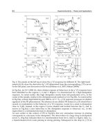
0 1 2 3 4 5 6 7 8
0
1
2
3
4
5
6
The lethal case
Time unit
Concentration
x
1
Pathogens
x
2
Immune cells
x
3
Antibodies
x
4
Organ
Organ failure
Organ survival

Fig. 6. The uncontrolled stochastic immune responses (lethal case) in (33) are shown to
increase the level of pathogen concentration at the beginning of the time period. In this case,
we try to administrate a treatment after a short period of pathogens infection. The cutting
line (black dashed line) is an optimal time point to give drugs. The organ will survive or fail
based on the organ health threshold (horizontal dotted line) [x
4
<1: survival, x
4
>1: failure].
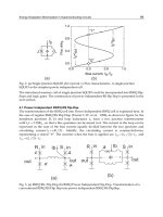
To minimize the design effort and complexity for this nonlinear innate immune system in
(33), we employ the T-S fuzzy model to construct fuzzy rules to approximate nonlinear
immune system with the measurement output
3
y and
4
y
as premise variables.
Plant Rule i:
If
3
y is
1i
F and
4
y
is
2i
F , then
() () () (), 1,2,3, ,
i

xt xt ut Dwt i L=++ =AB



() () ()yt Cxt nt=+
To construct the fuzzy model, we must find the operating points of innate immune
response. Suppose the operating points for
3
y
are at
31
0.333y =− ,
32
1.667y = , and
33
3.667y = . Similarly, the operating points for
4
y
are at
41
0y
=
,
42
1y
=
, and
43
2y = . For
the convenience, we can create three triangle-type membership functions for the two

premise variables as in Fig. 7 at the operating points and the number of fuzzy rules is 9L = .
Then, we can find the fuzzy linear model parameters
i
A in the Appendix D as well as other
parameters
B , C and D . In order to accomplish the robust H
∞
tracking performance, we
should adjust a set of weighting matrices
1
Q and
2
Q in (8) or (9) as
1
0.01 0 0 0
00.010 0
0 0 0.01 0
0000.01
Q
⎡
⎤
⎢
⎥
⎢
⎥
=
⎢
⎥
⎢
⎥

⎣
⎦
,
2
0.01000
00.010 0
0 0 0.01 0
0000.01
Q
⎡
⎤
⎢
⎥
⎢
⎥
=
⎢
⎥
⎢
⎥
⎣
⎦
.
After specifying the desired reference model, we need to solve the constrained optimization
problem in (32) by employing Matlab Robust Control Toolbox. Finally, we obtain the
feasible parameters 40
γ
= and
1
0.02γ=

, and a minimum attenuation level
2
0
0.93ρ= and a
Robust Control, Theory and Applications

108
common positive-definite symmetric matrix P with diagonal matrices
11
P ,
22
P and
33
P as
follows
11
0.23193 -1.5549e-4 0.083357 -0.2704
-1.5549e-4 0.010373 -1.4534e-3 -7.0637e-3
0.083357 -1.4534e-3 0.33365 0.24439
-0.2704 -7.0637e-3 0.24439 0.76177
P
⎡
⎤
⎢
⎥
⎢
⎥
=
⎢
⎥

⎢
⎥
⎣
⎦
,
22
0.0023082 9.4449e-6 -5.7416e-5 -5.0375e-6
9.4449e-6 0.0016734 2.4164e-5 -1.8316e-6
-5.7416e-5 2.4164e-5 0.0015303 5.8989e-6
-5.0375e-6 -1.8316e-6 5.8989e-6 0.0015453
P
⎡
⎤
⎢
⎥
⎢
⎥
=
⎢
⎥
⎢
⎥
⎣
⎦

33
1.0671 -1.0849e-5 3.4209e-5 5.9619e-6
-1.0849e-5 1.9466 -1.4584e-5 1.9167e-6
3.4209e-5 -1.4584e-5 3.8941 -3.2938e-6
5.9619e-6 1.9167e-6 -3.2938e-6 1.4591

P
⎡
⎤
⎢
⎥
⎢
⎥
=
⎢
⎥
⎢
⎥
⎣
⎦

The control gain
j
K
and the observer gain
i
L can also be solved in the Appendix D.

1
3
y
31
y
32
y
33

y
1
4
y
41
y
42
y
43
y

Fig. 7. Membership functions for two premise variables
3
y
and
4
y
.
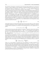
Figures 8-9 present the robust H
∞
tracking control of stochastic immune system under the
continuous exogenous pathogens, environmental disturbances and measurement noises.
Figure 8 shows the responses of the uncontrolled stochastic immune system under the initial
concentrations of the pathogens infection. After the one time unit (the black dashed line), we
try to provide a treatment by the robust H
∞
tracking control of pathogens infection. It is seen
that the stochastic immune system approaches to the desired reference model quickly. From
the simulation results, the tracking performance of the robust model tracking control via T-S
fuzzy interpolation is quite satisfactory except for pathogens state x

1
because the pathogens
concentration cannot be measured. But, after treatment for a specific period, the pathogens
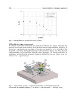
are still under control. Figure 9 shows the four combined therapeutic control agents. The
performance of robust H
∞
tracking control is estimated as
12
0
2
0
(() () () ())
0.033 0.93
( () () ()() ()())
f
f
t
TT
t
TTT
xtQxt etQetdt
wtwt ntnt rtrtdt
⎡⎤
+
⎢⎥
⎣⎦
≈≤ρ=
⎡⎤
++
⎢⎥

⎣⎦
∫
∫
E
E


Robust H
∞
Tracking Control of Stochastic Innate Immune System Under Noises

109
0 1 2 3 4 5 6 7 8 9 10 11
0
0.5
1
1.5
2
2.5
3
3.5
4
4.5
Robust H
∞
tracking control
Time unit
Concentration
x
1

Pathogens
x
2
Immune cells
x
3
Antibodies
x
4
Organ
Reference response
Take drugs

Fig. 8. The robust H
∞
tracking control of stochastic immune system under the continuous
exogenous pathogens, environmental disturbances and measurement noises. We try to
administrate a treatment after a short period (one time unit) of pathogens infection then the
stochastic immune system approach to the desired reference model quickly except for
pathogens state x
1
.

0 1 2 3 4 5 6 7 8 9 10 11
0
1
2
3
4
5

6
7
8
9
10
Control Agents
Time unit
Control concentration
u
1
u
2
u
3
u
4

Fig. 9. The robust H
∞
tracking control in the simulation example. The drug control agents
1
u
(blue, solid square line) for pathogens,
2
u for immune cells (green, solid triangle line),
3
u
for antibodies (red, solid diamond line) and
4
u for organ (magenta, solid circle line).

Obviously, the robust H
∞
tracking performance is satisfied. The conservative results are due
to the inherent conservation of solving LMI in (30)-(32).
Robust Control, Theory and Applications

110
6. Discussion and conclusion
In this study, we have developed a robust H
∞
tracking control design of stochastic immune
response for therapeutic enhancement to track a prescribed immune response under
uncertain initial states, environmental disturbances and measurement noises. Although the
mathematical model of stochastic innate immune system is taken from the literature, it still
needs to compare quantitatively with empirical evidence in practical application. For
practical implementation, accurate biodynamic models are required for treatment
application. However, model identification is not the topic of this paper. Furthermore, we
assume that not all state variables can be measured. In the measurement process, the
measured states are corrupted by noises. In this study, the statistic of disturbances,
measurement noises and initial condition are assumed unavailable and cannot be used for
the optimal stochastic tracking design. Therefore, the proposed H
∞
observer design is
employed to attenuate these measurement noises to robustly estimate the state variables for
therapeutic control and H
∞
control design is employed to attenuate disturbances to robustly
track the desired time response of stochastic immune system simultaneity. Since the
proposed H
∞

observer-based tracking control design can provide an efficient way to create a
real time therapeutic regime despite disturbances, measurement noises and initial condition
to protect suspected patients from the pathogens infection, in the future, we will focus on
applications of robust H
∞
observer-based control design to therapy and drug design
incorporating nanotechnology and metabolic engineering scheme.
Robustness is a significant property that allows for the stochastic innate immune system to
maintain its function despite exogenous pathogens, environmental disturbances, system
uncertainties and measurement noises. In general, the robust H
∞
observer-based tracking
control design for stochastic innate immune system needs to solve a complex nonlinear
Hamilton-Jacobi inequality (HJI), which is generally difficult to solve for this control design.
Based on the proposed fuzzy interpolation approach, the design of nonlinear robust H
∞

observer-based tracking control problem for stochastic innate immune system is
transformed to solve a set of equivalent linear H
∞
observer-based tracking problem. Such
transformation can then provide an easier approach by solving an LMI-constrained
optimization problem for robust H
∞
observer-based tracking control design. With the help
of the Robust Control Toolbox in Matlab instead of the HJI, we could solve these problems
for robust H
∞
observer-based tracking control of stochastic innate immune system more
efficiently. From the in silico simulation examples, the proposed robust H

∞
observer-based
tracking control of stochastic immune system could track the prescribed reference time
response robustly, which may lead to potential application in therapeutic drug design for a
desired immune response during an infection episode.
7. Appendix
7.1 Appendix A: Proof of Theorem 1
Before the proof of Theorem 1, the following lemma is necessary.
Lemma 2:
For all vectors
1
,
n
×
αβ∈R , the following inequality always holds
2
2
1
TT T T
αβ+βα≤ αα+ρββ
ρ
for any scale value 0
ρ
> .
Let us denote a Lyapunov energy function
(()) 0Vxt > . Consider the following equivalent
equation:
Robust H
∞
Tracking Control of Stochastic Innate Immune System Under Noises

111

[][]
00
(())
() () ( (0)) ( ( )) () ()
f f
tt
TT
dV x t
xtQxtdt Vx Vx xtQxt dt
dt
⎡
⎤
⎛⎞
⎡⎤
=−∞+ +
⎜⎟
⎢
⎥
⎢⎥
⎣⎦
⎝⎠
⎣
⎦
∫∫
EEEE
(A1)
By the chain rule, we get

()
(()) (()) () (())
(()) ()
() ()
TT
dVxt Vxt dxt Vxt
Fxt Dwt
dt xt dt xt
⎛⎞⎛⎞
∂∂
== +
⎜⎟⎜⎟
∂∂
⎝⎠⎝⎠
(A2)
Substituting the above equation into (A1), by the fact that
(( )) 0Vx
∞
≥ , we get

[]
()
00
(())
() () ( (0)) () () ( ()) ()
()
ff
T
tt

TT
Vxt
xtQxtdt Vx xtQxt Fxt Dwt dt
xt
⎡
⎤
⎛⎞
⎛⎞
∂
⎡⎤
⎢
⎥
⎜⎟
≤+ + +
⎜⎟
⎢⎥
⎢
⎥
⎣⎦
⎜⎟
∂
⎝⎠
⎝⎠
⎣
⎦
∫∫
EEE
(A3)
By Lemma 2, we have

2
2
(()) 1 (()) 1 (())
() () ()
() 2 () 2 ()
1 ( ()) ( ())
( ) ( )
() ()
4
TT
TT
T
TT
Vxt Vxt Vxt
Dw t Dw t w t D
xt xt xt
Vxt Vxt
DD w t w t
xt xt
⎛⎞ ⎛⎞
∂∂ ∂
=+
⎜⎟ ⎜⎟
∂∂ ∂
⎝⎠ ⎝⎠
⎛⎞
∂∂
≤+ρ
⎜⎟
∂∂

ρ
⎝⎠
(A4)
Therefore, we can obtain

[]
00
2
2
(())
() () ( (0)) () () ( ())
()
1(()) (())
( ) ( )
() ()
4
ff
T
tt
TT
T
TT
Vxt
xtQxtdt Vx xtQxt Fxt
xt
Vxt Vxt
DD w t w t dt
xt xt
⎡
⎛

⎛⎞
∂
⎡⎤
⎢
⎜
≤+ +
⎜⎟
⎢⎥
⎢
⎣⎦
⎜
∂
⎝⎠
⎝
⎣
⎤
⎞
⎛⎞
∂∂
⎟
++ρ
⎜⎟
⎟
∂∂
ρ
⎝⎠
⎠
⎦
∫∫
EEE

⎥
⎥
(A5)
By the inequality in (10), then we get

[]
2
00
() () ( (0)) () ()
ff
tt
TT
x tQxtdt Vx w twtdt
⎡
⎤⎡⎤
≤+ρ
⎢
⎥⎢⎥
⎣
⎦⎣⎦
∫∫
EEE
(A6)
If
(0) 0x = , then we get the inequality in (8).
7.2 Appendix B: Proof of Theorem 2
Let us choose a Lyapunov energy function (()) () () 0
T
Vxt x tPxt
=

> where
0
T
PP
=
>
. Then
equation (A1) is equivalent to the following:
[][]
(
)
[]
[]
00
0
11
() () ( (0)) ( ( )) () () 2 () ()
( (0)) () () 2 () (()) (()) () ()
((0)) () (
f f
f
tt
TTT
LL
t
TT
ijiji
ij
T
xtQxtdt Vx Vx xtQxt xtPxtdt

Vx x tQxt x tP h zt h zt xt Ewt dt
Vx x tQx
==
⎡⎤ ⎡ ⎤
=−∞+ +
⎢⎥ ⎢ ⎥
⎣⎦ ⎣ ⎦
⎡⎤
⎛⎞
⎛⎞
⎢⎥
⎜⎡⎤⎟
⎜⎟
≤+ + +
⎣⎦
⎜⎟
⎜⎟
⎢⎥
⎝⎠
⎝⎠
⎣⎦
=+
∫∫
∑∑
∫
EEEE
EE A
EE

0

11
) (()) (()) 2 () () 2 () ()
f
LL
t
TT
ij ij i
ij
thzthztxtPxtxtPEwtdt
==
⎡
⎤
⎛⎞
⎡⎤
⎢
⎥
⎜⎟
++
⎣⎦
⎜⎟
⎢
⎥
⎝⎠
⎣
⎦
∑∑
∫
A
(A7)
Robust Control, Theory and Applications

112
By Lemma 2, we have

2() () () () () ()
TT TT
iii
xtPEwt xtPEwt wtEPxt=+
2
2
1
() () () ()
TT T
ii
xtPEEPxt wtwt≤+ρ
ρ
(A8)
Therefore, we can obtain
[]
(
00
11
2
2
() () ( (0)) () () (()) (()) ( )
1
( ) ( ) ( ) ( )

ff
LL

tt
TTTT
ij ijij
ij
TT T
ii
xtQxtdt Vx xtQxt hzt hzt xP Px
xtPEEPxt wtwtdt
==
⎡⎤ ⎡
⎡
≤
++ ++
⎣
⎢⎥ ⎢
⎣⎦ ⎣
⎤
⎞
⎤
++ρ=
⎥
⎟
⎥
⎟
ρ
⎥
⎦
⎠
⎦
∑∑

∫∫
EEE AA
[]
0
11
2
2
( (0)) ( ) ( ) ( ( )) ( ( )) ( )
1
+ ( ) ( ) ( )
f
LL
t
TTT
i j ij ij
ij
TT
ii
Vx x tQxt h zt h zt x t P P
PE E P x t w t w t dt
==
⎡
⎛
⎡
⎢
⎜
=
++ ++
⎣
⎜

⎢
⎝
⎣
⎤
⎞
⎤
+ρ
⎥
⎟
⎥
⎟
ρ
⎥
⎦
⎠
⎦
∑∑
∫
EE AA
(A9)
By the inequality in (20), then we get

[]
2
00
() () ( (0)) () ()
ff
tt
TT
xtQxtdt Vx wtwtdt

⎡
⎤⎡⎤
≤+ρ
⎢
⎥⎢⎥
⎣
⎦⎣⎦
∫∫
EEE
(A10)
This is the inequality in (9). If
(0) 0x
=
, then we get the inequality in (8).
7.3 Appendix C: Proof of Lemma 1
For
[
]
123456
0eeeeee
≠
, if (25)-(26) hold, then
111 1415 1112
22223 21222324
33233 363233
441 44
551 55 42 44
66366
00 0 0000
0 000 0 0

0000000
00 00 000000
000 0 0 00 0
00 00 000000
T
ea aa bb
eaa bbbb
eaa abb
ea a
ea a b b
eaa
⎧
⎡⎤ ⎡ ⎤⎡ ⎤
⎪
⎢⎥ ⎢ ⎥⎢ ⎥
⎪
⎢⎥ ⎢ ⎥⎢ ⎥
⎪
⎢⎥ ⎢ ⎥⎢ ⎥
⎪
+
⎢⎥ ⎢ ⎥⎢ ⎥
⎨
⎢⎥ ⎢ ⎥⎢ ⎥
⎢⎥ ⎢ ⎥⎢ ⎥
⎢⎥ ⎢ ⎥⎢ ⎥
⎢⎥ ⎢ ⎥⎢ ⎥
⎣⎦ ⎣ ⎦⎣ ⎦
1
2

3
4
5
6
e
e
e
e
e
e
⎫
⎡
⎤
⎪
⎢
⎥
⎪
⎢
⎥
⎪
⎢
⎥
⎪
⎢
⎥
⎬
⎢
⎥
⎪⎪
⎢

⎥
⎪⎪
⎢
⎥
⎪⎪
⎢
⎥
⎪⎪
⎣
⎦
⎩⎭

111 1415 1
22223 211112
33233 363221222324
441 44 4 3 3233
551 55 5 5
663666
00 0
0 000 00
000
00 00 0 0
000 0
00 00
T
T
ea aa e
eaa eebb
eaa aeebbbb
ea a e e bb

ea a e e
eaae
⎡⎤⎡ ⎤⎡⎤
⎢⎥⎢ ⎥⎢⎥
⎡⎤
⎢⎥⎢ ⎥⎢⎥
⎢⎥
⎢⎥⎢ ⎥⎢⎥
⎢⎥
=+
⎢⎥⎢ ⎥⎢⎥
⎢⎥
⎢⎥⎢ ⎥⎢⎥
⎢⎥
⎢⎥⎢ ⎥⎢⎥
⎣⎦
⎢⎥⎢ ⎥⎢⎥
⎢⎥⎢ ⎥⎢⎥
⎣⎦⎣ ⎦⎣⎦
1
2
3
42 44 5
0
00
e
e
e
bbe
⎡⎤⎡⎤

⎢⎥⎢⎥
⎢⎥⎢⎥
<
⎢⎥⎢⎥
⎢⎥⎢⎥
⎣⎦⎣⎦


This implies that (27) holds. Therefore, the proof is completed.
Robust H
∞
Tracking Control of Stochastic Innate Immune System Under Noises

113
7.4 Appendix D: Parameters of the Fuzzy System, control gains and observer gains
The nonlinear innate immune system in (33) could be approximated by a Takagi-Sugeno
Fuzzy system. By the fuzzy modeling method (Takagi & Sugeno, 1985), the matrices of the
local linear system
i
A , the parameters B , C , D ,
j
K
and
i
L are calculated as follows:
1
0000
3100
0.5 1 1.5 0
0.5 0 0 1

⎡⎤
⎢⎥
−
⎢⎥
=
⎢⎥
−−
⎢⎥
−
⎣⎦
A
,
2
0000
3100
0.5 1 1.5 0
0.5 0 0 1
⎡
⎤
⎢
⎥
−
⎢
⎥
=
⎢
⎥
−−
⎢
⎥

−
⎣
⎦
A
,
3
0000
3100
0.5 1 1.5 0
0.5 0 0 1
⎡
⎤
⎢
⎥
−
⎢
⎥
=
⎢
⎥
−−
⎢
⎥
−
⎣
⎦
A
,
4
2000

9100
1.5 1 1.5 0
0.5 0 0 1
−
⎡⎤
⎢⎥
−
⎢⎥
=
⎢⎥
−−
⎢⎥
−
⎣⎦
A ,
5
2000
9100
1.5 1 1.5 0
0.5 0 0 1
−
⎡
⎤
⎢
⎥
−−
⎢
⎥
=
⎢

⎥
−−
⎢
⎥
−
⎣
⎦
A ,
6
20 0 0
9100
1.5 1 1.5 0
0.5 0 0 1
−
⎡
⎤
⎢
⎥
−
⎢
⎥
=
⎢
⎥
−−
⎢
⎥
−
⎣
⎦

A ,
7
4000
15 1 0 0
2.5 1 1.5 0
0.5 0 0 1
−
⎡⎤
⎢⎥
−
⎢⎥
=
⎢⎥
−−
⎢⎥
−
⎣⎦
A ,
8
40 0 0
15 1 0 0
2.5 1 1.5 0
0.5 0 0 1
−
⎡
⎤
⎢
⎥
−−
⎢

⎥
=
⎢
⎥
−−
⎢
⎥
−
⎣
⎦
A ,
9
4000
15 1 0 0
2.5 1 1.5 0
0.5 0 0 1
−
⎡
⎤
⎢
⎥
−
⎢
⎥
=
⎢
⎥
−−
⎢
⎥

−
⎣
⎦
A
1000
0100
0010
0001
−
⎡
⎤
⎢
⎥
−
⎢
⎥
=
⎢
⎥
⎢
⎥
−
⎣
⎦
B
,
0100
0010
0001
C

⎡
⎤
⎢
⎥
=
⎢
⎥
⎢
⎥
⎣
⎦
,
1000
0100
0010
0001
D
⎡
⎤
⎢
⎥
⎢
⎥
=
⎢
⎥
⎢
⎥
⎣
⎦

17.712 0.14477 -0.43397 0.18604
0.20163 18.201 0.37171 -0.00052926
0.51947 -0.31484 -13.967 -0.052906
0.28847 0.0085838 0.046538 14.392
j
K
⎡
⎤
⎢
⎥
⎢
⎥
=
⎢
⎥
⎢
⎥
⎣
⎦
, 1, ,9j = 
12.207 -26.065 22.367
93.156 -8.3701 7.8721
-8.3713 20.912 -16.006
7.8708 -16.005 14.335
i
L
⎡
⎤
⎢

⎥
⎢
⎥
=
⎢
⎥
⎢
⎥
⎣
⎦
,
1, ,9
i
=

.
8. References
Asachenkov, A.L. (1994) Disease dynamics. Birkhäuser Boston.
Balas, G., Chiang, R., Packard, A. & Safonov, M. (2007)
MATLAB: Robust Control Toolbox 3
User's Guide
. The MathWorks, Inc.
Bell, D.J. & Katusiime, F. (1980) A Time-Optimal Drug Displacement Problem,
Optimal
Control Applications & Methods
, 1, 217-225.
Robust Control, Theory and Applications

114
Bellman, R. (1983) Mathematical methods in medicine. World Scientific, Singapore.

Bonhoeffer, S., May, R.M., Shaw, G.M. & Nowak, M.A. (1997) Virus dynamics and drug
therapy,
Proc. Natl. Acad. Sci. USA, 94, 6971-6976.
Boyd, S.P. (1994)
Linear matrix inequalities in system and control theory. Society for Industrial
and Applied Mathematics, Philadelphia.
Carson, E.R., Cramp, D.G., Finkelstein, F. & Ingram, D. (1985) Control system concepts and
approaches in clinical medicine. In Carson, E.R. & Cramp, D.G. (eds),
Computers and
Control in Clinical Medicine
. Plenum Press, New York, 1-26.
Chen, B.S., Chang, C.H. & Chuang, Y.J. (2008) Robust model matching control of immune
systems under environmental disturbances: dynamic game approach,
J Theor Biol,
253, 824-837.
Chen, B.S., Tseng, C.S. & Uang, H.J. (1999) Robustness design of nonlinear dynamic systems
via fuzzy linear control,
IEEE Transactions on Fuzzy Systems, 7, 571-585.
Chen, B.S., Tseng, C.S. & Uang, H.J. (2000) Mixed H-2/H-infinity fuzzy output feedback
control design for nonlinear dynamic systems: An LMI approach,
IEEE Transactions
on Fuzzy Systems
, 8, 249-265.
Chizeck, H.J. & Katona, P.G. (1985) Closed-loop control. In Carson, E.R. & Cramp, D.G.
(eds),
Computers and Control in Clinical Medicine. Plenum Press, New York, 95-151.
De Boer, R.J. & Boucher, C.A. (1996) Anti-CD4 therapy for AIDS suggested by mathematical
models,
Proc. Biol. Sci. , 263, 899-905.
Gentilini, A., Morari, M., Bieniok, C., Wymann, R. & Schnider, T.W. (2001) Closed-loop

control of analgesia in humans.
Proc. IEEE Conf. Decision and Control. Orlando, 861-
866.
Janeway, C. (2005)
Immunobiology : the immune system in health and disease. Garland, New
York.
Jang, J S.R., Sun, C T. & Mizutani, E. (1997)
Neuro-fuzzy and soft computing : a computational
approach to learning and machine intelligence
. Prentice Hall, Upper Saddle River, NJ.
Jelliffe, R.W. (1986) Clinical applications of pharmacokinetics and control theory: planning,
monitoring, and adjusting regimens of aminoglycosides, lidocaine, digitoxin, and
digoxin. In Maronde, R.F. (ed),
Topics in clinical pharmacology and therapeutics.
Springer, New York, 26-82.
Kim, E., Park, M. & Ji, S.W. (1997) A new approach to fuzzy modeling,
IEEE Transactions on
Fuzzy Systems
, 5, 328-337.
Kirschner, D., Lenhart, S. & Serbin, S. (1997) Optimal control of the chemotherapy of HIV,
J.
Math. Biol.
, 35, 775-792.
Kwong, G.K., Kwok, K.E., Finegan, B.A. & Shah, S.L. (1995) Clinical evaluation of long range
adaptive control for meanarterial blood pressure regulation.
Proc. Am. Control Conf.,
Seattle, 786-790.
Li, T.H.S., Chang, S.J. & Tong, W. (2004) Fuzzy target tracking control of autonomous
mobile robots by using infrared sensors,
IEEE Transactions on Fuzzy Systems, 12,

491-501.
Lian, K.Y., Chiu, C.S., Chiang, T.S. & Liu, P. (2001) LMI-based fuzzy chaotic synchronization
and communications,
IEEE Transactions on Fuzzy Systems, 9, 539-553.
Lydyard, P.M., Whelan, A. & Fanger, M.W. (2000)
Instant notes in immunology. Springer,
New York.
Robust H
∞
Tracking Control of Stochastic Innate Immune System Under Noises

115
Ma, X.J., Sun, Z.Q. & He, Y.Y. (1998) Analysis and design of fuzzy controller and fuzzy
observer,
IEEE Transactions on Fuzzy Systems, 6, 41-51.
Marchuk, G.I. (1983)
Mathematical models in immunology. Optimization Software, Inc.
Worldwide distribution rights by Springer, New York.
Milutinovic, D. & De Boer, R.J. (2007) Process noise: an explanation for the fluctuations in
the immune response during acute viral infection,
Biophys J, 92, 3358-3367.
Nowak, M.A. & May, R.M. (2000)
Virus dynamics : mathematical principles of immunology and
virology
. Oxford University Press, Oxford.
Nowak, M.A., May, R.M., Phillips, R.E., Rowland-Jones, S., Lalloo, D.G., McAdam, S.,
Klenerman, P., Koppe, B., Sigmund, K., Bangham, C.R. & et al. (1995) Antigenic
oscillations and shifting immunodominance in HIV-1 infections,
Nature, 375, 606-
611.

Parker, R.S., Doyle, J.F., III., Harting, J.E. & Peppas, N.A. (1996) Model predictive control for
infusion pump insulin delivery.
Proceedings of the 18th Annual International
Conference of the IEEE Engineering in Medicine and Biology Society
. Amsterdam, 1822-
1823.
Perelson, A.S., Kirschner, D.E. & De Boer, R. (1993) Dynamics of HIV infection of CD4+ T
cells,
Math. Biosci., 114, 81-125.
Perelson, A.S., Neumann, A.U., Markowitz, M., Leonard, J.M. & Ho, D.D. (1996) HIV-1
dynamics in vivo: virion clearance rate, infected cell life-span, and viral generation
time,
Science, 271, 1582-1586.
Perelson, A.S. & Weisbuch, G. (1997) Immunology for physicists,
Reviews of Modern Physics,
69, 1219-1267.
Piston, D.W. (1999) Imaging living cells and tissues by two-photon excitation microscopy,
Trends Cell Biol, 9, 66-69.
Polycarpou, M.M. & Conway, J.Y. (1995) Modeling and control of drug delivery systems
using adaptive neuralcontrol methods.
Proc. Am. Control Conf., Seattle, 781-785.
Robinson, D.C. (1986) Topics in clinical pharmacology and therapeutics. In Maronde, R.F.
(ed),
Principles of Pharmacokinetics. Springer, New York, 1-12.
Rundell, A., HogenEsch, H. & DeCarlo, R. (1995) Enhanced modeling of the immune system
to incorporate naturalkiller cells and memory.
Proc. Am. Control Conf., Seattle, 255-
259.
Schumitzky, A. (1986) Stochastic control of pharmacokinetic systems. In Maronde, R.F. (ed),
Topics in clinical pharmacology and therapeutics. Springer, New York, 13-25.

Stafford, M.A., Corey, L., Cao, Y., Daar, E.S., Ho, D.D. & Perelson, A.S. (2000) Modeling
plasma virus concentration during primary HIV infection,
J. Theor. Biol., 203, 285-
301.
Stengel, R.F., Ghigliazza, R., Kulkarni, N. & Laplace, O. (2002a) Optimal control of innate
immune response,
Optimal Control Applications & Methods, 23, 91-104.
Stengel, R.F., Ghigliazza, R.M. & Kulkarni, N.V. (2002b) Optimal enhancement of immune
response,
Bioinformatics, 18, 1227-1235.
Sugeno, M. & Kang, G.T. (1988) Structure identification of fuzzy model,
Fuzzy Sets and
Systems
, 28, 15-33.
Swan, G.W. (1981) Optimal-Control Applications in Biomedical-Engineering - a Survey,
Optimal Control Applications & Methods, 2, 311-334.
Robust Control, Theory and Applications

116
Takagi, T. & Sugeno, M. (1985) Fuzzy Identification of Systems and Its Applications to
Modeling and Control,
IEEE Transactions on Systems Man and Cybernetics, 15, 116-
132.
Tanaka, K., Ikeda, T. & Wang, H.O. (1998) Fuzzy regulators and fuzzy observers: Relaxed
stability conditions and LMI-based designs,
IEEE Transactions on Fuzzy Systems, 6,
250-265.
Tseng, C.S. (2008) A novel approach to H-infinity decentralized fuzzy-observer-based fuzzy
control design for nonlinear interconnected systems,
IEEE Transactions on Fuzzy

Systems
, 16, 1337-1350.
van Rossum, J.M., Steyger, O., van Uem, T., Binkhorst, G.J. & Maes, R.A.A. (1986)
Pharmacokinetics by using mathematical systems dynamics. In Eisenfeld, J. &
Witten, M. (eds),
Modelling of biomedical systems. Elsevier, Amsterdam, 121-126.
Wang, H.O., Tanaka, K. & Griffin, M.F. (1996) An approach to fuzzy control of nonlinear
systems: Stability and design issues,
IEEE Transactions on Fuzzy Systems, 4, 14-23.
Wein, L.M., D'Amato, R.M. & Perelson, A.S. (1998) Mathematical analysis of antiretroviral
therapy aimed at HIV-1 eradication or maintenance of low viral loads,
J. Theor.
Biol.
, 192, 81-98.
Wiener, N. (1948)
Cybernetics; or, Control and communication in the animal and the machine.
Technology Press, Cambridge.
Wodarz, D. & Nowak, M.A. (1999) Specific therapy regimes could lead to long-term
immunological control of HIV,
Proc. Natl. Acad. Sci. USA, 96, 14464-14469.
Wodarz, D. & Nowak, M.A. (2000) CD8 memory, immunodominance, and antigenic escape,
Eur. J. Immunol., 30, 2704-2712.
Zhou, K., Doyle, J.C. & Glover, K. (1996)
Robust and optimal control. Prentice Hall, Upper
Saddle River, N.J.

6
Robust H
∞
Reliable Control of

Uncertain Switched Nonlinear
Systems with Time-varying Delay
Ronghao Wang
1
, Jianchun Xing
1
,
Ping Wang
1
, Qiliang Yang
1
and Zhengrong Xiang
2

1
PLA University of Science and Technology
2
Nanjing University of Science and Technology
China
1. Introduction
Switched systems are a class of hybrid system consisting of subsystems and a switching law,
which define a specific subsystem being activated during a certain interval of time. Many
real-world processes and systems can be modeled as switched systems, such as the
automobile direction-reverse systems, computer disk systems, multiple work points control
systems of airplane and so on. Therefore, the switched systems have the wide project
background and can be widely applied in many domains (Wang, W. & Brockett, R. W., 1997;
Tomlin, C. et al., 1998; Varaiya, P., 1993). Besides switching properties, when modeling a
engineering system, system uncertainties that occur as a result of using approximate system
model for simplicity, data errors for evaluation, changes in environment conditions, etc, also
exit naturally in control systems. Therefore, both of switching and uncertainties should be

integrated into system model. Recently, study of switched systems mainly focuses on
stability and stabilization (Sun, Z. D. & Ge, S. S., 2005; Song, Y. et al., 2008; Zhang, Y. et al.,
2007). Based on linear matrix inequality technology, the problem of robust control for the
system is investigated in the literature (Pettersson, S. & Lennartson, B., 2002). In order to
guarantee H
∞
performance of the system, the robust H
∞
control is studied using linear matrix
inequality method in the literature (Sun, W. A. & Zhao, J., 2005).
In many engineering systems, the actuators may be subjected to faults in special
environment due to the decline in the component quality or the breakage of working
condition which always leads to undesirable performance, even makes system out of
control. Therefore, it is of interest to design a control system which can tolerate faults of
actuators. In addition, many engineering systems always involve time delay phenomenon,
for instance, long-distance transportation systems, hydraulic pressure systems, network
control systems and so on. Time delay is frequently a source of instability of feedback
systems. Owing to all of these, we shouldn’t neglect the influence of time delay and
probable actuators faults when designing a practical control system. Up to now, research
activities of this field for switched system have been of great interest. Stability analysis of a
class of linear switching systems with time delay is presented in the literature (Kim, S. et al.,
2006). Robust H
∞
control for discrete switched systems with time-varying delay is discussed
Robust Control, Theory and Applications

118
in the literature (Song, Z. Y. et al., 2007). Reliable guaranteed-cost control for a class of
uncertain switched linear systems with time delay is investigated in the literature (Wang, R.
et al., 2006). Considering that the nonlinear disturbance could not be avoided in several

applications, robust reliable control for uncertain switched nonlinear systems with time
delay is studied in the literature (Xiang, Z. R. & Wang, R. H., 2008). Furthermore, Xiang and
Wang (Xiang, Z. R. & Wang, R. H., 2009) investigated robust L
∞
reliable control for uncertain
nonlinear switched systems with time delay.
Above the problems of robust reliable control for uncertain nonlinear switched time delay
systems, the time delay is treated as a constant. However, in actual operation, the time delay
is usually variable as time. Obviously, the system model couldn’t be described appropriately
using constant time delay in this case. So the paper focuses on the system with time-varying
delay. Besides, it is considered that H
∞
performance is always an important index in control
system. Therefore, in order to overcome the passive effect of time-varying delay for
switched systems and make systems be anti-jamming and fault-tolerant, this paper
addresses the robust H
∞
reliable control for nonlinear switched time-varying delay systems
subjected to uncertainties. The multiple Lyapunov-Krasovskii functional method is used to
design the control law. Compared with the multiple Lyapunov function adopted in the
literature (Xiang, Z. R. & Wang, R. H., 2008; Xiang, Z. R. & Wang, R. H., 2009), the multiple
Lyapunov-Krasovskii functional method has less conservation because the more system
state information is contained in the functional. Moreover, the controller parameters can be
easily obtained using the constructed functional.
The organization of this paper is as follows. At first, the concept of robust reliable controller,
γ
-suboptimal robust H
∞
reliable controller and
γ

-optimal robust H
∞
reliable controller are
presented. Secondly, fault model of actuator for system is put forward. Multiple Lyapunov-
Krasovskii functional method and linear matrix inequality technique are adopted to design
robust H
∞
reliable controller. Meanwhile, the corresponding switching law is proposed to
guarantee the stability of the system. By using the key technical lemma, the design problems
of
γ
-suboptimal robust H
∞
reliable controller and
γ
-optimal robust H
∞
reliable controller
can be transformed to the problem of solving a set of the matrix inequalities. It is worth to
point that the matrix inequalities in the
γ
-optimal problem are not linear, then we make use
of variable substitute method to acquire the controller gain matrices and
γ
-optimal problem
can be transferred to solve the minimal upper bound of the scalar
γ
. Furthermore, the
iteration solving process of optimal disturbance attenuation performance
γ

is presented.
Finally, a numerical example shows the effectiveness of the proposed method. The result
illustrates that the designed controller can stabilize the original system and make it be of H
∞

disturbance attenuation performance when the system has uncertain parameters and
actuator faults.
Notation Throughout this paper,
T
A denotes transpose of matrix A ,
2
[0, )L ∞ denotes
space of square integrable functions on
[0, )
∞
. ()xt denotes the Euclidean norm. I is an
identity matrix with appropriate dimension.
{}
i
diag a denotes diagonal matrix with the
diagonal elements
i
a , 1,2, ,iq
=
 . 0S
<
(or 0S > ) denotes S is a negative (or positive)
definite symmetric matrix. The set of positive integers is represented by Z
+
. AB≤ (or

AB≥ ) denotes AB
−
is a negative (or positive) semi-definite symmetric matrix. ∗ in
AB
C
⎡⎤
⎢⎥
∗
⎣⎦
represents the symmetric form of matrix, i.e.
T
B∗= .
Robust H
∞
Reliable Control of Uncertain Switched Nonlinear Systems with Time-varying Delay

119
2. Problem formulation and preliminaries
Consider the following uncertain switched nonlinear system with time-varying delay

() () () () ()
ˆˆ
ˆ
() () ( ()) () () ((),)
f
tdt t t t
xt A xt A xt dt B u t D wt f xt t
σσ σ σσ
=+−+ + +


(1)

() () ()
() () () ()
f
tt t
zt C xt G u t N wt
σσ σ
=+ +
(2)

() (), [ ,0]xt t t
φ
ρ
=
∈− (3)
where ( )
m
xt R∈ is the state vector, ( )
q
wt R∈ is the measurement noise, which belongs to
2
[0, )L ∞ , ( )
p
zt R∈ is the output to be regulated, ( )
f
l
ut R
∈
is the control input of actuator

fault. The function
():[0, ) {1,2, , }tNN
σ
∞→ =  is switching signal which is deterministic,
piecewise constant, and right continuous, i.e.
11
( ) :{(0, (0)),( , ( )), ,( , ( ))},
kk
tttttkZ
σσ σ σ
+
∈ ,
where
k
t denotes the k th switching instant. Moreover, ()ti
σ
=
means that the i th
subsystem is activated,
N is the number of subsystems. ()t
φ
is a continuous vector-valued
initial function. The function
()dt denotes the time-varying state delay satisfying
0() ,() 1
dt dt
ρμ
≤≤<∞ ≤<

for constants

ρ
,
μ
, and (,):
i
f ii
mm
RRR×→
for iN∈ are
unknown nonlinear functions satisfying

((),) ()
ii
f
xt t Uxt≤ (4)
where
i
U are known real constant matrices.
The matrices
ˆ
i
A ,
ˆ
di
A and
ˆ
i
B for iN
∈
are uncertain real-valued matrices of appropriate

dimensions. The matrices
ˆ
i
A ,
ˆ
di
A and
ˆ
i
B can be assumed to have the form

12
ˆˆ
ˆ
[, ,][, ,] ()[ , , ]
i dii i dii ii idi i
A
AB AAB HFtEEE=+
(5)
where
1
,,,,,
idii i idi
AA BHE E and
2i
E for iN
∈
are known real constant matrices with proper
dimensions,
1

,,
iidi
HE E and
2i
E denote the structure of the uncertainties, and ()
i
Ft are
unknown time-varying matrices that satisfy

() ()
T
ii
FtFt I
≤
(6)
The parameter uncertainty structure in equation (5) has been widely used and can represent
parameter uncertainty in many physical cases (Xiang, Z. R. & Wang, R. H., 2009; Cao, Y. et
al., 1998).
In actual control system, there inevitably occurs fault in the operation process of actuators.
Therefore, the input control signal of actuator fault is abnormal. We use
()ut and
()
f
ut
to
represent the normal control input and the abnormal control input, respectively. Thus, the
control input of actuator fault can be described as
() ()
f
i

ut Mut= (7)
where
i
M
is the actuator fault matrix of the form

12
{,,,}
iiiil
M
diag m m m
=
 , 0
ik ik ik
mmm
≤
≤≤, 1
ik
m ≥ ,
1,2, ,kl
=

(8)
Robust Control, Theory and Applications

120
For simplicity, we introduce the following notation

012
{,,,}

iiiil
M
diag m m m
=
 

(9)

12
{,,,}
iiiil
Jdiagjj j=  (10)

12
{,,,}
iiiil
Ldiagll l
=
 (11)
where
1
()
2
ik ik ik
mmm=+

,
ik ik
ik
ik ik

mm
j
mm
−
=
+
,
ik ik
ik
ik
mm
l
m
−
=



By equation (9)-(11), we have

0
()
ii i
M
MIL
=
+ ,
ii
LJI
≤

≤ (12)
where
i
L represents the absolute value of diagonal elements in matrix
i
L , i.e.

12
{,,,}
iiiil
Ldia
g
ll l= 

Remark 1
1
ik
m =
means normal operation of the k th actuator control signal of the i th
subsystem. When
0
ik
m
=
, it covers the case of the complete fault of the k th actuator control
signal of the
i th subsystem. When 0
ik
m > and 1
ik

m
≠
, it corresponds to the case of partial
fault of the
k th actuator control signal of the i th subsystem.
Now, we give the definition of robust
H
∞
reliable controller for the uncertain switched
nonlinear systems with time-varying delay.
Definition 1 Consider system (1) with
() 0wt
≡
. If there exists the state feedback controller
()
() ()
t
ut K xt
σ
= such that the closed loop system is asymptotically stable for admissible
parameter uncertainties and actuator fault under the switching law
()t
σ
,
()
() ()
t
ut K xt
σ
= is

said to be a robust reliable controller.
Definition 2 Consider system (1)-(3). Let 0
γ
> be a positive constant, if there exists the
state feedback controller
()
() ()
t
ut K xt
σ
=
and the switching law ()t
σ
such that
i.
With
() 0wt ≡
, the closed system is asymptotically stable.
ii.
Under zero initial conditions, i.e. () 0xt
=
([,0])t
ρ
∈
− , the following inequality holds

22
() ()zt wt
γ
≤

,
2
() [0, )wt L
∀
∈∞, () 0wt
≠
(13)
()
() ()
t
ut K xt
σ
= is said to be
γ
-suboptimal robust H
∞
reliable controller with disturbance
attenuation performance
γ
. If there exists a minimal value of disturbance attenuation
performance
γ
,
()
() ()
t
ut K xt
σ
=
is said to be

γ
-optimal robust H
∞
reliable controller.
The following lemmas will be used to design robust
H
∞
reliable controller for the uncertain
switched nonlinear system with time-varying delay.
Lemma 1 (Boyd, S. P. et al., 1994; Schur complement) For a given matrix
11 12
21 22
SS
S
SS
⎡
⎤
=
⎢
⎥
⎣
⎦

with
11 11
T
SS= ,
22 22
T
SS= ,

12 21
T
SS= , then the following conditions are equivalent
i 0
S <
ii
11
0S < ,
1
22 21 11 12
0SSSS
−
−
<
iii
22
0S <
,
1
11 12 22 21
0SSSS
−
−
<
Robust H
∞
Reliable Control of Uncertain Switched Nonlinear Systems with Time-varying Delay

121
Lemma 2

(Cong, S. et al., 2007) For matrices X and Y of appropriate dimension and 0Q > ,
we have
1TT T T
XY YX XQX YQ Y
−
+≤ +

Lemma 3 (Lien, C.H., 2007) Let
,,
YDE
and F be real matrices of appropriate dimensions
with
F satisfying
T
FF
=
, then for all
T
FF I
≤


0
TT T
YDFEEFD
+
+<

if and only if there exists a scalar 0
ε

> such that
1
0
TT
YDD EE
εε
−
+
+<

Lemma 4 (Xiang, Z. R. & Wang, R. H., 2008) For matrices
12
,RR, the following inequality
holds
1
122 111 22
() ()
TT T T
RtRR tR RUR RUR
Τ
ΣΣββ
−
+≤+

where 0
β
> , ()t
Σ
is time-varying diagonal matrix, U is known real constant matrix
satisfying

()tU
Σ
≤ , ()t
Σ
represents the absolute value of diagonal elements in matrix
()t
Σ
.
Lemma 5 (Peleties, P. & DeCarlo, R. A., 1991) Consider the following system

()
() (())
t
xt
f
xt
σ
=

(14)

where
():[0, ) {1,2, , }tNN
σ
∞→ = 
. If there exist a set of functions :,
m
i
VR Ri N→ ∈ such
that

(i)
i
V
is a positive definite function, decreasing and radially unbounded;
(ii)
(()) ( ) () 0
iii
dV x t dt V x f x
=
∂∂ ≤
is negative definite along the solution of (14);
(iii) ( ( )) ( ( ))
j
kik
Vxt Vxt≤ when the i th subsystem is switched to the
j
th subsystem
,,ij N∈

ij≠
at the switching instant ,
k
tkZ
+
=

, then system (14) is asymptotically stable.
3. Main results
3.1 Condition of stability
Consider the following unperturbed switched nonlinear system with time-varying delay

() () ()
() () ( ()) ((),)
tdt t
xt A xt A xt dt
f
xt t
σσ σ
=
+−+

(15)

() (), [ ,0]xt t t
φ
ρ
=
∈− (16)

The following theorem presents a sufficient condition of stability for system (15)-(16).
Theorem 1 For system (15)-(16), if there exists symmetric positive definite matrices ,
i
PQ,
and the positive scalar
δ
such that


i
PI

δ
<
(17)
Robust Control, Theory and Applications

122

0
*(1)
TT
ii ii j i i idi
A P PA P Q U U PA
Q
δ
μ
⎡⎤
++++
<
⎢⎥
−−
⎢⎥
⎣
⎦
(18)
where
,,ijijN≠ ∈ , then systems (15)-(16) is asymptotically stable under the switching law
() ar
g
min{ () ()}
T

i
iN
txtPxt
σ
∈
=
.
Proof For the i th subsystem, we define Lyapunov-Krasovskii functional
()
(()) () () () ()
t
TT
ii
tdt
Vxt x tPxt x Qx d
τ
ττ
−
=+
∫

where
,
i
PQ are symmetric positive definite matrices. Along the trajectories of system (15),
the time derivative of
()
i
Vt is given by
(()) () () () () () () (1 ()) ( ()) ( ())

() () () () () () (1 ) ( ()) ( ())
2 ( ) [ ( ) ( ( )) ( ( ), )] ( ) ( )
TTT T
iii
TTT T
ii
TT
ii di i
V xt x tPxt x tPxt x tQxt dt x t dt Qxt dt
x tPxt x tPxt x tQxt x t dt Qxt dt
x tP Axt A xt dt f xt t x tQxt
μ
=++−−−−
≤++−−−−
=+−++





(1 ) ( ()) ( ())
()( )() 2 () ( ()) 2 () ( (),)
(1 ) ( ()) ( ())
T
TT T T
ii ii idi ii
T
xtdtQxtdt
x t AP PA Qxt x tPA xt dt x tP
f

xt t
xtdtQxtdt
μ
μ
−− − −
=+++ −+
−− − −



From Lemma 2, it is established that

2 () ( (),) () () ((),) ((),)
TTT
ii i i ii
xtP
f
xt t x tPxt
f
xt tP
f
xt t≤+

From expressions (4) and (17), it follows that
2 () ( (),) () () ( (),) ((),) ()( )()
TTT TT
ii i i i i i i
xtP
f
xt t x tPxt

f
xt t
f
xt t x t P U U xt
δδ
≤+ ≤+
Therefore, we can obtain that
(()) ()( )() 2 () ( ())
(1 ) ( ()) ( ())
TT T T
iiiiiiiiidi
T
T
i
Vxt x t AP PA Q P UUxt x tPAxt dt
xtdtQxtdt
δ
μ
ηΘη
≤++++ + −
− − − −
=


where
()
,
(())
*(1)
TT

ii ii i i i idi
i
xt
AP PA Q P UU PA
xt dt
Q
δ
ηΘ
μ
⎡
⎤
⎡⎤
++++
= =
⎢
⎥
⎢⎥
−
−−
⎢
⎥
⎣⎦
⎣
⎦

From (18), we have
{,0}0
iji
diag P P
Θ

+
−< (19)
Using
T
η
and
η
to pre- and post- multiply the left-hand term of expression (19) yields
(()) ()( )()
T
iij
Vxt x t P Pxt<−

(20)
Robust H
∞
Reliable Control of Uncertain Switched Nonlinear Systems with Time-varying Delay

123
The switching law () ar
g
min{ () ()}
T
i
iN
txtPxt
σ
∈
= expresses that for ,,ij Ni j
∈

≠ , there holds the
inequality

() () () ()
TT
ij
xtPxt xtPxt≤
(21)
(20) and (21) lead to

(()) 0
i
Vxt
<

(22)
Obviously, the switching law
() ar
g
min{ () ()}
T
i
iN
txtPxt
σ
∈
=
also guarantees that Lyapunov-
Krasovskii functional value of the activated subsystem is minimum at the switching instant.
From Lemma 5, we can obtain that system (15)-(16) is asymptotically stable. The proof is

completed.
■
Remark 2 It is worth to point that the condition (21) doesn’t imply
i
j
PP
≤
, for the state ()xt
doesn’t represent all the state in domain
m
R but only the state of the i th activated subsystem.
3.2 Design of robust reliable controller
Consider system (1) with () 0wt
≡


() () () ()
ˆˆ
ˆ
() () ( ()) () ( (),)
f
tdt t t
xt A xt A xt dt B u t f xt t
σσ σσ
=+−+ +

(23)

() (), [ ,0]xt t t
φ

ρ
=
∈− (24)
By (7), for the i th subsystem the feedback control law can be designed as

() ()
f
ii
ut MKxt=
(25)
Substituting (25) to (23), the corresponding closed-loop system can be written as

ˆ
() () ( ()) ( (),)
idi i
xt Axt A xt dt
f
xt t=+−+


(26)
where
ˆ
ˆ
iiiii
A
ABMK=+

, iN
∈

.
The following theorem presents a sufficient existing condition of the robust reliable
controller for system (23)-(24).
Theorem 2 For system (23)-(24), if there exists symmetric positive definite matrices ,
i
XS,
matrix
i
Y and the positive scalar
λ
such that

i
XI
λ
>
(27)

*(1)0 00 0
** 0000
0
*** 000
**** 00
***** 0
******
TT
idi iiiiii
T
di
j

AS H X X XU
SSE
I
I
S
X
I
ΨΦ
μ
λ
⎡⎤
⎢⎥
−−
⎢⎥
⎢⎥
−
⎢⎥
⎢⎥
<
−
⎢⎥
−
⎢⎥
⎢⎥
−
⎢⎥
⎢⎥
−
⎣⎦
(28)

Robust Control, Theory and Applications

124
where ,,ijijN≠ ∈ , ( )
T
iiiiii iiiii
A
XBMY AXBMY
Ψ
=+ + + ,
12iiiiii
EX EMY
Φ
=
+ , then there
exists the robust reliable state feedback controller

()
() ()
t
ut K xt
σ
=
,
1
iii
KYX
−
= (29)
and the switching law is designed as

1
() ar
g
min{ () ()}
T
i
iN
txtXxt
σ
−
∈
= , the closed-loop system is
asymptotically stable.
Proof From (5) and Theorem 1, we can obtain the sufficient condition of asymptotically
stability for system (26)

i
PI
δ
<
(30)

(())
0
*(1)
ij i di i i di
PA HFtE
Q
Λ

μ
+
⎡⎤
<
⎢⎥
−−
⎣⎦
(31)
and the switching law is designed as
() ar
g
min{ () ()}
T
i
iN
txtPxt
σ
∈
= , where
12 12
[ ( )( )] [ ( )( )]
T
i
j
i i iii ii i iii i iii ii i iii i
T
jii
P A BMK HF t E E MK A BMK HF t E E MK P
PQ UU
Λ

δ
=+++++++
+ + +

Denote

()()
*(1)
TT
i i iii i iii i j ii idi
ij
P A BMK A BMK P P Q U U PA
Y
Q
δ
μ
⎡
⎤
+++ +++
=
⎢
⎥
−−
⎢
⎥
⎣
⎦
(32)
Then (31) can be written as

[][]
12 12
() () 0
00
T
T
ii ii
T
ij i i iii di i iii di i
PH PH
YFtEEMKEEEMKEFt
⎡⎤ ⎡⎤
++++ <
⎢⎥ ⎢⎥
⎣⎦ ⎣⎦
(33)
By Lemma 3, if there exists a scalar 0
ε
> such that

[][]
1
12 12
0
00
T
T
ii ii
ij iiiidi iiiidi
PH PH

YEEMKEEEMKE
εε
−
⎡⎤⎡⎤
+++ +<
⎢⎥⎢⎥
⎣
⎦⎣ ⎦
(34)
then (31) holds.
(34) can also be written as

1
12
1
()
0
*(1)
T
ij i di i i i i di
T
di di
PA E E MK E
QEE
Πε
με
−
−
⎡⎤
++

⎢⎥
<
⎢⎥
−− +
⎣
⎦
(35)
where
1
12 12
()() ( )( )
TTT
i
j
iiiiiiiiii iiii i iii i iii
T
jii
A BMK P P A BMK PHH P E E MK E E MK
PQ UU
Πεε
δ
−
=+ + + + + + +
+ + +

Robust H
∞
Reliable Control of Uncertain Switched Nonlinear Systems with Time-varying Delay

125

Using
11
22
{,}diag
εε
to pre- and post- multiply the left-hand term of expression (35) and
denoting
,
ii
PPQQ
ε
ε
= =, we have

12
()
0
*(1)
T
ij i di i i i i di
T
di di
PA E E MK E
QEE
Π
μ
⎡⎤
++
⎢⎥
<

⎢⎥
−− +
⎣⎦
(36)
where
12 12
()() ()()
TTT
i
j
iiiiiiiiii iiii i iii i iii
T
jii
A BMK P P A BMK PHH P E E MK E E MK
PQ UU
Π
εδ
=+ + + + ++ +
+ + +

By Lemma 1, (36) is equivalent to

'
12
()
*(1) 0
0
** 0
** *
T

ij i di i i i i i i
T
di
PA PH E E MK
QE
I
I
Π
μ
⎡⎤
+
⎢⎥
⎢⎥
−−
<
⎢⎥
−
⎢⎥
⎢⎥
−
⎣⎦
(37)
where
'
()()
TT
i
j
iiiiiiiiii
j

ii
ABMKPPABMK PQ UU
Πεδ
=+ + + +++
Using
11
{, ,,}
i
dia
g
PQII
−−
to pre- and post- multiply the left-hand term of expression (37) and
denoting
1111
,,,()
iii ii
XPYKPSQ
λ
εδ
−−−−
== ==, (37) can be written as

''
12
()
*(1)0
0
** 0
***

T
ij di i i i i i i
T
di
AS H EX EMY
SSE
I
I
Π
μ
⎡⎤
+
⎢⎥
⎢⎥
−−
<
⎢⎥
−
⎢⎥
⎢⎥
−
⎣⎦
(38)
where
'' 1 1 1
()()( )
TT
i
j
ii iii i iii i

j
ii i
AX BMY A BMY X X S U U X
Πλ
−−−
=+ ++ + ++
Using Lemma 1 again, (38) is equivalent to (28). Meanwhile, substituting
1
,
iii i
XPP P
ε
−
==
and
1
()
λ
εδ
−
= to (30) yields (27). Then the switching law becomes

1
() ar
g
min{ () ()}
T
i
iN
txtXxt

σ
−
∈
= (39)
Based on the above proof line, we know that if (27) and (28) holds, and the switching law is
designed as (39), the state feedback controller
()
() ()
t
ut K xt
σ
=
,
1
iii
KYX
−
= can guarantee
system (23)-(24) is asymptotically stable. The proof is completed.
■
3.3 Design of robust H
∞
reliable controller
Consider system (1)-(3). By (7), for the i th subsystem the feedback control law can be
designed as
Robust Control, Theory and Applications

126

() ()

f
ii
ut MKxt=
(40)
Substituting (40) to (1) and (2), the corresponding closed-loop system can be written as

ˆ
() () ( ()) () ( (),)
idi ii
xt Axt A xt dt Dwt f xt t=+−+ +


(41)

() () ()
ii
zt Cxt Nwt=+

(42)
where
ˆ
ˆ
,
iiiiiiiiii
A
ABMKCCGMK=+ =+

, iN
∈
.

The following theorem presents a sufficient existing condition of the robust H
∞
reliable
controller for system (1)-(3).
Theorem 3 For system (1)-(3), if there exists symmetric positive definite matrices ,
i
XS,
matrix
i
Y and the positive scalar
,
λ
ε
such that

i
XI
λ
> (43)

()
*000000
** 0 0000 0
** * (1)0 00 0
0
** * * 000 0
** * * * 00 0
** * * ** 0 0
** * * *** 0
** * * ****

TTT
ii iiiii di ii iiii
T
i
T
di
j
DCXGMY ASH XXXU
IN
I
SSE
I
I
S
X
I
ΨΦ
γε
γ
ε
μ
λ
⎡⎤
+
⎢⎥
−
⎢⎥
⎢⎥
⎢⎥
−

⎢⎥
⎢⎥
−−
⎢⎥
<
⎢⎥
−
⎢⎥
−
⎢⎥
⎢⎥
−
⎢⎥
−
⎢⎥
⎢⎥
−
⎢⎥
⎣⎦
(44)
where
,,ijijN≠ ∈ , ( )
T
iiiiii iiiii
AX BMY AX BMY
Ψ
=+ + + ,
12iiiiii
EX EMY
Φ

=
+ , then there
exists the robust H
∞
reliable state feedback controller

()
() ()
t
ut K xt
σ
=
,
1
iii
KYX
−
=
(45)
and the switching law is designed as
1
() ar
g
min{ () ()}
T
i
iN
txtXxt
σ
−

∈
=
, the closed-loop system is
asymptotically stable with disturbance attenuation performance
γ
for all admissible
uncertainties as well as all actuator faults.
Proof By (44), we can obtain that

*(1)0 00 0
** 0000
0
*** 000
**** 00
***** 0
******
TT
idi iiiiii
T
di
j
AS H X X XU
SSE
I
I
S
X
I
ΨΦ
μ

λ
⎡⎤
⎢⎥
−−
⎢⎥
⎢⎥
−
⎢⎥
⎢⎥
<
−
⎢⎥
−
⎢⎥
⎢⎥
−
⎢⎥
⎢⎥
−
⎣
⎦
(46)
Robust H
∞
Reliable Control of Uncertain Switched Nonlinear Systems with Time-varying Delay

127
From Theorem 2, we know that closed-loop system (41) is asymptotically stable.
Define the following piecewise Lyapunov-Krasovskii functional candidate

1
()
(()) (()) () () () () , [ , 0,1,
t
TT
ii nn
tdt
Vxt V xt x tPxt x Qx d t t t n
τττ
+
−
=
=+ ∈ ), =
∫


(47)
where
,
i
PQ are symmetric positive definite matrices, and
0
0t
=
. Along the trajectories of
system (41), the time derivative of
(())
i
Vxt is given by

(())
(()) * 0 0
** (1)
i i i i di i i di
T
i
PD P A H F t E
Vxt
Q
Λ
ξ
ξ
μ
+
⎡
⎤
⎢
⎥
≤
⎢
⎥
⎢
⎥
−−
⎣
⎦

(48)
where
12 12

() () ( ()) ,
[ ( )( )] [ ( )( )]
T
TTT
T
iiiiii ii i iii iiii ii i iii i
T
iii
xt wt xtdt
PA BMK HFt E EMK A BMK HFt E EMK P
PQ UU
ξ
Λ
δ
⎡⎤
=−
⎣⎦
=+++++++
+++

By simple computing, we can obtain that

1
11
1
()() () ()
()()()0
*0
**0
TT

TT
iiii iiii iiiii
TT
ii
ztzt wtwt
CGMK CGMK CGMKN
NN I
γγ
γγ
ξ
γγ ξ
−
−−
−
−
⎡
⎤
++ +
⎢
⎥
=−
⎢
⎥
⎢
⎥
⎢
⎥
⎣
⎦

(49)
Denote
111
, ,,,
iii ii i i
XPYKPSQP PQ Q
ε
ε
−−−
== ===. Substituting them to (44), and using
Lemma 1 and Lemma 3, through equivalent transform we have
1
1
1
() (())
()()
*00
**(1)
T
T
iiii iiiidi iidi
iiii iiii ij
T
ii
CGMKNPDPA HFtE
C GMK C GMK
NN I
Q
γ
γΛ

γγ
μ
−
−
−
⎤
⎡
+++
+++
⎥
⎢
−
<
⎥
⎢
⎥
⎢
−−
⎥
⎢
⎣
⎦

(50)
where
12 12
[ ( )( )] [ ( )( )]
T
i
j

i i iii ii i iii i iii ii i iii i
T
jii
P A BMK HF t E E MK A BMK HF t E E MK P
PQ UU
Λ
δ
=+++++++
+ + +

Obviously, under the switching law
() ar
g
min{ () ()}
T
i
iN
txtPxt
σ
∈
= there is

1
()() () () (()) 0
TT
i
ztzt wtwt Vxt
γγ
−
−

+<

(51)
Define

1
0
(()() ()())
TT
J z tzt w twt dt
γγ
∞
−
=−
∫
(52)
Robust Control, Theory and Applications

128
Consider switching signal

(0) (1) (2) ( )
12
():{(0, ),( , ),( , ), ,( , )}
k
k
tititi ti
σ


which means the
()k
i th subsystem is activated at
k
t .
Combining (47), (51) and (52), for zero initial conditions, we have
1 2
(0) (1)
1
11
0
(()() ()() ()) (()() ()()())
0
tt
TT TT
ii
t
J z tzt w twt V t dt z tzt w twt V t dt
γγ γγ
−−
≤ − + + − + +
<
∫∫




Therefore, we can obtain
22
() ()zt wt

γ
< . The proof is completed. ■
When the actuator fault is taken into account in the controller design, we have the following
theorem.
Theorem 4 For system (1)-(3),
γ
is a given positive scalar, if there exists symmetric positive
definite matrices
,
i
XS
, matrix
i
Y
and the positive scalar , ,
α
ελ
such that

i
XI
λ
>
(53)


1
2
12 0
32

4
*0000000
** 0 0 00 0 0
** *(1)0 00 0 0
** * * 0 00 0 0
0
** * * * 00 0 0
** * * * * 0 0 0
** * * * * * 0 0
** * * * * ** 0
** * * * * ** *
TTTT
ii i di i i iiiiii
i
T
i
T
iiii
T
di
i
j
DASH XXXUYMJ
IN
GJE
SSE
I
S
X
I

I
ΣΣ Σ
γε
Σα
μ
Σ
λ
α
⎡⎤
⎢⎥
⎢⎥
−
⎢⎥
⎢⎥
⎢⎥
⎢⎥−−
⎢⎥
−
<
⎢⎥
⎢⎥
⎢⎥
−
⎢⎥
⎢⎥
−
⎢⎥
⎢⎥
−
⎢⎥

−
⎢⎥
⎣⎦
(54)
where
,,ijijN≠ ∈
00
10
21 20 2
3422
()
,
TT
iiiiii iiiii iii
T
iiiiii iii
T
iiiiii iii
TT
iiiiiiii
AX BM Y AX BM Y BJB
CX GM Y GJB
EX EMY EJB
IGJG IEJE
Σα
Σα
Σα
γ
ΣαΣα
ε

=+ + + +
=+ +
=+ +
=− + =− +

then there exists the
γ
-suboptimal robust H
∞
reliable controller

()
() ()
t
ut K xt
σ
=
,
1
iii
KYX
−
=
(55)
Robust H
∞
Reliable Control of Uncertain Switched Nonlinear Systems with Time-varying Delay

129
and the switching law is designed as

1
() ar
g
min{ () ()}
T
i
iN
txtXxt
σ
−
∈
= , the closed-loop system is
asymptotically stable.
Proof By Theorem 3, substituting (12) to (44) yields
00 0 20
( ) 0( ) 00( ) 0000
* 000000000
**00000000
***0000000
****000000
0
*****00000
******0000
*******000
********00
*********0
TT T
iiii iiii iiii iiii
ij
BM LY BM LY GM LY E M LY

T
⎡ ⎤
+
⎢ ⎥
⎢ ⎥
⎢ ⎥
⎢ ⎥
⎢ ⎥
⎢ ⎥
⎢ ⎥
+ <
⎢ ⎥
⎢ ⎥
⎢ ⎥
⎢ ⎥
⎢ ⎥
⎢ ⎥
⎢ ⎥
⎣ ⎦
(56)
where
00 0
()
*000000
** 0 0000 0
** * (1)0 00 0
** * * 000 0
** * * * 00 0
** * * ** 0 0
** * * *** 0

** * * ****
TTT
iiiiiii di iiiiii
T
i
T
di
ij
j
DCXGMY ASH XXXU
IN
I
SSE
T
I
I
S
X
I
ΨΦ
γε
γ
ε
μ
λ
⎡⎤
+
⎢⎥
−
⎢⎥

⎢⎥
⎢⎥
−
⎢⎥
⎢⎥
−−
⎢⎥
=
⎢⎥
−
⎢⎥
−
⎢⎥
⎢⎥
−
⎢⎥
−
⎢⎥
⎢⎥
−
⎢⎥
⎣⎦

00 0
()
T
iiiiiiiiiii
AX BM Y AX BM Y
Ψ
=+ + +

01 20iiiiii
EX EMY
Φ
=+
Denote

00 0 20
( ) 0( ) 00( ) 0000
* 0 0 00 0 0000
* * 0 00 0 0000
* * * 00 0 0000
* ***000000
* ****00000
* *****0000
* ***** *000
* ***** **00
* ***** ***0
TT T
iiii iiii iiii iiii
i
BM LY BM LY GM LY E M LY
Ξ
⎡ ⎤
+
⎢ ⎥
⎢ ⎥
⎢ ⎥
⎢ ⎥
⎢ ⎥
⎢ ⎥

⎢ ⎥
=
⎢ ⎥
⎢ ⎥
⎢ ⎥
⎢ ⎥
⎢ ⎥
⎢ ⎥
⎢ ⎥
⎣ ⎦
(57)
Robust Control, Theory and Applications

130
Notice that
0i
M
and
i
L are both diagonal matrices, then we have
[][]
00
22
00
00
00
00000000 00000000
00
00
00

T
ii
ii
iiii iii
ii
BB
GG
LMY LMY
EE
Ξ
⎛⎞
⎡⎤ ⎡⎤
⎜⎟
⎢⎥ ⎢⎥
⎜⎟
⎢⎥ ⎢⎥
⎜⎟
⎢⎥ ⎢⎥
⎜⎟
⎢⎥ ⎢⎥
⎜⎟
⎢⎥ ⎢⎥
⎜⎟
⎢⎥ ⎢⎥
=+
⎜⎟
⎢⎥ ⎢⎥
⎜⎟
⎢⎥ ⎢⎥
⎜⎟

⎢⎥ ⎢⎥
⎜⎟
⎢⎥ ⎢⎥
⎜⎟
⎢⎥ ⎢⎥
⎜⎟
⎢⎥ ⎢⎥
⎜⎟
⎣⎦ ⎣⎦
⎝⎠
From Lemma 4 and (12), we can obtain that

00
1
22
00
00
00
00
00
00
00
00
00
00
00
00
00
00
T

T
TT
ii
ii ii
ii
ii i
ii
BB
YM YM
GG
JJ
EE
Ξα α
−
⎡
⎤⎡ ⎤
⎡⎤⎡⎤
⎢
⎥⎢ ⎥
⎢⎥⎢⎥
⎢
⎥⎢ ⎥
⎢⎥⎢⎥
⎢
⎥⎢ ⎥
⎢⎥⎢⎥
⎢
⎥⎢ ⎥
⎢⎥⎢⎥
⎢

⎥⎢ ⎥
⎢⎥⎢⎥
⎢
⎥⎢ ⎥
⎢⎥⎢⎥
≤+
⎢
⎥⎢ ⎥
⎢⎥⎢⎥
⎢
⎥⎢ ⎥
⎢⎥⎢⎥
⎢
⎥⎢ ⎥
⎢⎥⎢⎥
⎢
⎥⎢ ⎥
⎢⎥⎢⎥
⎢
⎥⎢ ⎥
⎢⎥⎢⎥
⎢
⎥⎢ ⎥
⎢⎥⎢⎥
⎢
⎥⎢ ⎥
⎣⎦⎣⎦
⎣
⎦⎣ ⎦
(58)

Then the following inequality

00
1
22
00
00
00
00
00
00
0
00
00
00
00
00
00
00
00
T
T
TT
ii
ii ii
ii
ij i i
ii
BB
YM YM

GG
TJ J
EE
αα
−
⎡⎤⎡⎤
⎡⎤⎡⎤
⎢⎥⎢⎥
⎢⎥⎢⎥
⎢⎥⎢⎥
⎢⎥⎢⎥
⎢⎥⎢⎥
⎢⎥⎢⎥
⎢⎥⎢⎥
⎢⎥⎢⎥
⎢⎥⎢⎥
⎢⎥⎢⎥
⎢⎥⎢⎥
⎢⎥⎢⎥
+
+<
⎢⎥⎢⎥
⎢⎥⎢⎥
⎢⎥⎢⎥
⎢⎥⎢⎥
⎢⎥⎢⎥
⎢⎥⎢⎥
⎢⎥⎢⎥
⎢⎥⎢⎥
⎢⎥⎢⎥

⎢⎥⎢⎥
⎢⎥⎢⎥
⎢⎥⎢⎥
⎢⎥⎢⎥
⎣⎦⎣⎦
⎣⎦⎣⎦
(59)
can guarantee (56) holds.
By Lemma 1, we know that (59) is equivalent to (54). The proof is completed.
■
Remark 3 (54) is not linear, because there exist unknown variables
ε
,
1
ε
−
. Therefore, we
consider utilizing variable substitute method to solve matrix inequality (54). Using
1
{, ,,,,,,,,}diagI IIIIIIII
ε
−
to pre- and post- multiply the left-hand term of expression (54),
and denoting
1
η
ε
−
= , (54) can be transformed as the following linear matrix inequality
Robust H

∞
Reliable Control of Uncertain Switched Nonlinear Systems with Time-varying Delay

131

1
2
12 0
32
4
*0000000
** 0 0 00 0 0
** * (1)0 00 0 0
** * * 0 00 0 0
** * * * 00 0 0
** * * * * 0 0 0
** * * * * * 0 0
** * * * * ** 0
** * * * * ** *
TTTT
iii di i i iiiiii
i
T
i
T
iiii
T
di
i
j

DASH XXXUYMJ
IN
GJE
SSE
I
S
X
I
I
Ση Σ Σ
ηγ η
Σα
μ
Σ
λ
α
⎡⎤
⎢⎥
⎢⎥
−
⎢⎥
⎢⎥
⎢⎥
⎢⎥
−−
⎢⎥
−
⎢⎥
⎢⎥
⎢⎥

−
⎢⎥
⎢⎥
−
⎢⎥
⎢⎥
−
⎢⎥
−
⎢⎥
⎣⎦
0<
(60)
where
3
T
iiii
IGJG
Σηγα
=− +
Corollary 1 For system (1)-(3), if the following optimal problem

0, 0, 0, 0,
min
ii
XS Y
αελ
γ
> > > > >0,
(61)

s.t. (53) and (54)
has feasible solution
0, 0, 0, 0, 0, ,
ii
XS YiN
α
ελ
>>>>> ∈, then there exists the
γ
-optimal
robust H
∞
reliable controller

()
() ()
t
ut K xt
σ
=
,
1
iii
KYX
−
=
(62)
and the switching law is designed as
1
() ar

g
min{ () ()}
T
i
iN
txtXxt
σ
−
∈
= , the closed-loop system is
asymptotically stable.
Remark 4 There exist unknown variables
γ
ε
,
1
γ
ε
−
in (54), so it is difficult to solve the
above optimal problem. We denote
θ
γε
=
,
1
χ
γε
−
= , and substitute them to (54), then (54)

becomes a set of linear matrix inequalities. Notice that
2
θ
χ
γ
+
≤
, we can solve the following
the optimal problem to obtain the minimal upper bound of
γ


0, 0, 0, 0,
min
2
ii
XS Y
αθχλ
θ
χ
> > > > >0,>0,
+

(63)
s.t.
1
2
12 0
32
4

*0000000
** 0 0 00 0 0
** * (1)0 00 0 0
** * * 0 00 0 0
0
** * * * 00 0 0
** * * * * 0 0 0
** * * * * * 0 0
** * * * * * * 0
** * * * * * * *
TTTT
ii i di i i i iiiii
i
T
i
T
iiii
T
di
i
j
DASH XXXUYMJ
IN
GJE
SSE
I
S
X
I
I

ΣΣ Σ
θ
Σα
μ
Σ
λ
α
⎡⎤
⎢⎥
⎢⎥
−
⎢⎥
⎢⎥
⎢⎥
⎢⎥
−−
⎢⎥
−
<
⎢⎥
⎢⎥
⎢⎥
−
⎢⎥
⎢⎥
−
⎢⎥
⎢⎥
−
⎢⎥

−
⎢⎥
⎣⎦
(64)