Robust Control Theory and Applications Part 5 doc

Optimal Sliding Mode Control for a Class of
Uncertain Nonlinear Systems Based on Feedback Linearization

147
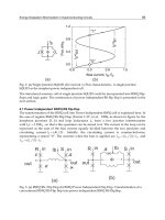
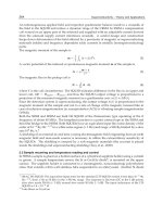
system is affected by the parameter variation. Compared with the nominal system, the
position trajectory is different, bigger overshoot and the relative stability degrades.
In summery, the robust optimal SMC system owns the optimal performance and global
robustness to uncertainties.

0 5 10 15 20
0
0.2
0.4
0.6
0.8
1
time(sec)
position
Robust Optimal SMC
Optimal Control

(a) Position responses

0 5 10 15 20
0
0.1
0.2
0.3
0.4
0.5
0.6

0.7
0.8
time(sec)
J(t)
Robust Optimal SMC
Optimal Control

(b) Performance indexes
Fig. 2. Simulation results in Case 2
2.4 Conclusion
In this section, the integral sliding mode control strategy is applied to robustifying the
optimal controller. An optimal robust sliding surface is designed so that the initial condition
is on the surface and reaching phase is eliminated. The system is global robust to
uncertainties which satisfy matching conditions and the sliding motion minimizes the given
quadratic performance index. This method has been adopted to control the rotor position of
an electrical servo drive. Simulation results show that the robust optimal SMCs are superior
to optimal LQR controllers in the robustness to parameter variations and external
disturbances.
Robust Control, Theory and Applications

148
3. Optimal sliding mode control for uncertain nonlinear system
In the section above, the robust optimal SMC design problem for a class of uncertain linear
systems is studied. However, nearly all practical systems contain nonlinearities, there would
exist some difficulties if optimal control is applied to handling nonlinear problems (Chiou &
Huang, 2005; Ho, 2007, Cimen & Banks, 2004; Tang et al., 2007).In this section, the global
robust optimal sliding mode controller (GROSMC) is designed based on feedback
linearization for a class of MIMO uncertain nonlinear system.
3.1 Problem formulation
Consider an uncertain affine nonlinear system in the form of

() () (,),
(),
xfx gxudtx
yHx
=+ +
=

(19)
where
n
xR∈
is the state,
m
uR∈
is the control input, and ()
f
x and ()gx are sufficiently
smooth vector fields on a domain
n
DR⊂ .Moreover, state vector x is assumed available,
()Hx is a measured sufficiently smooth output function and
T
1
() ( , , )
m
Hx h h=  . (, )dtx is an
unknown function vector, which represents the system uncertainties, including system
parameter variations, unmodeled dynamics and external disturbances.
Assumption 5. There exists an unknown continuous function vector (, )tx

δ
such that (, )dtx
can be written as
(, ) ( ) (, )dtx gx tx
δ
=
.
This is called matching condition.
Assumption 6. There exist positive constants
0
γ
and
1
γ
, such that
01
(, )tx x
δγγ
≤+
where the notation
⋅
denotes the usual Euclidean norm.
By setting all the uncertainties to zero, the nominal system of the uncertain system (19) can
be described as

() () ,
().
xfx gxu
yHx
=+

=

(20)
The objective of this paper is to synthesize a robust sliding mode optimal controller so that
the uncertain affine nonlinear system has not only the optimal performance of the nominal
system but also robustness to the system uncertainties. However, the nominal system is
nonlinear. To avoid the nonlinear TPBV problem and approximate linearization problem,
we adopt the feedback linearization to transform the uncertain nonlinear system (19) into an
equivalent linear one and an optimal controller is designed on it, then a GROSMC is
proposed.
3.2 Feedback linearization
Feedback linearization is an important approach to nonlinear control design. The central
idea of this approach is to find a state transformation
()zTx
=
and an input transformation
Optimal Sliding Mode Control for a Class of
Uncertain Nonlinear Systems Based on Feedback Linearization

149
(,)uuxv= so that the nonlinear system dynamics is transformed into an equivalent linear
time-variant dynamics, in the familiar form zAzBv
=
+

, then linear control techniques can
be applied.
Assume that system (20) has the vector relative degree
{
}

1
,,
m
rr
and
1 m
rrn++= .
According to relative degree definition, we have

()
() 1
1
,0 1
(),
ii i
k
k
fi i
i
m
rr r
i
j
i
j
i
ff
j
yLh kr
y

Lh g L h u
−
=
=≤≤−
=+
∑
(21)
and the decoupled matrix
11
1
1
11
11
11
() ()
() ( )
() ()
m
mm
m
rr
gg
ff
ij m m
rr
gm g m
ff
LLh LLh
Ex e
LL h L L h

−−
×
−−
⎡
⎤
⎢
⎥
⎢
⎥
==
⎢
⎥
⎢
⎥
⎣
⎦





is nonsingular in some domain
0
xX∀∈
.
Choose state and input transformations as follows:

() ,1,,;0,1,,1
jj j
ii

ii
f
zTxLhi mj r
=
== = −
(22)

1
()[ ()],uE xvKx
−
=− (23)
where
1
T
1
() ( , , )
m
r
r
m
ff
Kx Lh L h= 
, v is an equivalent input to be designed later. The uncertain
nonlinear system (19) can be transformed into m subsystems; each one is in the form of

00
11
11
1
0

010 0 0
0
001 0 0
.
0
000 1 0
000 0 1
ii
i
ii
ii
i
rr
r
ii
di
f
zz
zz
v
zz
LL h
−−
−
⎡
⎤
⎡⎤⎡⎤
⎡⎤ ⎡⎤
⎢
⎥

⎢⎥⎢⎥
⎢⎥ ⎢⎥
⎢
⎥
⎢⎥⎢⎥
⎢⎥ ⎢⎥
⎢
⎥
⎢⎥⎢⎥
=++
⎢⎥ ⎢⎥
⎢
⎥
⎢⎥⎢⎥
⎢⎥ ⎢⎥
⎢
⎥
⎢⎥⎢⎥
⎢⎥ ⎢⎥
⎢
⎥
⎢⎥⎢⎥
⎣⎦ ⎣⎦
⎣⎦⎣⎦
⎢
⎥
⎣
⎦






   




(24)
So system (19) can be transformed into the following equivalent model of a simple linear
form:
() () () (, ),zt Azt Bvt tz
ω
=++

(25)
where
n
zR∈ ,
m
vR∈ are new state vector and input, respectively.
nn
A
R
×
∈
and
nm
BR
×

∈
are constant matrixes, and (,)AB are controllable. ( , )
n
tz R
ω
∈ is the uncertainties of the
equivalent linear system. As we can see, (,)tz
ω
also satisfies the matching condition, in
other words there exists an unknown continuous vector function (,)tz
ω

such that
(, ) (, )tz B tz
ω
ω
=

.
Robust Control, Theory and Applications

150
3.3 Design of GROSMC
3.3.1 Optimal control for nominal system
The nominal system of (25) is

() () ().zt Azt Bvt
=
+


(26)
For (26), let
0
vv=
and
0
v
can minimize a quadratic performance index as follows:

TT
00
0
1
[()() () ()]
2
JztQztvtRvtdt
∞
=+
∫
(27)
where
nn
QR
×
∈ is a symmetric positive definite matrix,
mm
RR
×
∈ is a positive definite
matrix. According to optimal control theory, the optimal feedback control law can be

described as

1T
0
() ()vt RBPzt
−
=− (28)
with
P the solution of the matrix Riccati equation

T1T
0.PA A P PBR B P Q
−
+
−+=
(29)
So the closed-loop dynamics is

1T
() ( )().zt A BR B Pzt
−
=−

(30)
The closed-loop system is asymptotically stable.
The solution to equation (30) is the optimal trajectory z*(t) of the nominal system with
optimal control law (28). However, if the control law (28) is applied to uncertain system (25),
the system state trajectory will deviate from the optimal trajectory and even the system
becomes unstable. Next we will introduce integral sliding mode control technique to
robustify the optimal control law, to achieve the goal that the state trajectory of uncertain

system (25) is the same as that of the optimal trajectory of the nominal system (26).
3.3.2 The optimal sliding surface
Considering the uncertain system (25) and the optimal control law (28), we define an
integral sliding surface in the form of

1T
0
() [() (0)] ( )( )
t
st Gzt z G A BR B Pz d
τ
τ
−
=−− −
∫
(31)
where
mn
GR
×
∈ , which satisfies that GB is nonsingular, (0)z is the initial state vector.
Differentiating (31) with respect to
t and considering (25), we obtain

1T
1T
1T
() () ( )()
[() () (,)] ( )()
() () (, )

st Gzt GA BR B Pzt
GAzt Bvt tz GA BR B Pzt
GBv t GBR B Pz t G t z
ω
ω
−
−
−
=−−
=++−−
=+ +

(32)
Let
() 0st =

, the equivalent control becomes
Optimal Sliding Mode Control for a Class of
Uncertain Nonlinear Systems Based on Feedback Linearization

151

11T
eq
() ( ) () (, )vt GB GBRBPzt Gtz
ω
−−
⎡
⎤
=− +

⎣
⎦
(33)
Substituting (33) into (25), the sliding mode dynamics becomes

11T
1T 1
1T 1
1T
()( )
()
()
()
z Az B GB GBR B Pz G
Az BR B Pz B GB G
Az BR B Pz B GB GB B
ABRBPz
ω
ω
ωω
ω
ω
−
−
−−
−−
−
=
−++
=− − +

=− − +
=−


(34)
Comparing (34) with (30), we can see that the sliding mode of uncertain linear system (25) is
the same as optimal dynamics of (26), thus the sliding mode is also asymptotically stable,
and the sliding motion guarantees the controlled system global robustness to the uncertainties
which satisfy the matching condition. We call (31) a global robust optimal sliding surface.
Substituting state transformation
()zTx= into (31), we can get the optimal switching
function
(,)sxt in the x -coordinates.
3.3.3 The control law
After designing the optimal sliding surface, the next step is to select a control law to ensure
the reachability of sliding mode in finite time.
Differentiating
(,)sxt
with respect to t and considering system (20), we have

(() ()) .
sss s
sx fxgxu
xtx t
∂
∂∂ ∂
=+= + +
∂
∂∂ ∂


(35)
Let 0s =

, the equivalent control of nonlinear nominal system (20) is obtained

1
() ( ) ( ) .
eq
sss
ut gx fx
xxt
−
∂
∂∂
⎡
⎤⎡ ⎤
== − +
⎢
⎥⎢ ⎥
∂
∂∂
⎣
⎦⎣ ⎦
(36)
Considering equation (23), we have
1
0
()[ ()]
eq
uExvKx

−
=−.
Now, we select the control law in the form of

con dis
1
con
1
dis 0 1
() () (),
() () () ,
() ( ) ( ( ) ( ))s
g
n( ),
ut u t u t
sss
ut gx fx
xxt
ss
ut gx x gx s
xx
ηγ γ
−
−
=+
∂∂∂
⎡⎤⎡ ⎤
== − +
⎢⎥⎢ ⎥
∂∂∂

⎣⎦⎣ ⎦
∂∂
⎡⎤
=− + +
⎢⎥
∂∂
⎣⎦
(37)
where
[]
T
12
s
g
n( ) s
g
n( ) s
g
n( ) s
g
n( )
m
sss s=  and
0
η
>
.
con
()ut and
dis

()ut denote
continuous part and discontinuous part of
()ut , respectively.
The continuous part
con
()ut
, which is equal to the equivalent control of nominal system (20),
is used to stabilize and optimize the nominal system. The discontinuous part
dis
()ut
provides the complete compensation of uncertainties for the uncertain system (19).
Theorem 2. Consider uncertain affine nonlinear system (19) with Assumputions 5-6. Let
u and sliding surface be given by (37) and (31), respectively. The control law can force the
system trajectories to reach the sliding surface in finite time and maintain on it thereafter.
Robust Control, Theory and Applications

152
Proof.
Utilizing
T
(1/2)Vss= as a Lyapunov function candidate, and taking the Assumption 5
and Assumption 6, we have
TT
T
01
TT T
01 01
11
01
1

(( ) )
()sgn()
()sgn() ()
()
ss
Vsss f gud
xt
sss s ss
sf f xg s d
xxt x xt
ss ss
sxgssdsxgssg
xx xx
s
sx
x
ηγ γ
η
γγ η γγ δ
ηγγ
∂∂
== +++=
∂∂
⎧
⎡⎤
⎛⎞∂∂∂ ∂ ∂∂
⎪
⎫
=−++++ ++=
⎨⎬

⎢⎥
⎜⎟
∂∂∂ ∂ ∂∂
⎭
⎝⎠
⎪
⎣⎦
⎩
⎧⎫
⎡⎤∂∂ ∂∂
⎪⎪
=−++ + =− −+ +
⎨⎬
⎢⎥
∂∂ ∂∂
⎪⎪
⎣⎦
⎩⎭
∂
≤− − +
∂


1
01 01
11
() ()
s
gs gs
x

ss
sxgsxgs
xx
δ
ηγγ γγ
∂
+≤
∂
∂∂
≤− − + + +
∂∂
(38)
where
1
i denotes the 1-norm. Noting the fact that
1
ss≥ , we get

T
0,for 0.Vss s s
η
=
≤− < ≠


(39)
This implies that the trajectories of the uncertain nonlinear system (19) will be globally
driven onto the specified sliding surface 0s
=
despite the uncertainties in finite time. The

proof is complete.
From (31), we have
(0) 0s
=
, that is the initial condition is on the sliding surface. According
to Theorem2, we know that the uncertain system (19) with the integral sliding surface (31)
and the control law (37) can achieve global sliding mode. So the system designed is global
robust and optimal.
3.4 A simulation example
Inverted pendulum is widely used for testing control algorithms. In many existing
literatures, the inverted pendulum is customarily modeled by nonlinear system, and the
approximate linearization is adopted to transform the nonlinear systems into a linear one,
then a LQR is designed for the linear system.
To verify the effectiveness and superiority of the proposed GROSMC, we apply it to a single
inverted pendulum in comparison with conventional LQR.
The nonlinear differential equation of the single inverted pendulum is

12
2
1211 1
2
2
1
,
sin sin cos cos
(),
(4/3 cos )
xx
gxamLx x xaux
xdt

Lamx
=
−+
=+
−


(40)
where
1
x
is the angular position of the pendulum
(rad)
,
2
x
is the angular speed
(rad/s)
,
M
is the mass of the cart, m and L are the mass and half length of the pendulum,
respectively. u denotes the control input,
g
is the gravity acceleration, ()dt represents the
external disturbances, and the coefficient
/( )am Mm=+
. The simulation parameters are as
follows:
1k
g

M = , 0.2 k
g
m
=
, 0.5 mL
=
,
2
9.8 m/sg = , and the initial state vector is
T
(0) [ /18 0]x
π
=− .
Optimal Sliding Mode Control for a Class of
Uncertain Nonlinear Systems Based on Feedback Linearization

153
Two cases with parameter variations in the inverted pendulum and external disturbance are
considered here.
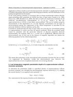
Case 1: The m and L are 4 times the parameters given above, respectively. Fig. 3 shows the
robustness to parameter variations by the suggested GROSMC and conventional
LQR.
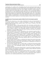
Case 2: Apply an external disturbance
( ) 0.01sin 2dt t
=
to the inverted pendulum system at

9ts= . Fig. 4 depicts the different responses of these two controllers to external
disturbance.

0 2 4 6 8 10
-0.18
-0.16
-0.14
-0.12
-0.1
-0.08
-0.06
-0.04
-0.02
0
0.02
t (s)
Angular Position x1 (t)
m=0.2 kg,L=0.5 m
m=0.8 kg,L=2 m
0 2 4 6 8 10
-0.18
-0.16
-0.14
-0.12
-0.1
-0.08
-0.06
-0.04
-0.02
0
0.02
t (s)
Angular Position x1(t)

m=0.2 kg,L=0.5 m
m=0.8 kg,L=2 m

(a) By GROSMC (b) By Conventional LQR.
Fig. 3. Angular position responses of the inverted pendulum with parameter variation

0 5 10 15 20
-0.18
-0.16
-0.14
-0.12
-0.1
-0.08
-0.06
-0.04
-0.02
0
0.02
t (s)
angular position x1 (t)
Optimal Control
GROSMC

Fig. 4. Angular position responses of the inverted pendulum with external disturbance.
From Fig. 3 we can see that the angular position responses of inverted pendulum with and
without parameter variations are exactly same by the proposed GROSMC, but the responses
are obviously sensitive to parameter variations by the conventional LQR. It shows that the
proposed GROSMC guarantees the controlled system complete robustness to parameter
variation. As depicted in Fig. 4, without external disturbance, the controlled system could be
driven to the equilibrium point by both of the controllers at about

2ts
=
. However, when
the external disturbance is applied to the controlled system at
9ts
=
, the inverted
pendulum system could still maintain the equilibrium state by GROSMC while the LQR not.
Robust Control, Theory and Applications

154
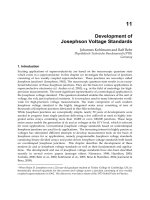
The switching function curve is shown in Fig. 5. The sliding motion occurs from the
beginning without any reaching phase as can be seen. Thus, the GROSMC provides better
features than conventional LQR in terms of robustness to system uncertainties.

0 5 10 15 20
-0.5
-0.4
-0.3
-0.2
-0.1
0
0.1
0.2
0.3
0.4
0.5
t (s)
s (t)
Sliding Surface

Fig. 5. The switching function s(t)
3.5 Conclusion
In this section, the exact linearization technique is firstly adopted to transform an uncertain
affine nonlinear system into a linear one. An optimal controller is designed to the linear
nominal system, which not only simplifies the optimal controller design, but also makes the
optimal control applicable to the entire transformation region. The sliding mode control is
employed to robustfy the optimal regulator. The uncertain system with the proposed
integral sliding surface and the control law achieves global sliding mode, and the ideal
sliding dynamics can minimized the given quadratic performance index. In summary, the
system designed is global robust and optimal.
4. Optimal sliding mode tracking control for uncertain nonlinear system
With the industrial development, there are more and more control objectives about the
system tracking problem (Ouyang et al., 2006; Mauder, 2008; Smolders et al., 2008), which is
very important in control theory synthesis. Taking the robot as an example, it is often
required to follow some special trajectories quickly as well as provide robustness to system
uncertainties, including unmodeled dynamics, internal parameter variations and external
disturbances. So the main tracking control problem becomes how to design the controller,
which can not only get good tracking performance but also reject the uncertainties
effectively to ensure the system better dynamic performance. In this section, a robust LQR
tracking control based on intergral sliding mode is proposed for a class of nonlinear
uncertain systems.
4.1 Problem formulation and assumption
Consider a class of uncertain affine nonlinear systems as follows:

() () ()[ (,,)]
()
xfx fx gxu xtu
yhx
δ

=+Δ+ +
⎧
⎨
=
⎩

(41)
Optimal Sliding Mode Control for a Class of
Uncertain Nonlinear Systems Based on Feedback Linearization

155
where
n
xR∈ is the state vector,
m
uR∈ is the control input with 1m
=
, and yR∈ is the
system output.
()
f
x , ()gx , ()
f
x
Δ
and ()hx are sufficiently smooth in domain
n
DR⊂ .
(,,)xtu
δ

is continuous with respect to t and smooth in
(,)xu
.
()fxΔ
and
(,,)xtu
δ
represent
the system uncertainties, including unmodelled dynamics, parameter variations and
external disturbances.
Our goal is to design an optimal LQR such that the output
y
can track a reference
trajectory
r
()yt asymptotically, some given performance criterion can be minimized, and the
system can exhibit robustness to uncertainties.
Assumption 7. The nominal system of uncertain affine nonlinear system (41), that is

() ()
()
x
f
x
g
xu
yhx
=
+
⎧

⎨
=
⎩

(42)
has the relative degree
ρ
in domain D and n
ρ
= .
Assumption 8. The reference trajectory
r
()
y
t
and its derivations
()
r
()
i
y
t
(1,,)in= 
can be
obtained online, and they are limited to all 0t ≥ .
While as we know, if the optimal LQR is applied to nonlinear systems, it often leads to
nonlinear TPBV problem and an analytical solution generally does not exist. In order to
simplify the design of this tracking problem, the input-output linearization technique is
adopted firstly.
Considering system (41) and differentiating

y
, we have
()
(), 0 1
k
k
f
yLhx kn
=
≤≤−

()
11
() () ()[ (,,)].
n
nn n
fff gf
y
LhxLLhxLLhxu xtu
δ
−
−
Δ
=+ + +

According to the input-out linearization, choose the following nonlinear state transformation

T
1
() () () .

n
f
zTx hx L hx
−
⎡
⎤
==
⎣
⎦

(43)
So the uncertain affine nonlinear system (40) can be written as
1
11
,1,,1
() () ()[ (,,)].
ii
nn n
nf ff gf
zz i n
z Lhx L L hx LL hx u xtu
δ
+
−−
Δ
=
=−
=+ + +





Define an error state vector in the form of
1r
(1)
r
,
n
n
zy
ez
zy
−
⎡⎤
−
⎢⎥
=
=−ℜ
⎢⎥
⎢⎥
−
⎣
⎦


where
T
(1)
rr
n

yy
−
⎡⎤
ℜ=
⎣⎦

. By this variable substitution ez
=
−ℜ, the error state equation
can be described as follows:
1
()
11 1
r
,1,,1
() () ()() ()(,,) ().
ii
n
nn n n
nf ff gf gf
ee i n
e Lhx L L hx LL hxut LL hx xtu
y
t
δ
+
−− −
Δ
==−
=+ + + −





Robust Control, Theory and Applications

156
Let the feedback control law be selected as

()
r
1
() () ()
()
()
n
n
f
n
gf
Lhx vt
y
t
ut
LL hx
−
−++
=
(44)
The error equation of system (40) can be given in the following forms:

11
00
010 0 0
00
001 0 0
00
0
() () () .
000 1
000 0 0 1
() ()(,,)
nn
ff gf
et et vt
L L hx LL hx xtu
δ
−−
Δ
⎡
⎤⎡ ⎤
⎡⎤ ⎡⎤
⎢
⎥⎢ ⎥
⎢⎥ ⎢⎥
⎢
⎥⎢ ⎥
⎢⎥ ⎢⎥
⎢
⎥⎢ ⎥

⎢⎥ ⎢⎥
=+++
⎢
⎥⎢ ⎥
⎢⎥ ⎢⎥
⎢
⎥⎢ ⎥
⎢⎥ ⎢⎥
⎢
⎥⎢ ⎥
⎢⎥ ⎢⎥
⎣⎦ ⎣⎦
⎣
⎦⎣ ⎦



 


(45)
Therefore, equation (45) can be rewritten as

() () () .et Aet A Bvt
δ
=
+Δ + +Δ

(46)
where

010 0 0
001 0 0
0
,,
000 1
000 0 0 1
AB
⎡
⎤⎡⎤
⎢
⎥⎢⎥
⎢
⎥⎢⎥
⎢
⎥⎢⎥
==
⎢
⎥⎢⎥
⎢
⎥⎢⎥
⎢
⎥⎢⎥
⎣
⎦⎣⎦


 


11

00
00
00
,.
() ()(,,)
nn
ff gf
A
L L hx LL hx xtu
δ
δ
−−
Δ
⎡
⎤⎡ ⎤
⎢
⎥⎢ ⎥
⎢
⎥⎢ ⎥
⎢
⎥⎢ ⎥
Δ= Δ=
⎢
⎥⎢ ⎥
⎢
⎥⎢ ⎥
⎢
⎥⎢ ⎥
⎣
⎦⎣ ⎦



As can be seen,
n
eR∈ is the system error vector, vR
∈
is a new control input of the
transformed system.
nn
A
R
×
∈
and
nm
BR
×
∈
are corresponding constant matrixes.
AΔ and
δ
Δ represent uncertainties of the transformed system.
Assumption 9. There exist unknown continuous function vectors of appropriate dimensions
A
Δ

and
δ
Δ


, such that
A
BA
Δ
=Δ

,
B
δ
δ
Δ=Δ



Assumption 10. There exist known constants
m
a ,
m
b such that
m
A
aΔ≤

,
m
b
δ
Δ≤


Now, the tracking problem becomes to design a state feedback control law
v
such that
0
e → asymptotically. If there is no uncertainty, i.e.
(,) 0te
δ
=
, we can select the new input
as
vKe=− to achieve the control objective and obtain the closed loop dynamics
()eABKe=−

. Good tracking performance can be achieved by choosing K using optimal
Optimal Sliding Mode Control for a Class of
Uncertain Nonlinear Systems Based on Feedback Linearization

157
control theory so that the closed loop dynamics is asymptotically stable. However, in
presence of the uncertainties, the closed loop performance may be deteriorated. In the
next section, the integral sliding mode control is adopted to robustify the optimal control
law.
4.2 Design of optimal sliding mode tracking controller
4.2.1 Optimal tracking control of nominal system.
Ignoring the uncertainties of system (46), the corresponding nominal system is

() () ().et Aet Bvt
=
+


(47)
For the nominal system (47), let
0
vv
=
and
0
v
can minimize the quadratic performance
index as follows:

TT
00
0
1
[()() () ()]
2
IetQetvtRvtdt
∞
=+
∫
(48)
where
nn
QR
×
∈ is a symmetric positive definite matrix,
mm
RR
×

∈
(here 1m
=
) is a positive
definite matrix.
According to optimal control theory, an optimal feedback control law can be obtained as:

1T
0
() ()vt RBPet
−
=−
(49)
with
P the solution of matrix Riccati equation
T1T
0.PA A P PBR B P Q
−
+
−+=

So the closed-loop system dynamics is

1T
() ( )().et A BR B Pet
−
=−

(50)
The designed optimal controller for system (47) is sensitive to system uncertainties

including parameter variations and external disturbances. The performance index (48) may
deviate from the optimal value. In the next part, we will use integral sliding mode control
technique to robustify the optimal control law so that the uncertain system trajectory could
be same as nominal system.
4.2.2 The robust optimal sliding surface.
To get better tracking performance, an integral sliding surface is defined as

1T
0
(,) () ( )() (0),
t
set Get G A BR BPe d Ge
ττ
−
=− − −
∫
(51)
where
mn
GR
×
∈ is a constant matrix which is designed so that GB is nonsingular. And (0)e
is the initial error state vector.
Differentiating (51) with respect to
t and considering system (46), we obtain

1T
1T
1T
(,) () ( )()

[() () ] ( )()
() () ( ).
set Get GA BR B Pet
GAet A Bvt GA BR B Pet
GBv t GBR B Pe t G A
δ
δ
−
−
−
=−−
=+Δ++Δ−−
=+ +Δ+Δ

(52)
Robust Control, Theory and Applications

158
Let (,) 0set =

, the equivalent control can be obtained by

11T
eq
( ) ( ) [ ( ) ( )].v t GB GBR B Pe t G A
δ
−
−
=− + Δ +Δ
(53)

Substituting (53) into (46), and considering Assumption 10, the ideal sliding mode dynamics
becomes

eq
11T
1T 1
1T 1
1T
() () ()
() ( ) [ () ( )]
()()()[]
()()()()()
()().
et Aet A Bv t
Ae t A B GB GBR B Pe t G A
ABRBPet BGB GA A
A BR B P e t B GB GB A B A
ABRBPet
δ
δ
δ
δδ
δ
δ
−−
−−
−−
−
=
+Δ + +Δ

=
+Δ − + Δ +Δ +Δ
= − − Δ +Δ +Δ +Δ
=
− − Δ+Δ + Δ+Δ
=−



(54)
It can be seen from equation (50) and (54) that the ideal sliding motion of uncertain system
and the optimal dynamics of the nominal system are uniform, thus the sliding mode is also
asymptotically stable, and the sliding mode guarantees system (46) complete robustness to
uncertainties. Therefore, (51) is called a robust optimal sliding surface.
4.2.3 The control law.
For uncertain system (46), we propose a control law in the form of

cd
1T
c
1
d
() () (),
() (),
( ) ( ) [ sgn( )].
vt v t v t
vt RBPet
vt GB ks s
ε
−

−
=
+
=−
=− +
(55)
where
c
v is the continuous part, which is used to stabilize and optimize the nominal
system. And
d
v is the discontinuous part, which provides complete compensation for
system uncertainties.
[]
T
1
sgn( ) sgn( ) sgn( )
m
ss s= 
. k and
ε
are appropriate positive
constants, respectively.
Theorem 3. Consider uncertain system (46) with Assumption9-10. Let the input v and the
sliding surface be given as (55) and (51), respectively. The control law can force system
trajectories to reach the sliding surface in finite time and maintain on it thereafter if
mm
()adGB
ε
≥+ .

Proof: Utilizing
T
(1/2)Vss= as a Lyapunov function candidate, and considering
Assumption 9-10, we obtain
{}
()
[]
{}
TT 1T
T1T
T1T 1T
TT
1
mm mm
1
[() ( )()]
[() () ] ( )()
() s
g
n( ) ( )
s
g
n( ) ( )
() (
VsssGet GABRBPet
sGAet ABvt GABRBPet
s G A GBR B Pe t ks s G GBR B Pe t
sks sGAG ks ssGAG
ks s a d GB s ks a d
δ

εδ
ε
δε δ
εε
−
−
−−
== − −
=+Δ++Δ−−
⎡
⎤
=Δ− −+ +Δ+
⎣
⎦
=−+ +Δ+Δ=− − + Δ+Δ
≤− − + + ≤− − − +


) GB s
⎡⎤
⎣⎦

where
1
i denotes the 1-norm. Note the fact that for any 0s
≠
, we have
1
ss≥ . If
()

mm
adGB
ε
≥+ , then
Optimal Sliding Mode Control for a Class of
Uncertain Nonlinear Systems Based on Feedback Linearization

159

T
1
()0.Vss s G s G s
εδεδ
=
≤− + ≤− − <


(56)
This implies that the trajectories of uncertain system (46) will be globally driven onto the
specified sliding surface
(,) 0set
=
in finite time and maintain on it thereafter. The proof is
completed.
From (51), we have
(0) 0s
=
, that is to say, the initial condition is on the sliding surface.
According to Theorem3, uncertain system (46) achieves global sliding mode with the
integral sliding surface (51) and the control law (55). So the system designed is global robust

and optimal, good tracking performance can be obtained with this proposed algorithm.
4.3 Application to robots.
In the recent decades, the tracking control of robot manipulators has received a great of
attention. To obtain high-precision control performance, the controller is designed which
can make each joint track a desired trajectory as close as possible. It is rather difficult to
control robots due to their highly nonlinear, time-varying dynamic behavior and uncertainties
such as parameter variations, external disturbances and unmodeled dynamics. In this
section, the robot model is investigated to verify the effectiveness of the proposed method.
A 1-DOF robot mathematical model is described by the following nonlinear dynamics:

01 0
00
(),
(,) ()
11
0
() ()
() ()
qq
dt
Cqq Gq
qq
Mq Mq
Mq Mq
τ
⎡⎤⎡⎤
⎡⎤⎡⎤
⎡⎤ ⎡⎤
⎢⎥⎢⎥
⎢⎥⎢⎥

=−+−
⎢⎥ ⎢⎥
⎢⎥⎢⎥
⎢⎥⎢⎥
−
⎣⎦ ⎣⎦
⎢⎥⎢⎥
⎢⎥⎢⎥
⎣
⎦⎣ ⎦
⎣
⎦⎣⎦


 
(57)
where ,
q
q

denote the robot joint position and velocity, respectively.
τ
is the control vector
of torque by the joint actuators. m and l are the mass and length of the manipulator arm,
respectively.
()dt is the system uncertainties. (,) 0.03cos(),Cqq q=

( ) cos( ),Gq mgl q=
() 0.1 0.06sin().
M

qq=+
The reference trajectory is
r
() sin
y
tt
π
=
.
According to input-output linearization technique, choose a state vector as follows:
1
2
z
q
z
z
q
⎡
⎤⎡⎤
==
⎢
⎥⎢⎥
⎣
⎦⎣⎦

.
Define an error state vector of system (57) as
[][ ]
TT
12 r r

,eee qyqy==−−

and let the
control law
r
()()(,)()vyMq CqqqGq
τ
=+ + +
  
.
So the error state dynamic of the robot can be written as:

11
22
01 0 0
()
00 1 1/ ()
ee
vdt
ee Mq
⎡⎤⎡ ⎤⎡⎤⎡⎤ ⎡ ⎤
=+−
⎢⎥⎢ ⎥⎢⎥⎢⎥ ⎢ ⎥
⎣
⎦⎣ ⎦⎣⎦⎣⎦ ⎣ ⎦


(58)
Choose the sliding mode surface and the control law in the form of (51) and (55),
respectively, and the quadratic performance index in the form of (48). The simulation

parameters are as follows:
0.02,m
=
9.8,g
=
0.5,l
=
() 0.5sin2 ,dt t
π
=
18,k = 6,
ε
=
[
]
01,G =

10 2
,
21
Q
⎡⎤
=
⎢⎥
⎣⎦
1R
=
. The initial error state vector is
[]
T

0.5 0e =
.
The tracking responses of the joint position
qand its velocity are shown in Fig. 6 and Fig. 7,
respectively. The control input
 is displayed in Fig. 8. From Fig. 6 and Fig. 7 it can be seen
that the position error can reach the equilibrium point quickly and the position track the
Robust Control, Theory and Applications

160
reference sine signal y
r
well. Simulation results show that the proposed scheme manifest
good tracking performance and the robustness to parameter variations and the load
disturbance.
4.4 Conclusions
In order to achieve good tracking performance for a class of nonlinear uncertain systems, a
sliding mode LQR tracking control is developed. The input-output linearization is used to
transform the nonlinear system into an equivalent linear one so that the system can be
handled easily. With the proposed control law and the robust optimal sliding surface, the
system output is forced to follow the given trajectory and the tracking error can minimize
the given performance index even if there are uncertainties. The proposed algorithm is
applied to a robot described by a nonlinear model with uncertainties. Simulation results
illustrate the feasibility of the proposed controller for trajectory tracking and its capability of
rejecting system uncertainties.

0 5 10 15
-1.5
-1
-0.5

0
0.5
1
1.5
time/s
position
reference trajectory
position response
position error

Fig. 6. The tracking response of
q

0 5 10 15
-4
-3
-2
-1
0
1
2
3
4
time/s
speed
reference speed
speed response

Fig. 7. The tracking response of
q



Optimal Sliding Mode Control for a Class of
Uncertain Nonlinear Systems Based on Feedback Linearization

161
0 5 10 15
-3
-2.5
-2
-1.5
-1
-0.5
0
0.5
1
1.5
2
time/s
control input

Fig. 8. The control input
τ

5. Acknowledgements
This work is supported by National Nature Science Foundation under Grant No. 60940018.
6. References
Basin, M.; Rodriguez-Gonzaleza, J.; Fridman, L. (2007). Optimal and robust control for linear
state-delay systems.
Journal of the Franklin Institute. Vol.344, pp.830–845.

Chen, W. D.; Tang, D. Z.; Wang, H. T. (2004). Robust Tracking Control Of Robot M
anipulators Using Backstepping.
Joranal of System Simulation. Vol. 16, No. 4, pp. 837-
837, 841.
Choi, S. B.; Cheong, C. C.; Park, D. W. (1993). Moving switch surfaces for robust control of
second-order variable structure systems.
International Journal of Control. Vol.58,
No.1, pp. 229-245.
Choi, S. B.; Park, D. W.; Jayasuriya, S. (1994). A time-varying sliding surface for fast and
robust tracking control of second-order uncertain systems.
Automatica. Vol.30, No.5,
pp. 899-904.
Chiou, K. C.; Huang, S. J. (2005). An adaptive fuzzy controller for robot manipulators.
Mechatronics. Vol.15, pp.151-177.
Cimen, T.; Banks, S. P. (2004). Global optimal feedback control for general nonlinear systems
with nonquadratic performance criteria.
System & Control Letters. Vol.53, pp.327-
346.
Cimen, T.; Banks, S. P. (2004). Nonlinear optimal tracking control with application to super-
tankers for autopilot design.
Automatica. Vol.40, No.11, pp.1845 – 1863.
Gao, W. B.; Hung, J C. (1993). Variable structure control of nonlinear systems: A new
approach.
IEEE Transactions on Industrial Electronics. Vol.40, No.1, pp. 45-55.
Ho, H. F.; Wong, Y. K.; Rad, A. B. (2007). Robust fuzzy tracking control for robotic
manipulators.
Simulation Modelling Practice and Theory. Vol.15, pp.801-816.
Laghrouche, S.; Plestan, F.; Glumineau, A. (2007). Higher order sliding mode control based
on integral sliding mode.
Automatica. Vol. 43, pp.531-537.

Robust Control, Theory and Applications

162
Lee, J. H. (2006). Highly robust position control of BLDDSM using an improved integral
variable structure system.
Automatica. Vol.42, pp.929-935.
Lin, F. J.; Chou, W. D. (2003). An induction motor servo drive using sliding mode controller
with genetic algorithm.
Electric Power Systems Research. Vol.64, pp.93-108.
Mokhtari, A.; Benallegue, A.; Orlov, Y. (2006). Exact linearization and sliding mode observer
for a quadrotor unmanned aerial vehicle.
International Journal of Robotics and
Automation.
Vol. 21, No.1, pp.39-49.
Mauder, M. Robust tracking control of nonholonomic dynamic systems with application to
the bi-steerable mobile robot. (2008).
Automatica. Vol.44, No.10, pp.2588-2592.
Ouyang, P. R.; Zhang, W. J.; Madan M. Gupta. (2006). An adaptive switching learning
control method for trajectory tracking of robot manipulators.
Mechatronics. Vol.16,
No.1, pp.51-61.
Tang, G. Y.; Sun, H. Y.; Pang, H. P. (2008). Approximately optimal tracking control for
discrete time-delay systems with disturbances.
Progress in Natural Science. Vol.18,
pp. 225-231.
Pang, H. P.; Chen, X. (2009). Global robust optimal sliding mode control for uncertain affine
nonlinear systems.
Journal of Systems Engineering and Electronics. Vol.20, No.4, pp.
838-843.
Pang H. P.; Wang L.P. (2009). Global Robust Optimal Sliding Mode Control for a class of

Affine Nonlinear Systems with Uncertainties Based on SDRE.
Proceeding of 2009
Second International Workshop on Computer Science and Engineering. Vol. 2, pp. 276-
280.
Pang, H. P.; Tang, G. Y.; Sun, H.Y. (2009). Optimal Sliding Mode Design for a Class of
Uncertain Systems with Time-delay.
Information and Control. Vol.38, No.1, pp.87-92.
Tang, G. Y.; Gao, D. X. (2005). Feedforward and feedback optimal control for nonlinear
systems with persistent disturbances.
Control and Decision. Vol.20, No.4, pp. 366-
371.
Tang, G. Y. (2005). Suboptimal control for nonlinear systems: a successive approximation
approach.
Systems and Control Letters. Vol. 54, No.5, pp.429-434.
Tang, G. Y.; Zhao, Y. D.; Zhang, B. L. (2007). Optimal output tracking control for nonlinear
systems via successive approximation approach.
Nonlinear Analysis. Vol.66, No.6,
pp.1365–1377.
Shamma, J. S.; Cloutier, J. R. (2001). Existence of SDRE stabilizing feedback.
Proceedings of the
American Control Conference
. pp.4253-4257, Arlington VA.
Smolders, K.; Volckaert, M. Swevers, J. (2008). Tracking control of nonlinear lumped
mechanical continuous-time systems: A model-based iterative learning approach.
Mechanical Systems and Signal Processing. Vol.22, No.8, pp.1896–1916.
Yang K. D.; Özgüner. Ü. (1997). Sliding-mode design for robust linear optimal control.
Automatica. Vol. 33, No. 7, pp. 1313-1323.

8
Robust Delay-Independent/Dependent

Stabilization of Uncertain Time-Delay
Systems by Variable Structure Control
Elbrous M. Jafarov
Faculty of Aeronautics and Astronautics, Istanbul Technical University
Turkey

1. Introduction
It is well known that many engineering control systems such as conventional oil-chemical
industrial processes, nuclear reactors, long transmission lines in pneumatic, hydraulic and
rolling mill systems, flexible joint robotic manipulators and machine-tool systems, jet engine
and automobile control, human-autopilot systems, ground controlled satellite and
networked control and communication systems, space autopilot and missile-guidance
systems, etc. contain some time-delay effects, model uncertainties and external disturbances.
These processes and plants can be modeled by some uncertain dynamical systems with state
and input delays. The existence of time-delay effects is frequently a source of instability and
it degrades the control performances. The stabilization of systems with time-delay is not
easier than that of systems without time-delay. Therefore, the stability analysis and
controller design for uncertain systems with delay are important both in theory and in
practice. The problem of robust stabilization of uncertain time-delay systems by various
types of controllers such as PID controller, Smith predictor, and time-delay controller,
recently, sliding mode controllers have received considerable attention of researchers.
However, in contrast to variable structure systems without time-delay, there is relatively no
large number of papers concerning the sliding mode control of time-delay systems.
Generally, stability analysis can be divided into two categories: delay-independent and
delay-dependent. It is worth to mention that delay-dependent conditions are less
conservative than delay-independent ones because of using the information on the size of
delays, especially when time-delays are small. As known from (Utkin, 1977)-(Jafarov, 2009)
etc. sliding mode control has several useful advantages, e.g. fast response, good transient
performance, and robustness to the plant parameter variations and external disturbances.
For this reason, now, sliding mode control is considered as an efficient tool to design of

robust controllers for stabilization of complex systems with parameter perturbations and
external disturbances. Some new problems of the sliding mode control of time-delay
systems have been addressed in papers (Shyu & Yan, 1993)-(Jafarov, 2005). Shyu and Yan
(Shyu & Yan, 1993) have established a new sufficient condition to guarantee the robust
stability and β-stability for uncertain systems with single time-delay. By these conditions a
variable structure controller is designed to stabilize the time-delay systems with
uncertainties. Koshkoei and Zinober (Koshkouei & Zinober, 1996) have designed a new
Robust Control, Theory and Applications

164
sliding mode controller for MIMO canonical controllable time-delay systems with matched
external disturbances by using Lyapunov-Krasovskii functional. Robust stabilization of
time-delay systems with uncertainties by using sliding mode control has been considered by
Luo, De La Sen and Rodellar (Luo et al., 1997). However, disadvantage of this design
approach is that, a variable structure controller is not simple. Moreover, equivalent control
term depends on unavailable external disturbances. Li and DeCarlo (Li & De Carlo, 2003)
have proposed a new robust four terms sliding mode controller design method for a class
of multivariable time-delay systems with unmatched parameter uncertainties and matched
external disturbances by using the Lyapunov-Krasovskii functional combined by LMI’s
techniques. The behavior and design of sliding mode control systems with state and input
delays are considered by Perruquetti and Barbot (Perruquetti & Barbot, 2002) by using
Lyapunov-Krasovskii functional.
Four-term robust sliding mode controllers for matched uncertain systems with single or
multiple, constant or time varying state delays are designed by Gouaisbaut, Dambrine and
Richard (Gouisbaut et al., 2002) by using Lyapunov-Krasovskii functionals and Lyapunov-
Razumikhin function combined with LMI’s techniques. The five terms sliding mode
controllers for time-varying delay systems with structured parameter uncertainties have
been designed by Fridman, Gouisbaut, Dambrine and Richard (Fridman et al., 2003) via
descriptor approach combined by Lyapunov-Krasovskii functional method. In (Cao et al.,
2007) some new delay-dependent stability criteria for multivariable uncertain networked

control systems with several constant delays based on Lyapunov-Krasovskii functional
combined with descriptor approach and LMI techniques are developed by Cao, Zhong and
Hu. A robust sliding mode control of single state delayed uncertain systems with parameter
perturbations and external disturbances is designed by Jafarov (Jafarov, 2005). In survey
paper (Hung et al., 1993) the various type of reaching conditions, variable structure control
laws, switching schemes and its application in industrial systems is reported by J. Y.Hung,
Gao and J.C.Hung. The implementation of a tracking variable structure controller with
boundary layer and feed-forward term for robotic arms is developed by Xu, Hashimoto,
Slotine, Arai and Harashima(Xu et al., 1989).A new fast-response sliding mode current
controller for boost-type converters is designed by Tan, Lai, Tse, Martinez-Salamero and Wu
(Tan et al., 2007). By constructing new types of Lyapunov functionals and additional free-
weighting matrices, some new less conservative delay-dependent stability conditions for
uncertain systems with constant but unknown time-delay have been presented in (Li et al.,
2010) and its references.
Motivated by these investigations, the problem of sliding mode controller design for
uncertain multi-input systems with several fixed state delays for delay-independent and
delay-dependent cases is addressed in this chapter. A new combined sliding mode
controller is considered and it is designed for the stabilization of perturbed multi-input
time-delay systems with matched parameter uncertainties and external disturbances. Delay-
independent/dependent stability and sliding mode existence conditions are derived by
using Lyapunov-Krasovskii functional and Lyapunov function method and formulated in
terms of LMI. Delay bounds are determined from the improved stability conditions. In
practical implementation chattering problem can be avoided by using saturation function
(Hung et al., 1993), (Xu et al., 1989).
Five numerical examples with simulation results are given to illustrate the usefulness of the
proposed design method.
Robust Delay-Independent/Dependent Stabilization of
Uncertain Time-Delay Systems by Variable Structure Control

165

2. System description and assumptions
Let us consider a multi-input state time-delay systems with matched parameter uncertainties
and external disturbances described by the following state-space equation:
00 11 1
( ) ( ) ( ) ( ) ( ) ( ) ( ) ( ) ( ), t 0
NN N
xt A A xt A A xt h A A xt h But D
f
t
ΔΔ Δ
=+ ++ −++ + −+ + >



() ()xt t
φ
=
, 0ht
−
≤≤ (1)
where
()
n
xt R∈ is the measurable state vector, ( )
m
ut R∈ is the control input,
01
,, ,
N
A

AA
and B are known constant matrices of appropriate dimensions, with B of full rank,
12
max[ , , , ], 0
Ni
hhhhh=>,
12
, , ,
N
hh h are known constant time-delays, ()t
φ
is a
continuous vector–valued initial function in 0ht−≤≤ ;
01
,,,
N
A
AA
ΔΔ Δ
… and D are the
parameter uncertainties,
()t
φ
is unknown but norm-bounded external disturbances.
Taking known advantages of sliding mode, we want to design a simple suitable sliding
mode controller for stabilization of uncertain time-delay system (1).
We need to make the following conventional assumptions for our design problem.
Assumption 1:
a.
0

(,)AB is stabilizable;
b.
The parameter uncertainties and external disturbances are matched with the control
input, i.e. there exist matrices
01
(), (), (), , ()
N
EtEtEt E t… , such that:

0011
() () ; () () ; , () () ; () ()
NN
A
tBEt AtBEt AtBEt DtBEt
ΔΔ
== ==
(2)
with norm-bounded matrices:
00 11
max ( ) ; max ( ) ; ,max ( )
NN
tt t
Et Et E t
Δ
αΔα Δα
≤
≤≤

()Et
α

=

G
g
=


0
()
f
t
f
≤ (3)
where
011
,,, ,
n
g
α
αα α
and
0
f
are known positive scalars.
The control goal is to design a combined variable structure controller for robust stabilization
of time-delay system (1) with matched parameter uncertainties and external disturbances.
3. Control law and sliding surface
To achieve this goal, we form the following type of combined variable structure controller:
() () () () ()
lin eq vs r

ut u t u t u t u t
=
+++ (4)
where

() ()
lin
ut Gxt=−
(5)

[
1
011
() ( ) () ( ) ( )]
eq N N
u t CB CA x t CA x t h CA x t h
−
=− + − + + −… (6)
Robust Control, Theory and Applications

166

011.
()
() () ( ) ( )
()
vs N N
st
u t k xt k xt h k xt h
st

⎡⎤
=− + − + + −
⎣⎦
(7)

()
()
r
st
u
st
δ
=−
(8)
where
01
, , ,
N
kk k and
δ
are the scalar gain parameters to be selected; G is a design matrix;
1
()CB
−
is a non-singular mm
×
matrix. The sliding surface on which the perturbed time-delay
system states must be stable is defined as a linear function of the undelayed system states as
follows:

() ()st Cxt
Γ
=
(9)
where C is a
mn× gain matrix of full rank to be selected;
Γ
is chosen as identity mm×
matrix that is used to diagonalize the control.
Equivalent control term (6) for non-perturbed time-delay system is determined from the
following equations:

011
() () () ( ) ( ) () 0
NN
s t Cx t CA x t CA x t h CA x t h CBu t
=
=+−++−+=

(10)
Substituting (6) into (1) we have a non-perturbed or ideal sliding time-delay motion of the
nominal system as follows:

01
1
() () ( ) ( )
N
N
xt Axt Axt h A xt h=+−++−


…
(11)
where

1
01
0011
() , , , ,
N
eq eq eq N eq N
CB C G A BGA A A BGA A A BGA A
−
=−=−= − =
(12)
Note that, constructed sliding mode controller consists of four terms:
1.
The linear control term is needed to guarantee that the system states can be stabilized
on the sliding surface;
2.
The equivalent control term for the compensation of the nominal part of the perturbed
time-delay system;
3.
The variable structure control term for the compensation of parameter uncertainties of
the system matrices;
4.
The min-max or relay term for the rejection of the external disturbances.
Structure of these control terms is typical and very simple in their practical implementation.
The design parameters
01 ,
, , , , ,

N
GCk k k
δ
of the combined controller (4) for delay-
independent case can be selected from the sliding conditions and stability analysis of the
perturbed sliding time-delay system.
However, in order to make the delay-dependent stability analysis and choosing an
appropriate Lyapunov-Krasovskii functional first let us transform the nominal sliding time-
delay system (11) by using the Leibniz-Newton formula. Since x(t) is continuously
differentiable for t
≥ 0, using the Leibniz-Newton formula, the time-delay terms can be
presented as:

1
1
()() (), ,( )() ()
N
tt
N
th th
xt h xt x d xt h xt x d
θ
θθθ
−−
−= − − = −
∫∫

(13)
Robust Delay-Independent/Dependent Stabilization of
Uncertain Time-Delay Systems by Variable Structure Control

167
Then, the system (11) can be rewritten as

1
01 1
( ) ( ) ( ) ( ) ( )
N
tt
N
N
th th
xt A A A xt A x d A x d
θ
θθθ
−−
=+++ − −−
∫∫

(14)
Substituting again (11) into (14) yields:
1
11 1
01 1 0 1 1
011
2
01 10 1 1 1
( ) ( ) ( ) ( ) ( ) ( )
( ) ( ) ( )
( ) ( ) ( ) ( ) ( )

N
t
NNN
th
t
NNN
th
tt t
N NN
th th th
xt A A A xt A Ax Ax h A x h d
AAxAxh Axhd
A
A A xt AA x d A x h d AA x h d
θθ θθ
θθ θθ
θ
θθθ θθ
−
−
−− −
⎡⎤
=+++ − + −++ −
⎣⎦
⎡⎤
−− + − ++ −
⎣⎦
=+++ − − − −− −
∫

∫
∫∫ ∫

2
011
( ) ( ) ( )
NN N
tt t
NN NN
th th th
AA x d AA x h d A x h d
θ
θθθ θθ
−− −
−− − − −− −
∫∫ ∫
(15)
Then in adding to (15) the perturbed sliding time-delay system with control action (4) or
overall closed loop system can be formulated as:

11
1
2
01 10 1 1
1011
2
0
11
01
() ( ) () ( ) ( )

( ) ( ) ( )
( ) ( )
() ( )
[() (
θθ θ θ
θ
θθθθθ
θθ
−−
−−−
−
=+++ − − −
−− − −− − −
−− − +Δ
+Δ − + + Δ −
−+−
∫∫
∫∫∫
∫


NN
N
tt
N
th th
ttt
NN N N
th th th
t

NN
th
NN
xt A A A xt AA x d A x h d
A
Axhd AAxdAAx hd
Axhd Axt
Axth Axth
Bk xt k xt h
1.
() ()
) ( )] ()
() ()
δ
++ − − +
NN
st st
kxth B Dft
st st
(16)
where
00
AABG=−

, the gain matrix G can be selected such that
0
A

has the desirable
eigenvalues.

The design parameters
01 ,
, , , , ,
N
GCk k k
δ
of the combined controller (4) for delay-
dependent case can be selected from the sliding conditions and stability analysis of the
perturbed sliding time-delay system (16).
4. Robust delay-independent stabilization
In this section, the existence condition of the sliding manifold and delay-independent
stability analysis of perturbed sliding time-delay systems are presented.

4.1 Robust delay-independent stabilization on the sliding surface
In this section, the sliding manifold is designed so that on it or in its neighborhood in
different from existing methods the perturbed sliding time-delay system (1),(4) is globally
Robust Control, Theory and Applications

168
asymptotically stable with respect to state coordinates. The perturbed stability results are
formulated in the following theorem.
Theorem 1: Suppose that Assumption 1 holds. Then the multivariable time-delay
system (1) with matched parameter perturbations and external disturbances driven by
combined controller (4) and restricted to the sliding surface s(t)=0 is robustly globally
asymptotically delay-independent stable with respect to the state variables, if the
following LMI conditions and parameter requirements are satisfied:


1
001

1
1

() 0
0
() 0
T
N
N
T
T
N
N
A P PA R R PA PA
PA R
H
PA R
⎡⎤
++++
⎢⎥
⎢⎥
−
=
<
⎢⎥
⎢⎥
⎢⎥
−
⎣⎦
…


(17)

0
T
CB B PB
=
> (18)

0011
; ; ;
NN
kk k
α
αα
=
== (19)

o
f
δ
≥ (20)
where
1
,,
N
PR R…
are some symmetric positive definite matrices which are a feasible
solution of LMI (17) with (18);


00
A
ABG=−
in which a gain matrix G can be assigned by
pole placement such that
0
A

has some desirable eigenvalues.
Proof: Choose a Lyapunov-Krasovskii functional candidate as follows:

1
() () ( ) ( )
i
t
N
TT
i
i
th
VxtPxt x Rx d
θ
θθ
=
−
=+
∑
∫
(21)
The time-derivative of (21) along the state trajectories of time-delay system (1), (4) can be

calculated as follows:
[
]
011 0 11
1111
01
1
2() () ( ) ( ) () ( )
( ) ( ) ( )
()()()() ()()( )( )
2() ()2() ( )
T
NN
NN
TT T T
NNNN
TT
V x tP Axt Axt h A xt h Axt Axt h
Axt h But Dft
xtRxt xthRxth xtRxt xthRxth
xtPAxt xtPAxth
ΔΔ
Δ
=+−++−++−
++ − + +
+−−−++ −−−
=+−+

0
11

011.
1
.2 () ( )2 () ()
2() ( ) 2() ( )
()
2 ( ) [ ( ) ( ) ( ) ]
()
()
2() ()2 () 2() ()
()
()( )() (
TT
N
N
TT
NN
T
NN
TTT
TT
N
xtPAxth xtPBExt
x t PBE x t h x t PBE x t h
st
x tPBk xt k xt h k xt h
st
st
x t PBGx t x t PB x t PBEf t
st
xtR R xt x

δ
+−+
+−++ −
−+−++−
−− +
+++−…
11 1
)( ) ( ) ( )
T
NN N
thRxth xthRxth−−−−− −…

Since () ()
TT
xtPBst= , then we obtain:
Robust Delay-Independent/Dependent Stabilization of
Uncertain Time-Delay Systems by Variable Structure Control

169

001
1
1
11 1 1
011
01
() ]()
2() ( ) 2() ( )
()() ()( )
2 () () 2 () ( ) 2 () ( )

2()()2()[ ()
T
T
N
TT
N
N
TT
NN
TT T
NN
TT
VxtAPPA R Rxt
xtPAxth xtPAxth
xthRxth xthRxth
s tExt s tExt h s tE xt h
stEft stkxt k
⎡
≤++++
⎢
⎣
+−++ −
−− −−−− −
++−++−
+− +

…

1.
1

001
1 1
1
1
00
() ()
() ( )] 2()
() ()

() ()
() ()
() 0
()
()
() 0
[( ) (
T
NN
T
T
N
N
T
N
N
T
N
N
st st
xt h k xt h s t

st st
A P PA R R PA PA
xt xt
xt h xt h
PA R
xt h
xt h
PA R
kxt
δ
α
−++ − −
⎡⎤
⎡
++++
⎡⎤⎡⎤
⎢⎥
⎢
⎣
⎢⎥⎢⎥
⎢⎥
−−
⎢⎥
⎢⎥
−
⎢⎥
≤
⎢⎥
⎢⎥
⎢⎥

⎢⎥
⎢⎥
⎢⎥
−
−
⎣⎦
⎣⎦
⎢⎥
−
⎣⎦
−−
…


11 1
0
)()( )( )() ( )( )()]
()()
NN N
st k xt h st k xt h st
fst
αα
δ
+− − ++ − −
−−
(22)
Since (17)-(20) hold, then (22) reduces to:
() () 0
T
VztHzt

≤
<

(23)
where
[
]
1
() () ( ) ( )
T
N
z t xt xt h xt h=− −… .
Therefore, we can conclude that the perturbed time-delay system (1), (4) is robustly globally
asymptotically delay-independent stable with respect to the state coordinates. Theorem 1 is
proved.
4.2 Existence conditions
The final step of the control design is the derivation of the sliding mode existence conditions
or the reaching conditions for the perturbed time-delay system (1),(4) states to the sliding
manifold in finite time. These results are summarized in the following theorem.
Theorem 2: Suppose that Assumption 1 holds. Then the perturbed multivariable time-
delay system (1) states with matched parameter uncertainties and external disturbances
driven by controller (4) converge to the siding surface s(t)=0 in finite time, if the
following conditions are satisfied:

00 11
; ; ;
NN
kgk k
α
αα

=
+= = (24)

o
f
δ
≥ (25)
Proof: Let us choose a modified Lyapunov function candidate as:

1
1
()( ) ()
2
T
VstCBst
−
=
(26)
The time-derivative of (26) along the state trajectories of time-delay system (1), (4) can be
calculated as follows:
Robust Control, Theory and Applications

170

[
]
[
11
1
011

011
1
011
011
()( ) () ()( ) ()
()( ) () ( ) ( )
() ( ) ( ) () ()
()( ) () ( ) ( )
() ( )
TT
T
NN
NN
T
NN
V s tCB st s tCB Cxt
stCB CAxt Axth Axth
Axt Axt h A xt h But Df t
s t CB CA x t CA x t h CA x t h
CBE x t CBE x t h
ΔΔ Δ
−
−
−
−
==
=+−++−
++−++−++
=+−++−
++−+



[]
(
]
1
01
011.
011
011.
()
() () ( ) ( )
()
() ( ) ( )
()
()
() ()
()
()[ () ( ) ( )]
() ( ) (
NN
NN
NN
T
NN
NN
CBE x t h
CB CB CA x t CA x t h CA x t h
st
kxt kxt h k xt h

st
st
Gx t C BEf t
st
s t Ext Ext h E xt h
kxt kxt h k xt h
δ
−
+−
− + −++ −
⎡⎤
−+−++−
⎣⎦
⎞
−− +
⎟
⎟
⎠
=+−++−
−+−++−
…
]
00 11 1
0
()
)
()
()
() ()
()

[( )()()( )( )()
( ) ( ) ( ) ] ( ) ( )
NN N
st
st
st
Gx t Ef t
st
kgxtstkxthst
kxthst fst
δ
αα
αδ
⎡⎤
⎣⎦
−− +
≤− − − + − −
++ − − − −

(27)

Since (24), (25) hold, then (27) reduces to:

1
0
()( ) () ( ) () ()
T
VstCBst fst st
δη
−

=≤−−≤−


(28)
where

0
0f
ηδ
=
−≥
(29)
Hence we can evaluate that

1
min
2
() ()
()
Vt Vt
CB
η
λ
−
≤−

(30)
The last inequality (30) is known to prove the finite-time convergence of system (1), (4)
towards the sliding surface s(t)=0 (Utkin, 1977), (Perruquetti & Barbot, 2002). Therefore,
Theorem 2 is proved.

4.3 Numerical examples and simulation
In order to demonstrate the usefulness of the proposed control design techniques let us
consider the following examples.
Example 1: Consider a networked control time-delay system (1), (4) with parameters
taking from (Cao et al., 2007):

01
40 1.5 0 2
,,
13 1 0.5 2
AA B
−
−
⎡
⎤⎡ ⎤⎡⎤
== =
⎢
⎥⎢ ⎥⎢⎥
−− − −
⎣
⎦⎣ ⎦⎣⎦
(31)
Robust Delay-Independent/Dependent Stabilization of
Uncertain Time-Delay Systems by Variable Structure Control

171
001 1
0.5sin( ) , 0.5cos( ) , 0.3sin( )AtAAtAft
Δ
Δ

=
==
The LMI stability and sliding mode existence conditions are computed by MATLAB
programming (see Appendix 1) where LMI Control Toolbox is used. The computational
results are following:
A0hat =
-1.0866 1.0866
1.9134 -1.9134
⎡⎤
⎢⎥
⎣⎦
; A1hat =
-0.1811 0.1811
0.3189 -0.3189
⎡
⎤
⎢
⎥
⎣
⎦

G1 =
[
]
0.9567 1.2933 ; A0til =
-3.0000 -1.5000
0.0000 -4.5000
⎡
⎤
⎢

⎥
⎣
⎦
; eigA0til =
-3.0000
-4.5000
⎡
⎤
⎢
⎥
⎣
⎦

eigA0hat =
0.0000
-3.0000
⎡⎤
⎢⎥
⎣⎦
; eigA1hat =
0.0000
-0.5000
⎡
⎤
⎢
⎥
⎣
⎦

lhs =

-1.8137 0.0020 -0.1392 0.1392
0.0020 -1.7813 0.1382 -0.1382
-0.1392 0.1382 -1.7364 0.0010
0.1392 -0.1382 0.0010 -1.7202
⎡⎤
⎢⎥
⎢⎥
⎢⎥
⎢⎥
⎢⎥
⎣⎦
; eigsLHS =
-2.0448
-1.7952
-1.7274
-1.4843
⎡
⎤
⎢
⎥
⎢
⎥
⎢
⎥
⎢
⎥
⎢
⎥
⎣
⎦

P =
0.6308 -0.0782
-0.0782 0.3891
⎡
⎤
⎢
⎥
⎣
⎦
; eigP =
0.3660
0.6539
⎡
⎤
⎢
⎥
⎣
⎦
;
R1 =
1.7364 -0.0010
-0.0010 1.7202
⎡
⎤
⎢
⎥
⎣
⎦
; eigR1 =

1.7202
1.7365
⎡
⎤
⎢
⎥
⎣
⎦

BTP =
[
]
1.1052 0.6217 ; BTPB = 3.4538
invBTPB = 0.2895; normG1 = 1.6087
k0= 2.1087; k1=0.5;
δ
≥ 0.3; H< 0;
The networked control time-delay system is robustly asymptotically delay-independent
stable.
Example 2: Consider a time-delay system (1), (4) with parameters:
01
10.7 0.10.1
,,
0.3 1 0 0.2
AA
−
⎡
⎤⎡ ⎤
==
⎢

⎥⎢ ⎥
⎣
⎦⎣ ⎦
2
0.2 0 1
,
00.1 1
AB
⎡
⎤⎡⎤
==
⎢
⎥⎢⎥
⎣
⎦⎣⎦


1
0.1h = ,
2
0.2h = (32)
01 2
0.2sin() 0 0.1cos() 0 0.2cos() 0
,,.
0 0.1sin( ) 0 0.2cos( ) 0 0.1cos( )
tt t
AAA
ttt
ΔΔΔ
⎡⎤⎡⎤⎡⎤

== =
⎢⎥⎢⎥⎢⎥
⎣⎦⎣⎦⎣⎦

Matching condition for external disturbances is given by:
1
B 0.2cos t
1
DE
⎡⎤
==
⎢⎥
⎣⎦
; () 0.2cosft t=
The LMI stability and sliding mode existence conditions are computed by MATLAB
programming (see Appendix 2) where LMI Control Toolbox is used. The computational
results are following: