Robust Control Theory and Applications Part 6 potx

Robust Delay-Independent/Dependent Stabilization of
Uncertain Time-Delay Systems by Variable Structure Control

187
ii = 1;
setlmis([])
P =lmivar(1,[2 1]);
R1=lmivar(1,[2 1]);
R2=lmivar(1,[2 1]);
lmiterm([-1 1 1 P],ii,ii)
lmiterm([-2 1 1 R1],ii,ii)
lmiterm([4 1 1 P],1,A0til','s')
lmiterm([4 1 1 R1],ii,ii)
lmiterm([4 2 2 R1],-ii,ii)
lmiterm([4 1 2 P],1,A1hat)
LMISYS=getlmis;
[copt,xopt]=feasp(LMISYS);
P=dec2mat(LMISYS,xopt,P);
R1=dec2mat(LMISYS,xopt,R1);
evlmi=evallmi(LMISYS,xopt);
[lhs,rhs]=showlmi(evlmi,4);
lhs
P
eigP=eig(P)
R1
eigR1=eig(R1)
eigsLHS=eig(lhs)
BTP=B'*P
BTPB=B'*P*B
invBTPB=inv(B'*P*B)
normG1 = norm(G1)

A2
clear;
clc;
A0=[-1 0.7; 0.3 1];
A1=[-0.1 0.1; 0 0.2];
A2=[0.2 0; 0 0.1];
B=[1; 1]
setlmis([])
P =lmivar(1,[2 1]);
R1=lmivar(1,[2 1]);
R2=lmivar(1,[2 1]);
Geq=inv(B'*P*B)*B'*P
A0hat=A0-B*G*A0
A1hat=A1-B*G*A1
A2hat=A2-B*G*A2
G= place(A0hat,B,[-4.2 6i -4.2+.6i])
A0til=A0hat-B*G1
Robust Control, Theory and Applications

188
eigA0til=eig(A0til)
eigA0hat=eig(A0hat)
eigA1hat=eig(A1hat)
eigA2hat=eig(A2hat)
ii = 1;
lmiterm([-1 1 1 P],ii,ii)
lmiterm([-2 1 1 R1],ii,ii)
lmiterm([-3 1 1 R2],ii,ii)
lmiterm([4 1 1 P],1,A0til','s')
lmiterm([4 1 1 R1],ii,ii)

lmiterm([4 1 1 R2],ii,ii)
lmiterm([4 2 2 R1],-ii,ii)
lmiterm([4 1 2 P],1,A1hat)
lmiterm([4 1 3 P],1,A2hat)
lmiterm([4 3 3 R2],-ii,ii)
LMISYS=getlmis;
[copt,xopt]=feasp(LMISYS);
P=dec2mat(LMISYS,xopt,P);
R1=dec2mat(LMISYS,xopt,R1);
R2=dec2mat(LMISYS,xopt,R2);
evlmi=evallmi(LMISYS,xopt);
[lhs,rhs]=showlmi(evlmi,4);
lhs
eigsLHS=eig(lhs)
P
eigP=eig(P)
R1
R2
eigR1=eig(R1)
eigR2=eig(R2)
BTP=B'*P
BTPB=B'*P*B
invBTPB=inv(B'*P*B)
% recalculate
Geq=inv(B'*P*B)*B'*P
A0hat=A0-B*G*A0
A1hat=A1-B*G*A1
A2hat=A2-B*G*A2
G= place(A0hat,B,[-4.2 6i -4.2+.6i])
A0til=A0hat-B*G1

eigA0til=eig(A0til)
eigA0hat=eig(A0hat)
eigA1hat=eig(A1hat)
eigA2hat=eig(A2hat)
ii = 1;
Robust Delay-Independent/Dependent Stabilization of
Uncertain Time-Delay Systems by Variable Structure Control

189
setlmis([])
P =lmivar(1,[2 1]);
R1=lmivar(1,[2 1]);
R2=lmivar(1,[2 1]);
lmiterm([-1 1 1 P],ii,ii)
lmiterm([-2 1 1 R1],ii,ii)
lmiterm([-3 1 1 R2],ii,ii)
lmiterm([4 1 1 P],1,A0til','s')
lmiterm([4 1 1 R1],ii,ii)
lmiterm([4 1 1 R2],ii,ii)
lmiterm([4 2 2 R1],-ii,ii)
lmiterm([4 1 2 P],1,A1hat)
lmiterm([4 1 3 P],1,A2hat)
lmiterm([4 3 3 R2],-ii,ii)
LMISYS=getlmis;
[copt,xopt]=feasp(LMISYS);
P=dec2mat(LMISYS,xopt,P);
R1=dec2mat(LMISYS,xopt,R1);
R2=dec2mat(LMISYS,xopt,R2);
evlmi=evallmi(LMISYS,xopt);
[lhs,rhs]=showlmi(evlmi,4);

lhs
eigsLHS=eig(lhs)
P
eigP=eig(P)
R1
R2
eigR1=eig(R1)
eigR2=eig(R2)
BTP=B'*P
BTPB=B'*P*B
invBTPB=inv(B'*P*B)
normG1 = norm(G1)
A3
clear;
clc;
A0=[-0.228 2.148 -0.021 0; -1 -0.0869 0 0.039; 0.335 -4.424 -1.184 0; 0 0 1 0];
A1=[ 0 0 -0.002 0; 0 0 0 0.004; 0.034 -0.442 0 0; 0 0 0 0];
B =[-1.169 0.065; 0.0223 0; 0.0547 2.120; 0 0];
setlmis([])
P =lmivar(1,[4 1]);
R1=lmivar(1,[4 1]);
G=inv(B'*P*B)*B'*P
A0hat=A0-B*G*A0
Robust Control, Theory and Applications

190
A1hat=A1-B*G*A1
G1= place(A0hat,B,[ 5+.082i 5 082i 2 3])
A0til=A0hat-B*G1
eigA0til=eig(A0til)

eigA0hat=eig(A0hat)
eigA1hat=eig(A1hat)
%break
ii = 1;
lmiterm([-1 1 1 P],ii,ii)
lmiterm([-2 1 1 R1],ii,ii)
lmiterm([4 1 1 P],1,A0til','s')
lmiterm([4 1 1 R1],ii,ii)
lmiterm([4 2 2 R1],-ii,ii)
lmiterm([4 1 2 P],1,A1hat)
LMISYS=getlmis;
[copt,xopt]=feasp(LMISYS);
P=dec2mat(LMISYS,xopt,P);
R1=dec2mat(LMISYS,xopt,R1);
evlmi=evallmi(LMISYS,xopt);
[lhs,rhs]=showlmi(evlmi,4);
lhs
P
eigP=eig(P)
R1
eigR1=eig(R1)
eigsLHS=eig(lhs)
BTP=B'*P
BTPB=B'*P*B
invBTPB=inv(B'*P*B)
gnorm=norm(G)
A4
clear;
clc;
A0=[2 0 1; 1.75 0.25 0.8; -1 0 1]

A1=[-1 0 0; -0.1 0.25 0.2; -0.2 4 5]
B =[0;0;1]
%break
h1=1.0;
setlmis([]);
P=lmivar(1,[3 1]);
Geq=inv(B'*P*B)*B'*P
A0hat=A0-B*Geq*A0
A1hat=A1-B*Geq*A1
eigA0hat=eig(A0hat)
eigA1hat=eig(A1hat)
Robust Delay-Independent/Dependent Stabilization of
Uncertain Time-Delay Systems by Variable Structure Control

191
DesPol = [-2.7 8+.5i 8 5i];
G= place(A0hat,B,DesPol)
A0til=A0hat-B*G
eigA0til=eig(A0til)
R1=lmivar(1,[3 1]);
S1=lmivar(1,[3 1]);
T1=lmivar(1,[3 1]);
lmiterm([-1 1 1 P],1,1);
lmiterm([-1 2 2 R1],1,1);
lmiterm([-2 1 1 S1],1,1);
lmiterm([-3 1 1 T1],1,1);
lmiterm([4 1 1 P],(A0til+A1hat)',1,'s');
lmiterm([4 1 1 S1],h1,1);
lmiterm([4 1 1 R1],h1,1);
lmiterm([4 1 1 T1],1,1);

lmiterm([4 1 2 P],-1,A1hat*A0hat);
lmiterm([4 1 3 P],-1,A1hat*A1hat);
lmiterm([4 2 2 R1],-1/h1,1);
lmiterm([4 3 3 S1],-1/h1,1);
lmiterm([4 4 4 T1],-1,1);
LMISYS=getlmis;
[copt,xopt]=feasp(LMISYS);
P=dec2mat(LMISYS,xopt,P);
R1=dec2mat(LMISYS,xopt,R1);
S1=dec2mat(LMISYS,xopt,S1);
T1=dec2mat(LMISYS,xopt,T1);
evlmi=evallmi(LMISYS,xopt);
[lhs,rhs]=showlmi(evlmi,4);
lhs,h1,P,R1,S1,T1
eigsLHS=eig(lhs)
% repeat
clc;
Geq=inv(B'*P*B)*B'*P
A0hat=A0-B*Geq*A0
A1hat=A1-B*Geq*A1
eigA0hat=eig(A0hat)
eigA1hat=eig(A1hat)
G= place(A0hat,B,DesPol)
A0til=A0hat-B*G
eigA0til=eig(A0til)
setlmis([]);
P=lmivar(1,[3 1]);
R1=lmivar(1,[3 1]);
S1=lmivar(1,[3 1]);
T1=lmivar(1,[3 1]);

Robust Control, Theory and Applications

192
lmiterm([-1 1 1 P],1,1);
lmiterm([-1 2 2 R1],1,1);
lmiterm([-2 1 1 S1],1,1);
lmiterm([-3 1 1 T1],1,1);
lmiterm([4 1 1 P],(A0til+A1hat)',1,'s');
lmiterm([4 1 1 S1],h1,1);
lmiterm([4 1 1 R1],h1,1);
lmiterm([4 1 1 T1],1,1);
lmiterm([4 1 2 P],-1,A1hat*A0hat);
lmiterm([4 1 3 P],-1,A1hat*A1hat);
lmiterm([4 2 2 R1],-1/h1,1);
lmiterm([4 3 3 S1],-1/h1,1);
lmiterm([4 4 4 T1],-1,1);
LMISYS=getlmis;
[copt,xopt]=feasp(LMISYS);
P=dec2mat(LMISYS,xopt,P);
R1=dec2mat(LMISYS,xopt,R1);
S1=dec2mat(LMISYS,xopt,S1);
T1=dec2mat(LMISYS,xopt,T1);
evlmi=evallmi(LMISYS,xopt);
[lhs,rhs]=showlmi(evlmi,4);
lhs,h1,P,R1,S1,T1
eigLHS=eig(lhs)
NormP=norm(P)
G
NormG = norm(G)
invBtPB=inv(B'*P*B)

BtP=B'*P
eigP=eig(P)
eigR1=eig(R1)
eigS1=eig(S1)
eigT1=eig(T1)
A5
clear; clc;
A0=[-4 0; -1 -3];
A1=[-1.5 0; -1 -0.5];
B =[ 2; 2];
h1=2.0000;
setlmis([]);
P=lmivar(1,[2 1]);
Geq=inv(B'*P*B)*B'*P
A0hat=A0-B*Geq*A0
A1hat=A1-B*Geq*A1
eigA0hat=eig(A0hat)
Robust Delay-Independent/Dependent Stabilization of
Uncertain Time-Delay Systems by Variable Structure Control

193
eigA1hat=eig(A1hat)
% DesPol = [ 8+.5i 8 5i]; G= place(A0hat,B,DesPol);
avec = [2 0.1];
G = avec;
A0til=A0hat-B*G1
eigA0til=eig(A0til)
R1=lmivar(1,[2 1]);
S1=lmivar(1,[2 1]);
T1=lmivar(1,[2 1]);

lmiterm([-1 1 1 P],1,1);
lmiterm([-1 2 2 R1],1,1);
lmiterm([-2 1 1 S1],1,1);
lmiterm([-3 1 1 T1],1,1);
lmiterm([4 1 1 P],(A0til+A1hat)',1,'s');
lmiterm([4 1 1 S1],h1,1);
lmiterm([4 1 1 R1],h1,1);
lmiterm([4 1 1 T1],1,1);
lmiterm([4 1 2 P],-1,A1hat*A0hat);
lmiterm([4 1 3 P],-1,A1hat*A1hat);
lmiterm([4 2 2 R1],-1/h1,1);
lmiterm([4 3 3 S1],-1/h1,1);
lmiterm([4 4 4 T1],-1,1);
LMISYS=getlmis;
[copt,xopt]=feasp(LMISYS);
P=dec2mat(LMISYS,xopt,P);
R1=dec2mat(LMISYS,xopt,R1);
S1=dec2mat(LMISYS,xopt,S1);
T1=dec2mat(LMISYS,xopt,T1);
evlmi=evallmi(LMISYS,xopt);
[lhs,rhs]=showlmi(evlmi,4);
lhs,h1,P,R1,S1,T1
eigsLHS=eig(lhs)
% repeat
Geq=inv(B'*P*B)*B'*P
A0hat=A0-B*Geq*A0
A1hat=A1-B*Geq*A1
eigA0hat=eig(A0hat)
eigA1hat=eig(A1hat)
G = avec;

A0til=A0hat-B*G
eigA0til=eig(A0til)
setlmis([]);
P=lmivar(1,[2 1]);
R1=lmivar(1,[2 1]);
S1=lmivar(1,[2 1]);
Robust Control, Theory and Applications

194
T1=lmivar(1,[2 1]);
lmiterm([-1 1 1 P],1,1);
lmiterm([-1 2 2 R1],1,1);
lmiterm([-2 1 1 S1],1,1);
lmiterm([-3 1 1 T1],1,1);
lmiterm([4 1 1 P],(A0til+A1hat)',1,'s');
lmiterm([4 1 1 S1],h1,1);
lmiterm([4 1 1 R1],h1,1);
lmiterm([4 1 1 T1],1,1);
lmiterm([4 1 2 P],-1,A1hat*A0hat);
lmiterm([4 1 3 P],-1,A1hat*A1hat);
lmiterm([4 2 2 R1],-1/h1,1);
lmiterm([4 3 3 S1],-1/h1,1);
lmiterm([4 4 4 T1],-1,1);
LMISYS=getlmis;
[copt,xopt]=feasp(LMISYS);
P=dec2mat(LMISYS,xopt,P);
R1=dec2mat(LMISYS,xopt,R1);
S1=dec2mat(LMISYS,xopt,S1);
T1=dec2mat(LMISYS,xopt,T1);
evlmi=evallmi(LMISYS,xopt);

[lhs,rhs]=showlmi(evlmi,4);
lhs,h1,P,R1,S1,T1
eigsLHS=eig(lhs)
NormP=norm(P)
G
NormG = norm(G)
invBtPB=inv(B'*P*B)
BtP=B'*P
eigsP=eig(P)
eigsR1=eig(R1)
eigsS1=eig(S1)
eigsT1=eig(T1)
8. References
Utkin, V. I. (1977), Variable structure system with sliding modes, IEEE Transactions on
Automatic Control, Vol. 22, pp. 212-222.
Sabanovic, A.; Fridman, L. & Spurgeon, S. (Editors) (2004). Variable Structure Systems: from
Principles to Implementation, The Institution of Electrical Engineering, London.
Perruquetti, W. & Barbot, J. P. (2002). Sliding Mode Control in Engineering, Marcel Dekker,
New York.
Richard J. P. (2003). Time-delay systems: an overview of some recent advances and open
problems, Automatica, Vol. 39, pp. 1667-1694.
Robust Delay-Independent/Dependent Stabilization of
Uncertain Time-Delay Systems by Variable Structure Control

195
Young, K. K. O.; Utkin, V. I. & Özgüner, Ü. (1999). A control engineer’s guide to sliding
mode control, Transactions on Control Systems Technology, Vol. 7, No. 3, pp. 328-342.
Spurgeon, S. K. (1991). Choice of discontinuous control component for robust sliding mode
performance, International Journal of Control, Vol. 53, No. 1, pp. 163-179.
Choi, H. H. (2002). Variable structure output feedback control design for a class of uncertain

dynamic systems, Automatica, Vol. 38, pp. 335-341.
Jafarov, E. M. (2009). Variable Structure Control and Time-Delay Systems, Prof. Nikos
Mastorakis (Ed.), 330 pages, A Series of Reference Books and Textbooks, WSEAS
Press, ISBN: 978-960-474-050-5.
Shyu, K. K. & Yan, J. J. (1993). Robust stability of uncertain time-delay systems and it’s
stabilization by variable structure control, International Journal of Control, Vol. 57,
pp. 237-246.
Koshkouei, A. J. & Zinober, A. S. I. (1996). Sliding mode time-delay systems, Proceedings of
the IEEE International Workshop on Variable Structure Control, pp. 97-101, Tokyo,
Japan.
Luo, N.; De La Sen N. L. M. & Rodellar, J. (1997). Robust stabilization of a class of uncertain
time-delay systems in sliding mode, International Journal of Robust and Nonlinear
Control, Vol. 7, pp. 59-74.
Li, X. & De Carlo, R. A. (2003). Robust sliding mode control of uncertain time-delay systems,
International Journal of Control, Vol. 76, No. 1, pp. 1296-1305.
Gouisbaut, F.; Dambrine, M. & Richard, J. P. (2002). Robust control of delay systems: a
sliding mode control design via LMI, Systems and Control Letters, Vol. 46, pp. 219-
230.
Fridman, E.; Gouisbaut, F.; Dambrine, M. & Richard, J. P. (2003). Sliding mode control of
systems with time-varying delays via descriptor approach, International Journal of
Systems Science, Vol. 34, No. 8-9, pp. 553-559.
Cao, J.; Zhong, S. & Hu, Y. (2007). Novel delay-dependent stability conditions for a class of
MIMO networked control systems with nonlinear perturbation, Applied Mathematics
and Computation, doi: 10.1016/j, pp. 1-13.
Jafarov, E. M. (2005). Robust sliding mode controllers design techniques for
stabilization of multivariable time-delay systems with parameter perturbations
and external disturbances, International Journal of Systems Science, Vol. 36, No. 7,
pp. 433-444.
Hung, J. Y.; Gao, & Hung, W. J. C. (1993). Variable structure control: a survey, IEEE
Transactions on Industrial Electronics, Vol. 40, No. 1, pp. 2 – 22.

Xu, J X.; Hashimoto, H.; Slotine, J J. E.; Arai, Y. & Harashima, F. (1989). Implementation of
VSS control to robotic manipulators-smoothing modification, IEEE Transactions on
Industrial Electronics, Vol. 36, No. 3, pp. 321-329.
Tan, S C.; Lai, Y. M.; Tse, C. K.; Martinez-Salamero, L. & Wu, C K. (2007). A fast-
response sliding-mode controller for boost-type converters with a wide range of
operating conditions, IEEE Transactions on Industrial Electronics, Vol. 54, No. 6, pp.
3276-3286.
Robust Control, Theory and Applications

196
Li, H.; Chen, B.; Zhou, Q. & Su, Y. (2010). New results on delay-dependent robust stability of
uncertain time delay systems, International Journal of Systems Science, Vol. 41, No. 6,
pp. 627-634.
Schmidt, L. V. (1998). Introduction to Aircraft Flight Dynamics, AIAA Education Series, Reston,
VA.
Jafarov, E. M. (2008). Robust delay-dependent stabilization of uncertain time-delay
systems by variable structure control, Proceedings of the International IEEE
Workshop on Variable Structure Systems VSS’08, pp. 250-255, June 2008, Antalya,
Turkey.
Jafarov, E. M. (2009). Robust sliding mode control of multivariable time-delay systems,
Proceedings of the 11th WSEAS International Conference on Automatic Control,
Modelling and Simulation, pp. 430-437, May-June 2009, Istanbul, Turkey.
9
A Robust Reinforcement Learning System
Using Concept of Sliding Mode Control for
Unknown Nonlinear Dynamical System
Masanao Obayashi, Norihiro Nakahara, Katsumi Yamada,
Takashi Kuremoto, Kunikazu Kobayashi and Liangbing Feng
Yamaguchi University
Japan

1. Introduction
In this chapter, a novel control method using a reinforcement learning (RL) (Sutton and
Barto (1998)) with concept of sliding mode control (SMC) (Slotine and Li (1991)) for
unknown dynamical system is considered.
In designing the control system for unknown dynamical system, there are three approaches.
The first one is the conventional model-based controller design, such as optimal control and
robust control, each of which is mathematically elegant, however both controller design
procedures present a major disadvantage posed by the requirement of the knowledge of the
system dynamics to identify and model it. In such cases, it is usually difficult to model the
unknown system, especially, the nonlinear dynamical complex system, to make matters
worse, almost all real systems are such cases.
The second one is the way to use only the soft-computing, such as neural networks, fuzzy
systems, evolutionary systems with learning and so on. However, in these cases it is well
known that modeling and identification procedures for the dynamics of the given uncertain
nonlinear system and controller design procedures often become time consuming iterative
approaches during parameter identification and model validation at each step of the
iteration, and in addition, the control system designed through such troubles does not
guarantee the stability of the system.
The last one is the way to use the method combining the above the soft-computing method
with the model-based control theory, such as optimal control, sliding mode control (SMC),
H
∞
control and so on. The control systems designed through such above control theories
have some advantages, that is, the good nature which its adopted theory has originally,
robustness, less required iterative learning number which is useful for fragile system
controller design not allowed a lot of iterative procedure. This chapter concerns with the last
one, that is, RL system, a kind of soft-computing method, supported with robust control
theory, especially SMC for uncertain nonlinear systems.
RL has been extensively developed in the computational intelligence and machine learning
societies, generally to find optimal control policies for Markovian systems with discrete state

and action space. RL-based solutions to the continuous-time optimal control problem have
been given in Doya (Doya (2000). The main advantage of using RL for solving optimal
Robust Control, Theory and Applications

198
control problems comes from the fact that a number of RL algorithms, e.g. Q-learning
(Watkins et al. (1992)) and actor-critic learning (Wang et al. (2002)) and Obayashi et al.
(2008)), do not require knowledge or identification/learning of the system dynamics. On the
other hand, remarkable characteristics of SMC method are simplicity of its design method,
good robustness and stability for deviation of control conditions.
Recently, a few researches as to robust reinforcement learning have been found, e.g.,
Morimoto et al. (2005) and Wang et al. (2002) which are designed to be robust for external
disturbances by introducing the idea of H
∞
control theory (Zhau et al. (1996)), and our
previous work (Obayashi et al. (2009)) is for deviations of the system parameters by
introducing the idea of sliding mode control commonly used in model-based control.
However, applying reinforcement learning to a real system has a serious problem, that is,
many trials are required for learning to design the control system.
Firstly we introduce an actor-critic method, a kind of RL, to unite with SMC. Through the
computer simulation for an inverted pendulum control without use of the inverted pendulum
dynamics, it is clarified the combined method mentioned above enables to learn in less trial of
learning than the only actor-critic method and has good robustness (Obayashi et al. (2009a)).
In applying the controller design, another problem exists, that is, incomplete observation
problem of the state of the system. To solve this problem, some methods have been
suggested, that is, the way to use observer theory (Luenberger (1984)), state variable filter
theory (Hang (1976), Obayashi et al. 2009b) and both of the theories (Kung and Chen (2005)).
Secondly we introduce a robust reinforcement learning system using the concept of SMC,
which uses neural network-type structure in an actor/critic configuration, refer to Fig. 1, to
the case of the system state partly available by considering the variable state filter (Hang

(1976)).


)(tr

)(tx

)(tn

)(tP

)(
ˆ
tr

)(tu

Critic

Actor

)(
ˆ
tr

Noise Generator

Environment

Fig. 1. The construction of the actor-critic system. (symbols in this figure are reffered to
section 2)
The rest of this chapter is organized as follows. In Section 2, the conventional actor-critic
reinforcement learing system is described. In Section 3, the controlled system, variable filter
and sliding mode control are shortly explained. The proposed actor-critic reinforcement
learning system with state variable filter using sliding mode control is described in Section
4. Comparison between the proposed system and the conventional system through
simulation experiments is executed in Section 5. Finally, the conclusion is given in Section 6.
A Robust Reinforcement Learning System Using Concept of
Sliding Mode Control for Unknown Nonlinear Dynamical System

199
2. Actor-critic reinforcement learning system
Reinforcement learning (RL, Sutton and Barto (1998)), as experienced learning through
trial and error, which is a learning algorithm based on calculation of reward and penalty
given through mutual action between the agent and environment, and which is
commonly executed in living things. The actor-critic method is one of representative
reinforcement learning methods. We adopted it because of its flexibility to deal with both
continuous and discrete state-action space environment. The structure of the actor-critic
reinforcement learning system is shown in Fig. 1. The actor plays a role of a controller and
the critic plays role of an evaluator in control field. Noise plays a part of roles to search
the optimal action.
2.1 Structure and learning of critic
2.1.1 Structure of critic
The function of the critic is calculation of
(
)
Pt : the prediction value of sum of the discounted
rewards
r(t) that will be gotten over the future. Of course, if the value of

(
)
Pt becomes
bigger, the performance of the system becomes better. These are shortly explained as
follows.
The sum of the discounted rewards that will be gotten over the future is defined as
(
)
Vt.

() ( )
0
n
l
Vt rt l
∞
=
≡
⋅+
∑
γ
, (1)
where
γ
( 01≤<
γ
) is a constant parameter called discount rate.
Equation (1) is rewritten as

(

)
(
)
(
)
1Vt rt Vt
=
++
γ
. (2)
Here the prediction value of
(
)
Vt is defined as
(
)
Pt . The prediction error
(
)
ˆ
rt is expressed
as follows,

(
)
(
)
(
)
(

)
ˆˆ
1
t
rt r rt Pt Pt
γ
== + + − . (3)
The parameters of the critic are adjusted to reduce this prediction error
(
)
ˆ
rt . In our case the
prediction value
(
)
Pt is calculated as an output of a radial basis function neural network
(RBFN) such as,

()
1
(),
J
cc
jj
j
Pt
y
t
=
=

∑
ω
(4)

22
1
() exp ( () ) /( )
n
ccc
jiijij
i
yt xt c
σ
=
⎡
⎤
=− −
⎢
⎥
⎣
⎦
∑
. (5)
Here, ( ) : th
c
j
y
t
j
node’s output of the middle layer of the critic at time t ,

c
j
ω
: the weight
of
thj output of the middle layer of the critic, :
i
xith state of the environment at time t,
c
i
j
c and
c
i
j
σ
: center and dispersion in the i th input of j th basis function, respectively, J : the
number of nodes in the middle layer of the critic,
n : number of the states of the system (see
Fig. 2).
Robust Control, Theory and Applications

200

Fig. 2. Structure of the critic.
2.1.2 Learning of parameters of critic
Learning of parameters of the critic is done by back propagation method which makes
prediction error
(
)

ˆ
rt go to zero. Updating rule of parameters are as follows,

2
ˆ
,( 1, ,)
c
t
ic
c
i
r
iJ
∂
=− ⋅ =
∂
Δω η
ω
" . (6)
Here
c
η
is a small positive value of learning coefficient.
2.2 Structure and learning of actor
2.2.1 Structure of actor
Figure 3 shows the structure of the actor. The actor plays the role of controller and outputs
the control signal, action
()at , to the environment. The actor basically also consists of radial
basis function network. The
thj basis function of the middle layer node of the actor is as

follows,

22
1
() exp ( () ) /( ) ,
n
aaa
j i ij ij
i
yt xt c
=
⎡
⎤
=− −
⎢
⎥
⎣
⎦
∑
σ
(7)

() ()
1
´
J
aa
jj
j
ut

y
t
=
=⋅
∑
ω
, (8)

1max
1exp( '())
() ,
1exp( '())
ut
ut u
ut
+−
=⋅
−−
(9)

(
)
1
() ()ut u t n t=+. (10)
Here : th
a
j
yj
node’s output of the middle layer of the actor,
a

i
j
c and
a
i
j
σ
: center and dispersion
in thi input of
thj
node basis function of the actor, respectively,
a
j
ω
: connection weight
from
thj node of the middle layer to the output, ()ut : control input, ()nt : additive noise.
A Robust Reinforcement Learning System Using Concept of
Sliding Mode Control for Unknown Nonlinear Dynamical System

201

Fig. 3. Structure of the actor.
2.2.2 Noise generator
Noise generator let the output of the actor have the diversity by making use of the noise. It
comes to realize the learning of the trial and error according to the results of performance of
the system by executing the decided action. Generation of the noise
(
)
nt is as follows,

(
)
(
)
(
)
min 1,exp(
tt
nt n noise Pt== ⋅ − , (11)
where
t
noise is uniformly random number of
[
]
1,1−
, min (
⋅
): minimum of
⋅
. As the
(
)
Pt

will be bigger (this means that the action goes close to the optimal action), the noise will be
smaller. This leads to the stable learning of the actor.
2.2.3 Learning of parameters of actor
Parameters of the actor, ( 1, , )
a

j
j
J=
ω
" , are adjusted by using the results of executing the
output of the actor, i.e. the prediction error
ˆ
t
r and noise.

1
()
ˆ
.
a
jatt
a
j
ut
nr
Δω η
ω
∂
=⋅⋅⋅
∂
(12)
(0)
a
>
η

is the learning coefficient. Equation (12) means that
ˆ
()
tt
nr
−
⋅
is considered as an
error,
a
j
ω
is adjusted as opposite to sign of
ˆ
()
tt
nr
−
⋅ . In other words, as a result of executing
()ut , e.g. if the sign of the additive noise is positive and the sign of the prediction error is
positive, it means that positive additive noise is sucess, so the value of
a
j
ω
should be
increased (see Eqs. (8)-(10)), and vice versa.
3. Controlled system, variable filter and sliding mode control
3.1 Controlled system
This paper deals with next nth order nonlinear differential equation.

(
)
() ()
,
n
x
f
bu=+xx (13)
Robust Control, Theory and Applications

202

y
x
=
, (14)
where
(1)
[,, , ]
n
T
xx x
−
=x

" is state vector of the system. In this paper, it is assumed that a
part of states,
()yx
=
, is observable, u is control input, (),()fbxx are unknown continuous

functions.
Object of the control system: To decide control input u which leads the states of the system
to their targets
x. We define the error vector e as follows,

(1)
(1) (1)
[,, , ],
[,,, ].
n
T
nn
T
dd d
ee e
xxxx x x
−
−−
=
=− − −
e

"

"
(15)
The estimate vector of e,
ˆ
e , is available through the state variable filter (see Fig. 4).
3.2 State variable filter

Usually it is that not all the state of the system are available for measurement in the real
system. In this work we only get the state
x, that is, e, so we estimate the values of error
vector
e, i.e.
ˆ
e , through the state variable filter, Eq. (16)

(Hang (1976) (see Fig. 4).

1
10
ˆ
,( 0, , 1)
i
i
n
nn
n
p
eein
pp
−
−
⋅
=
=−
+++
ω
ωω

"
"
(16)
ω
n

σ
1
p

1
p

1
p

n
−
1

n−
2

0

ω
0


e

ω
n−2

ω
n
−
1

d
x
e
ˆ
e
ˆ
e
ˆ

Fig. 4. Internal structure of the state variable filter.
3.3 Sliding mode control
Sliding mode control is described as follows. First it restricts states of the system to a sliding
surface set up in the state space. Then it generates a sliding mode s (see in Eq. (18)) on the
sliding surface, and then stabilizes the state of the system to a specified point in the state
space. The feature of sliding mode control is good robustness.
Sliding time-varying surface H and sliding scalar variable s are defined as follows,

{
}
:|()0Hs
=

ee
, (17)
A Robust Reinforcement Learning System Using Concept of
Sliding Mode Control for Unknown Nonlinear Dynamical System

203

()
T
s =e α e
, (18)
where
1
1
n−
=
α

01 1
[,,, ],
T
n−
=
αα α
α "
and
12
12 0
nn
nn

pp
−−
−−
+
++
α
αα
"
is strictly stable in
Hurwitz,
p
is Laplace transformation variable.
4. Actor-critic reinforcement learning system using sliding mode control with
state variable filter
In this section, reinforcement learning system using sliding mode control with the state
variable filter is explained. Target of this method is enhancing robustness which can not be
obtained by conventional reinforcement. The method is almost same as the conventional
actor-critic system except using the sliding variable s as the input to it inspite of the system
states. In this section, we mainly explain the definition of the reward and the noise
generation method.


Fig. 5. Proposed reinforcement learning control system using sliding mode control with
state variable filter.
4.1 Reward
We define the reward r(t) to realize the sliding mode control as follows,

2
() exp{ ()},rt st=− (19)
here, from Eq. (18) if the actor-critic system learns so that the sliding variable s becomes

smaller, i.e., error vector
e would be close to zero, the reward r(t) would be bigger.
4.2 Noise
Noise n(t) is used to maintain diversity of search of the optimal input and to find the
optimal input. The absolute value of sliding variable s is bigger, n(t) is bigger, and that of s is
smaller, it is smaller.
Robust Control, Theory and Applications

204

2
1
() exp ,nt z n
s
⎛⎞
=⋅⋅ −⋅
⎜⎟
⎝⎠
β
(20)
where, z is uniform random number of range [-1, 1].
n is upper limit of the perturbation
signal for searching the optimal input
.u
β
is predefined positive constant for adjusting.
5. Computer simulation
5.1 Controlled object
To verify effectiveness of the proposed method, we carried out the control simulation using
an inverted pendulum with dynamics described by Eq. (21) (see Fig. 6).

sin
v
q
m
g
m
g
lT
=
−+
θθμθ
 
. (21)
Parameters in Eq. (21) are described in Table 1.


Fig. 6. An inverted pendulum used in the computer simulation.

θ

joint angle -
m
mass 1.0 [kg]
l
length of the pendulum 1.0 [m]
g

gravity 9.8 [m/sec
2
]

V
μ

coefficient of friction 0.02
q
T
input torque -
[,]
θ
θ
=X


observation vector -
Table 1. Parameters of the system used in the computer simulation.
5.2 Simulation procedure
Simulation algorithm is as follows,
Step 1. Initial control input
0
q
T is given to the system through Eq. (21).
Step 2. Observe the state of the system. If the end condition is satisfied, then one trial ends,
otherwise, go to Step 3.
Step 3. Calculate the error vector
e
, Eq. (15). If only ()
y
x
=
, i.e.,

e
is available, calculate
ˆ
e , the estimate value of through the state variable filters, Eq. (16).
A Robust Reinforcement Learning System Using Concept of
Sliding Mode Control for Unknown Nonlinear Dynamical System

205
Step 4. Calculate the sliding variable s, Eq. (18).
Step 5. Calculate the reward r by Eq. (19).
Step 6. Calculate the prediction reward ()Pt and the control input ()ut , i.e., torque
q
T
by
Eqs. (4) and (10), respectively.
Step 7. Renew the parameters
a
j
c
i
ωω
,
of the actor and the critic by Eqs. (6) and (12).
Step 8. Set
q
T
in Eq. (21) of the system. Go to Step 2.
5.3 Simulation conditions
One trial means that control starts at
00

(,)(18[ ],0[ /sec])rad rad=
θθ π

and continues the
system control for 20[sec], and sampling time is 0.02[sec]. The trial ends if
/4≥
θπ
or
controlling time is over 20[sec]. We set upper limit for output
1
u of the actor. Trial success
means that
θ
is in range
[
]
360, 360−
ππ
for last 10[sec]. The number of nodes of the
hidden layer of the critic and the actor are set to 15 by trial and error (see Figs. (2)–( 3)). The
parameters used in this simulation are shown in Table 2.

0
α
: sliding variable parameter in Eq. (18)
5.0
c
η
: learning coefficient of the actor in Eqs. (6)-(A6)
0.1

a
η
: learning coefficient of the critic in Eqs. (12)-A(7)
0.1
max
U
: Maximun value of the Torque in Eqs. (9)-(A3)
20
γ
: forgetting rate in Eq. (3)
0.9
Table 2. Parameters used in the simulation for the proposed system.
5.4 Simulation results
Using subsection 5.2, simulation procedure, subsection 5.3, simulation conditions, and the
proposed method mentioned before, the control simulation of the inverted pendulum Eq.
(21) are carried out.
5.4.1 Results of the proposed method
a. The case of complete observation
The results of the proposed method in the case of complete observation, that is,
θθ

,
are
available, are shown in Fig. 7.

-0.4
-0.2
0
0.2
0.4

0 5 10 15 20
[ra d ] [ra d /s e c ]
TIME [ sec]
Angular Position
Angular Velocity

-20
-10
0
10
20
0 5 10 15 20
Torque [N]
TIME [sec]
Control signal

(a)
,
θ
θ

(b) Torque
q
T

Fig. 7. Result of the proposed method in the case of complete observation (
θθ

,
).

Robust Control, Theory and Applications

206
b. The case of incomplete observation using the state variable filters
In the case that only
θ
is available, we have to estimate
θ

as
θ

ˆ
. Here, we realize it by use
of the state variable filter (see Eqs. (22)-(23), Fig. 8). By trial and error, the parameters,
210
,,
ωωω
, of it are set to
.50,10,100
210
===
ωωω
The results of the proposed method
with state variable filter in the case of incomplete observation are shown in Fig. 9.


Fig. 8. State variable filter in the case of incomplete observation (
θ
).

e
pp
e
01
2
2
0
ˆ
ωω
ω
++
=
(22)

e
pp
p
e
01
2
2
1
ˆ
ωω
ω
++
=
(23)

-0.4
-0.2
0
0.2
0.4
0 5 10 15 20
[rad] [rad/sec]
TIME [sec]
Angular Position
Angular Velocity

-20
-10
0
10
20
0 5 10 15 20
Torque [N]
TIME [sec ]
Control signal

(a) ,
θ
θ

(b) Torque
q
T
Fig. 9. Results of the proposed method with the state variable filter in the case of incomplete
observation (only

θ
is available).
c. The case of incomplete observation using the difference method
Instead of the state variable filter in 5.4.1 B, to estimate the velocity angle, we adopt the
commonly used difference method, like that,

1
ˆ
−
−=
ttt
θθθ

. (24)
We construct the sliding variable
s
in Eq. (18) by using
θθ

ˆ
,
. The results of the simulation of
the proposed method are shown in Fig. 10.
A Robust Reinforcement Learning System Using Concept of
Sliding Mode Control for Unknown Nonlinear Dynamical System

207
-0.4
-0.2
0

0.2
0.4
0 5 10 15 20
[rad] [rad/sec]
TIME
[
sec
]
Angular Position
Angular Velocity

-20
-10
0
10
20
0 5 10 15 20
Torque [N]
TIME
[
sec
]
Control signal

(a)
,
θ
θ

(b) Torque

q
T

Fig. 10. Result of the proposed method using the difference method in the case of incomplete
observation (only
θ
is available).
5.4.2 Results of the conventional method.
d. Sliding mode control method
The control input is given as follows,

]N[0.20
0,
0,
)(
max
max
max
=
+=
⎩
⎨
⎧
≤⋅−
>
⋅
=
=
U
c

ifU
ifU
tu
θθσ
σθ
σ
θ

(25)
Result of the control is shown in Fig. 11. In this case, angular, velocity angular, and Torque
are all oscillatory because of the bang-bang control.

-0.4
-0.2
0
0.2
0.4
0 5 10 15 20
Angular Position, Velocity[rad] [rad/sec]
TIME
[
sec
]
Angular Position
Angular Velocity

-30
-20
-10
0

10
20
30
0 5 10 15 20
Torque[N]
Time
[
sec
]
Controll signal

(a) ,
θ
θ

(b) Torque
q
T
Fig. 11. Result of the conventional (SMC) method in the case of complete observation (
θθ

,
).
e. Conventional actor-critic method
The structure of the actor of the conventional actor-critic control method is shown in Fig. 12.
The detail of the conventional actor-critic method is explained in Appendix. Results of the
simulation are shown in Fig. 13.
Robust Control, Theory and Applications

208

Fig. 12. Structure of the actor of the conventional actor-critic control method.

-0.4
-0.2
0
0.2
0.4
0 5 10 15 20
[rad] [rad/sec]
TIME [sec]
Angular Position
Angular Velocity

-20
-10
0
10
20
0 5 10 15 20
Torque [N]
TIME [sec ]
Control signal

(a)
,
θ
θ

(b) Torque

q
T
Fig. 13. Result of the conventional (actor-critic) method in the case of complete observation
(,
θ
θ

).

-0.4
-0.2
0
0.2
0.4
0 5 10 15 20
[rad] [rad/sec]
TIME [sec]
Angular Position
Angular Velocity

-20
-10
0
10
20
0 5 10 15 20
Torque [N]
TIME [sec]
Control signal

(a) ,
θ
θ

(b) Torque
q
T
Fig. 14. Result of the conventional PID control method in the case of complete observation
(
θ
θ

,
).
A Robust Reinforcement Learning System Using Concept of
Sliding Mode Control for Unknown Nonlinear Dynamical System

209
f. Conventional PID control method
The control signal )(tu in the PID control is

)()()()(
0
teKdtteKteKtu
d
t
Ip

⋅−⋅−−=
∫

, (26)
here, 45, 1, 10
pId
KKK==⋅=. Fig. 14 shows the results of the PID control.
5.4.3 Discussion
Table 3 shows the control performance, i.e. average error of
θ
θ

,
, through the controlling
time when final learning for all the methods the simulations have been done. Comparing
the proposed method with the conventional actor-critic method, the proposed method is
better than the conventional one. This means that the performance of the conventional actor-
critic method hass been improved by making use of the concept of sliding mode control.

Proposed method Conventional method
Actor-Critic
+ SMC
SMC PID
Actor-
Critic
Incomplete
Observation
(
θ
: available)

Kinds of
Average
error


Complete
observation
S.v.f. Difference


Complete observation

∫

θ
dt/t
0.3002 0.6021 0.1893 0.2074 0.4350 0.8474
∫
θ

dt/t
0.4774 0.4734 0.4835 1.4768 0.4350 1.2396
Table 3. Control performance when final learning (S.v.f. : state variable filter, Difference:
Difference method).

-0.1
-0.05
0
0.05
0.1

0.15
0.2
0 2 4 6 8 10
Angle[rad]
Time[sec]
Incomplete state observation using State-filter RL+SMC
actor-critic RL
PID

Fig. 15. Comparison of the porposed method with incomplete observation, the conventional
actor-critic method and PID method for the angle,
θ
.
Robust Control, Theory and Applications

210
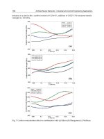
Figure 15 shows the comparison of the porposed method with incomplete observation, the
conventional actor-critic method and PID method for the angle,
θ
. In this figure, the
proposed method and PID method converge to zero smoothly, however the conventional
actor-critic method does not converge. The comparison of the proposed method with PID
control, the latter method converges quickly. These results are corresponding to Fig.16, i.e.
the torque of the PID method converges first, the next one is the proposed method, and the
conventional one does not converge.

-20
-10
0
10

20
0 2 4 6 8 10
Incomplete state observation using State-filter RL+SMC
actor-critic RL
PID

Fig. 16. Comparison of the porposed method with incomplete observation, the conventional
actor-critic method and PID method for the Torque,
q
T .


-0.1
-0.05
0
0.05
0.1
0.15
0.2
0 0.5 1 1.5 2 2.5 3 3.5 4
Angle [rad]
TIME
[
sec
]
Incomplete state observation using State-filter RL+SMC
Complete state observation RL+SMC
Incomplete state observation using Differencial RL+SMC

Fig. 17. The comparison of the porposed method among the case of the complete observation,

the case with the state variable filter, and with the difference method for the angle,
θ
.
A Robust Reinforcement Learning System Using Concept of
Sliding Mode Control for Unknown Nonlinear Dynamical System

211
Fig. 17 shows the comparison of the porposed method among the case of the complete
observation, the case with the state variable filter, and with the difference method for the
angle,
θ
. Among them, the incomplete state observation with the difference method is best
of three, especially, better than the complete observation. This reason can be explained by
Fig. 18. That is, the value of
s
of the case of the difference method is bigger than that of the
observation of the velocity angle, this causes that the input gain becomes bigger and the
convergence speed has been accelerated.

-0.4
-0.2
0
0.2
0.4
0.6
0.8
1
0 5 10 15 20
TIME
[

sec
]
Sliding using Velocity
Sliding using Differencial

Fig. 18. The values of the sliding variable
s
for using the velocity and the difference between
the angle and 1 sampling past angle.
5.4.4 Verification of the robust performance of each method
At first, as above mentioned, each controller was designed at
1.0 [kg]m =
in Eq. (21). Next
we examined the range of
m
in which the inverted pendulum control is success. Success is
defined as the case that if
/45≤
θπ
through the last 1[sec]. Results of the robust
performance for change of m are shown in Table 4. As to upper/lower limit of m for
success, the proposed method is better than the conventional actor-critic method not only
for gradually changing
m smaller from 1.0 to 0.001, but also for changing m bigger from 1.0
to 2.377. However, the best one is the conventional SMC method, next one is the PID control
method.
6. Conclusion
A robust reinforcement learning method using the concept of the sliding mode control was
mainly explained. Through the inverted pendulum control simulation, it was verified that
the robust reinforcement learning method using the concept of the sliding mode control has

good performance and robustness comparing with the conventional actor-critic method,
because of the making use of the ability of the SMC method.