Robust Control Theory and Applications Part 7 pot

Robust Controller Design: New Approaches in the Time and the Frequency Domains

227
11
0.5608 0.8553 0.5892 2.3740 0.7485
0.6698 1.3750 0.9909 1.3660 3.4440
3.1917 1.7971 2.5887 0.9461 9.6190
AB
−
⎡
⎤⎡ ⎤
⎢
⎥⎢ ⎥
=−− =
⎢
⎥⎢ ⎥
⎢
⎥⎢ ⎥
−−
⎣
⎦⎣ ⎦

22
0.6698 1.3750 0.9909 0.1562 0.1306
2.8963 1.5292 10.5160 0.4958 4.0379
3.5777 2.8389 1.9087 0.0306 0.8947
AB
−−
⎡
⎤⎡ ⎤
⎢

⎥⎢ ⎥
=− − =−
⎢
⎥⎢ ⎥
⎢
⎥⎢ ⎥
−−
⎣
⎦⎣ ⎦

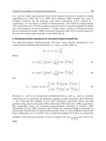
The uncertain system can be described by 4 vertices; corresponding maximal eigenvalues in
the vertices of open loop system are respectively: -4.0896 ± 2.1956i; -3.9243; 1.5014; -4.9595.
Notice, that the open loop uncertain system is unstable (positive eigenvalue in the third
vertex). The stabilizing optimal PD controller has been designed by solving matrix
inequality (25). Optimality is considered in the sense of guaranteed cost w.r.t. cost function
(23) with matrices
22 33
, 0.001 *RI Q I
×
×
=
= . The results summarized in Tab.2.1 indicate the
differences between results obtained for different choice of cost matrix S respective to a
derivative of x.


S
Controller matrices
F (proportional part)
F

d
(derivative part)
Max eigenvalues in
vertices

1e-6 *I
1.0567 0.5643
2.1825 1.4969
F
−−
⎡
⎤
=
⎢
⎥
−−
⎣
⎦

0.3126 0.2243
0.0967 0.0330
d
F
−−
⎡
⎤
=
⎢
⎥
−

⎣
⎦

-4.8644
-2.4074

-3.8368 ± 1.1165 i
-4.7436

0.1 *I
1.0724 0.5818
2.1941 1.4642
F
−−
⎡
⎤
=
⎢
⎥
−−
⎣
⎦

0.3227 0.2186
0.0969 0.0340
d
F
−−
⎡
⎤

=
⎢
⎥
−
⎣
⎦

-4.9546
-2.2211

-3.7823 ± 1.4723 i
-4.7751
Table 2.1 PD controllers from Example 2.1.
Example 2.2
Consider the uncertain system (1), (2) where
2.9800 0.9300 0 0.0340 0.0320
0.9900 0.2100 0.0350 0.0011 0
0001 0
0.3900 5.5550 0 1.8900 1.6000
AB
−−−
⎡⎤⎡⎤
⎢⎥⎢⎥
−− −
⎢⎥⎢⎥
==
⎢⎥⎢⎥
⎢⎥⎢⎥
−−−
⎣⎦⎣⎦

0010
0001
C
⎡
⎤
=
⎢
⎥
⎣
⎦

01.500 0
0000 0
0000 0
0000 0
AB
⎡
⎤⎡⎤
⎢
⎥⎢⎥
⎢
⎥⎢⎥
==
⎢
⎥⎢⎥
⎢
⎥⎢⎥
⎣
⎦⎣⎦

.
Robust Control, Theory and Applications

228
The results are summarized in Tab.2.2 for
44
1, 0.0005 *RQ I
×
=
= for various values of cost
function matrix S. As indicated in Tab.2.2, increasing values of S slow down the response as
assumed (max. eigenvalue of closed loop system is shifted to zero).

S q
max
Max. eigenvalue of closed loop system
1e-8 *I 1.1 -0.1890
0.1 *I 1.1 -0.1101
0.2 *I 1.1 -0.0863
0.29 *I 1.02 -0.0590
Table 2.2 Comparison of closed loop eigenvalues (Example 2.2) for various S.
3. Robust PID controller design in the frequency domain
In this section an original frequency domain robust control design methodology is presented
applicable for uncertain systems described by a set of transfer function matrices. A two-
stage as well as a direct design procedures were developed, both being based on the
Equivalent Subsystems Method - a Nyquist-based decentralized controller design method
for stability and guaranteed performance (Kozáková et al., 2009a;2009b), and stability
conditions for the M-
Δ
structure (Skogestad & Postlethwaite, 2005; Kozáková et al., 2009a,

2009b). Using the additive affine type uncertainty and related M
af
–Q structure stability
conditions, it is possible to relax conservatism of the M-
Δ
stability conditions (Kozáková &
Veselý, 2007).
3.1 Preliminaries and problem formulation
Consider a MIMO system described by a transfer function matrix ( )
mm
Gs R
×
∈ , and a
controller ( )
mm
Rs R
×
∈ in the standard feedback configuration (Fig. 1); w, u, y, e, d are
respectively vectors of reference, control, output, control error and disturbance of
compatible dimensions. Necessary and sufficient conditions for internal stability of the
closed-loop in Fig. 1 are given by the Generalized Nyquist Stability Theorem applied to the
closed-loop characteristic polynomial

det ( ) det[ ( )]Fs I Qs=+
(34)
where
() () ()Qs GsRs=
mm
R
×

∈
is the open-loop transfer function matrix.

w
e
y
u
d
R(s)
G(s)


Fig. 1. Standard feedback configuration
The following standard notation is used:
D - the standard Nyquist D-contour in the complex
plane;
Nyquist plot of ()gs - the image of the Nyquist contour under g(s); [,()]Nkgs - the
number of anticlockwise encirclements of the point
(k, j0) by the Nyquist plot of g(s).
Characteristic functions of ()Qs are the set of m algebraic functions ( ), 1, ,
i
qs i m
=
given as
Robust Controller Design: New Approaches in the Time and the Frequency Domains

229

det[ ( ) ( )] 0 1, ,
im

qsI Qs i m
−
==
(35)
Characteristic loci (CL) are the set of loci in the complex plane traced out by the
characteristic functions of
Q(s), sD
∀
∈ . The closed-loop characteristic polynomial (34)
expressed in terms of characteristic functions of
()Qs reads as follows

1
det ( ) det[ ( )] [1 ( )]
m
i
i
Fs I Qs q s
=
=+=+
∏
(36)
Theorem 3.1 (Generalized Nyquist Stability Theorem)
The closed-loop system in Fig. 1 is stable if and only if

1
a. det ( ) 0
b. [0,det ( )] {0,[1 ( )]}
m
i

q
i
Fs s D
NFsN qsn
=
≠∀∈
=
+=
∑
(37)
where
() ( ())Fs I Qs=+ and n
q
is the number of unstable poles of Q(s).
Let the uncertain plant be given as a set
Π
of N transfer function matrices

{ ( )}, 1,2, ,
k
Gs k N
Π
==
where
{
}
() ()
kk
ij
mm

Gs Gs
×
=
(38)

The simplest uncertainty model is the unstructured uncertainty, i.e. a full complex
perturbation matrix with the same dimensions as the plant. The set of unstructured
perturbations
D
U
is defined as follows

max max
: { ( ) : [ ( )] ( ), ( ) max [ ( )]}
U
k
DEj Ej Ej
ω
σωωω σω
=≤=
(39)

where ()
ω
 is a scalar weight function on the norm-bounded perturbation
()
mm
sR
Δ
×

∈ ,
max
[( )] 1j
σ
Δω
≤ over given frequency range,
max
()
σ
⋅
is the maximum singular value of (.),
i.e.


() ()()Ej j
ω
ωΔ ω
= 
(40)

For unstructured uncertainty, the set
Π
can be generated by either additive (E
a
),
multiplicative input (
E
i
) or output (E
o

) uncertainties, or their inverse counterparts (E
ia
, E
ii
,
E
io
), the latter used for uncertainty associated with plant poles located in the closed right
half-plane (Skogestad & Postlethwaite, 2005).
Denote
()Gs any member of a set of possible plants ,,,,,,
k
k a i o ia ii io
Π
=
;
0
()Gsthe nominal
model used to design the controller, and
()
k
ω
 the scalar weight on a normalized
perturbation. Individual uncertainty forms generate the following related sets
k
Π
:
Additive uncertainty:

0
max 0
:{():() () (),() ()()}
( ) max [ ( ) ( )], 1,2, ,
aaaa
k
a
k
Gs Gs G s E s E
jj
Gj Gj k N
Π
ωωΔω
ωσ ωω
==+ ≤
=−=

…
(41)
Robust Control, Theory and Applications

230
Multiplicative input uncertainty:

0
1
max 0 0
: { ( ) : ( ) ( )[ ( )], ( ) ( ) ( )}
( ) max { ( )[ ( ) ( )]}, 1,2, ,
iiii

k
i
k
Gs Gs G s I E s E
jjj
G
j
G
j
G
j
kN
Π
ωωΔω
ωσ ωωω
−
=
=+ ≤
=−=

…
(42)
Multiplicative output uncertainty:

00
1
max 0 0
:{():()[ ()](),() ()()}
() max {[ ( ) ( )] ( )}, 1,2, ,
ooo

k
o
k
Gs Gs I E s G s E
jjj
G
j
G
j
G
j
kN
Π
ωωΔω
ωσ ωωω
−
=
=+ ≤
=− =

…
(43)
Inverse additive uncertainty

1
00
11
max 0
:{():() ()[ ()()], () ()()}
( ) max {[ ( )] [ ( )] }, 1,2, ,

ia ia ia ia
k
ia
k
Gs Gs G s I E sG
j
E
jj
Gj Gj k N
ΠωωωΔω
ωσ ω ω
−
−−
==− ≤
=−=

…
(44)
Inverse multiplicative input uncertainty

1
0
1
max 0
: { (): () ()[ ()] , ( ) ( ) ( )}
( ) max { [ ( )] [ ( )]}, 1,2, ,
ii ii ii ii
k
ii
k

Gs Gs G s I E s E j j
IGj Gj k N
Π
ωωΔω
ωσ ω ω
−
−
==− ≤
=− =

…
(45)
Inverse multiplicative output uncertainty:

1
0
1
max 0
:{():()[ ()] (), () ()()}
( ) max { [ ( )][ ( )] }, 1,2, ,
io io io io
k
io
k
Gs Gs I E s G s E j j
IGj Gj k N
Π
ωωΔω
ωσ ωω
−

−
==− ≤
=− =

…
(46)
Standard feedback configuration with uncertain plant modelled using any above
unstructured uncertainty form can be recast into the M
Δ
−
structure (for additive
perturbation Fig. 2) where M(s) is the nominal model and
(
)
mm
sR
Δ
×
∈
is the norm-bounded
complex perturbation.
If the nominal closed-loop system is stable then M(s) is stable and
()s
Δ
is a perturbation
which can destabilize the system. The following theorem establishes conditions on M(s) so
that it cannot be destabilized by
()s
Δ
(Skogestad & Postlethwaite, 2005).

u
Δ

M(s)
y
Δ

Δ(s)
w
e
y
-
u
D

y
D

G
0
(s)
R(s)

(s)

a
∇

Fig. 2. Standard feedback configuration with unstructured additive uncertainty (left) recast
into the M
Δ
− structure (right)
Theorem 3.2 (Robust stability for unstructured perturbations)
Assume that the nominal system M(s) is stable (nominal stability) and the perturbation
()s
Δ
is stable. Then the M
Δ
−
system in Fig. 2 is stable for all perturbations
()s
Δ
:
max
() 1
σΔ
≤ if and only if
Robust Controller Design: New Approaches in the Time and the Frequency Domains

231

max
[()]1,Mj
σ
ωω
<
∀ (47)
For individual uncertainty forms

() (), ,,, , ,
kk
M
s M s k aioiaiiio
=
= ; the corresponding
matrices
()
k
M
s are given below (disregarding the negative signs which do not affect
resulting robustness condition); commonly, the nominal model
0
()Gs
is obtained as a model
of mean parameter values.

1
0
() () ()[ () ()] () ()
aaa
M
ssRsIGsRs sMs
−
=+ = additive uncertainty (48)

1
00
() () ()[ () ()] () () ()
iii

M
ssRsIGsRsGssMs
−
=+ = multiplicative input uncertainty (49)

1
00
() () () ()[ () ()] () ()
ooo
M
ssGsRsIGsRs sMs
−
=+=
multiplicative output uncertainty (50)

1
00
() ()[ () ()] () () ()
ia ia ia
M
ssIGsRsGssMs
−
=+ = inverse additive uncertainty (51)

1
0
() ()[ () ()] () ()
ii ii ii
M
ssIRsGs sMs

−
=+ = inverse multiplicative input uncertainty (52)

1
0
() ()[ () ()] () ()
io io io
M
ssIGsRs sMs
−
=+ =
inverse multiplicative output uncertainty (53)
Conservatism of the robust stability conditions can be reduced by structuring the
unstructured additive perturbation by introducing the additive affine-type uncertainty ()
af
Es
that brings about new way of nominal system computation and robust stability conditions
modifiable for the decentralized controller design as (Kozáková & Veselý, 2007; 2008).

1
() ()
p
a
f
ii
i
Es Gs
q
=
=

∑
(54)
where
()
mm
i
Gs R
×
∈
, i=0,1, …, p are stable matrices, p is the number of uncertainties defining
2
p
polytope vertices that correspond to individual perturbed models; q
i
are polytope
parameters. The set
a
f
Π
generated by the additive affine-type uncertainty (E
af
) is

0 min max min max
1
:{():() () , (), , , 0}
p
af af af i i i i i i i
i
Gs Gs G s E E G sq q q q q q

Π
=
==+= ∈<>+=
∑
(55)
where
0
()Gs is the „afinne“ nominal model. Put into vector-matrix form, individual
perturbed plants (elements of the set
a
f
Π
) can be expressed as follows

1
01 0
()
() () [ ] () ()
()
qqp u
p
Gs
Gs G s I I G s QG s
Gs
⎡⎤
⎢⎥
=+ =+
⎢⎥
⎢⎥
⎣

⎦
…
(56)
where
1
()
[]
p
mm
p
T
qq
QI I R
×
×
=∈… ,
i
q
imm
IqI
×
=
,
()
1
() [ ]
m
p
m
T

up
Gs G G R
×
×
=∈… .
Standard feedback configuration with uncertain plant modelled using the additive affine
type uncertainty is shown in Fig. 3 (on the left); by analogy with previous cases, it can be
recast into the
af
M
Q
−
structure in Fig. 3 (on the right) where
Robust Control, Theory and Applications

232

11
00
()()
af u u
M
GRI GR G I RG R
−−
=+ =+ (57)

w
e
y
u

Q

y
Q

-
G
0
(s)
R(s)

G
u
(s)

Q

u
Q

M
af
(s)
y
Q

Q

Fig. 3. Standard feedback configuration with unstructured affine-type additive uncertainty
(left), recast into the M

af
-Q structure (right)
Similarly as for the M-
Δ
system, stability condition of the
af
M
Q
−
system is obtained as

max
()1
af
MQ
σ
<
(58)
Using singular value properties, the small gain theorem, and the assumptions that
0min maxii
qq q==and the nominal model M
af
(s)

is stable, (58) can further be modified to
yield the robust stability condition

max 0
() 1
af

Mqp
σ
<
(59)
The main aim of Section 3 of this chapter is to solve the next problem.
Problem 3.1
Consider an uncertain system with m subsystems given as a set of N transfer function
matrices obtained in N working points of plant operation, described by a nominal model
0
()Gsand any of the unstructured perturbations (41) – (46) or (55).
Let the nominal model
0
()Gs can be split into the diagonal part representing mathematical
models of decoupled subsystems, and the off-diagonal part representing interactions
between subsystems

0
() () ()
dm
Gs Gs G s=+
(60)
where

() { ()}
dimm
Gs diagGs
×
= , det ( ) 0
d
Gs s≠∀

0
() () ()
md
Gs Gs Gs=− (61)
A decentralized controller

() { ()}
imm
Rs diagR s
×
=
, det ( ) 0Rs s D
≠
∀∈ (62)
is to be designed with
()
i
Rs being transfer function of the i-th local controller. The designed
controller has to guarantee stability over the whole operating range of the plant specified by
either (41) – (46) or (55) (robust stability) and a specified performance of the nominal model
(nominal performance). To solve the above problem, a frequency domain robust
decentralized controller design technique has been developed (Kozáková & Veselý, 2009;
Kozáková et. al., 2009b); the core of it is the Equivalent Subsystems Method (ESM).
Robust Controller Design: New Approaches in the Time and the Frequency Domains

233
3.2 Decentralized controller design for performance: equivalent subsystems method
The Equivalent Subsystems Method (ESM) an original Nyquist-based DC design method for
stability and guaranteed performance of the full system. According to it, local controller
designs are performed independently for so-called equivalent subsystems that are actually

Nyquist plots of decoupled subsystems shaped by a selected characteristic locus of the
interactions matrix. Local controllers of equivalent subsystems independently tuned for
stability and specified feasible performance constitute the decentralized controller
guaranteeing specified performance of the full system. Unlike standard robust approaches,
the proposed technique considers full mean parameter value nominal model, thus reducing
conservatism of resulting robust stability conditions. In the context of robust decentralized
controller design, the Equivalent Subsystems Method (Kozáková et. al., 2009b) is applied to
design a decentralized controller for the nominal model G
0
(s) as depicted in Fig. 4.

w
e
u
y
+
+
-
G
0
(s)

G
d
(s)
G
m
(s)
R(s)
R

1
0 … 0
0 R
2
… 0
………………
0 0 … R
m
G
11
0 … 0
0 G
22
… 0
………………
0 0 … G
mm

0 G
12
…G
1m
G
21
0

… G
2m
……………….…
G

m1
G
m2
… 0


Fig. 4. Standard feedback loop under decentralized controller
The key idea behind the method is factorisation of the closed-loop characteristic polynomial
detF(s) in terms of the split nominal system (60) under the decentralized controller (62)
(existence of
1
()Rs
−
is implied by the assumption (62) that det ( ) 0Rs
≠
)

{
}
1
det () det [ () ()] () det[ () () ()]det ()
dm dm
Fs IGsGsRs RsGsGs Rs
−
=+ + = ++ (63)
Denote

1
1
() () () () () ()

dm m
Fs R s Gs Gs Ps Gs
−
=++=+ (64)
where

1
() () ()
d
Ps R s G s
−
=+ (65)
is a diagonal matrix
() { ()}
imm
Ps diagp s
×
=
. Considering (63) and (64), the stability condition
(37b) in Theorem 3.1 modifies as follows
{0, det[ ( ) ( )]} [0, det ( )]
m
q
NPsGsNRsn
+
+= (66)
and a simple manipulation of (65) yields
Robust Control, Theory and Applications

234

()[ () ()] () () 0
eq
d
IRsGs Ps IRsGs
+
−=+ = (67)
where

( ) { ( )} { ( ) ( )} 1, ,
eq eq
mm i i mm
i
G s diag G s diag G s p s i m
××
==−=…
(68)
is a diagonal matrix of equivalent subsystems
()
eq
i
Gs; on subsystems level, (67) yields m
equivalent characteristic polynomials

() 1 () () 1,2, ,
eq eq
i
ii
CLCP s R s G s i m=+ = (69)
Hence, by specifying P(s) it is possible to affect performance of individual subsystems
(including stability) through

1
()Rs
−
. In the context of the independent design philosophy,
design parameters
(), 1,2, ,
i
p
si m= … represent constraints for individual designs. General
stability conditions for this case are given in Corollary 3.1.
Corollary 3.1 (Kozáková & Veselý, 2009)
The closed-loop in Fig. 4 comprising the system (60) and the decentralized controller (62) is
stable if and only if
1.
there exists a diagonal matrix
1, ,
() { ()}
ii m
Ps diagp s
=
=
such that all equivalent
subsystems (68) can be stabilized by their related local controllers R
i
(s), i.e. all
equivalent characteristic polynomials
() 1 () ()
eq eq
i
ii

CLCP s R s G s=+ , 1,2, ,im
=
have
roots with
Re{ } 0s
<
;
2.
the following two conditions are met sD
∀
∈ :

a. det[ () ()] 0
b. [0,det ( )]
m
q
Ps G s
NFsn
+
≠
=
(70)
where
(
)
det ( ) det ( ) ( )Fs I GsRs=+
and
q
n is the number of open loop poles with Re{ } 0s > .
In general,

()
i
p
s are to be transfer functions, fulfilling conditions of Corollary 3.1, and the
stability condition resulting form the small gain theory; according to it if both P
-1
(s) and
G
m
(s) are stable, the necessary and sufficient closed-loop stability condition is

1
() () 1
m
Ps G s
−
<
or
min max
[()] [ ()]
m
Ps G s
σσ
> (71)
To provide closed-loop stability of the full system under a decentralized controller,
(), 1,2, ,
i
p
si m= … are to be chosen so as to appropriately cope with the interactions ()
m

Gs.
A special choice of P(s) is addressed in (Kozáková et al.2009a;b): if considering characteristic
functions
()
i
gsof G
m
(s) defined according to (35) for 1, ,im= , and choosing P(s) to be
diagonal with identical entries equal to any selected characteristic function g
k
(s) of [-G
m
(s)],
where
{1, , }km∈ is fixed, i.e.

() ()
k
Ps g sI=− , {1, , }km∈ is fixed (72)
then substituting (72) in (70a) and violating the well-posedness condition yields

1
det[ () ()] [ () ()] 0
m
mki
i
Ps G s g s g s
=
+=−+=
∏

sD
∀
∈ (73)
Robust Controller Design: New Approaches in the Time and the Frequency Domains

235
In such a case the full closed-loop system is at the limit of instability with equivalent
subsystems generated by the selected
()
k
gs according to

() () () 1,2, ,
eq
ik
ik
Gs Gs
g
si m=+ =
, sD
∀
∈ (74)

Similarly, if choosing () ()
k
Ps g s I
α
α
−
=− − , 0

m
α
α
≤
≤ where
m
α
denotes the maximum
feasible degree of stability for the given plant under the decentralized controller
()Rs
, then

1
1
det() [()()]0
m
ki
i
Fs g s gs
ααα
=
−
=−−+ −=
∏
sD
∀
∈ (75)
Hence, the closed-loop system is stable and has just poles with
Re{ }s
α

≤
− , i.e. its degree of
stability is
α
. Pertinent equivalent subsystems are generated according to

()()() 1,2, ,
eq
ik
ik
Gs Gs gs i m
ααα
−= −+ − = (76)
To guarantee stability, the following additional condition has to be satisfied simultaneously

1
11
det [ ( ) ( )] ( ) 0
mm
kk i ik
ii
Fgsgsrs
α
==
=
−−+ = ≠
∏∏
sD
∀
∈ (77)

Simply put, by suitably choosing :
α
0
m
α
α
≤
≤ to generate ()Ps
α
−
it is possible to
guarantee performance under the decentralized controller in terms of the degree of
stability
α
. Lemma 3.1 provides necessary and sufficient stability conditions for the closed-
loop in Fig. 4 and conditions for guaranteed performance in terms of the degree of stability.
Definition 3.1 (Proper characteristic locus)
The characteristic locus ()
k
gs
α
−
of ()
m
Gs
α
−
, where fixed {1, , }km
∈
and 0

α
> , is called
proper characteristic locus if it satisfies conditions (73), (75) and (77). The set of all proper
characteristic loci of a plant is denoted
S
Ρ
.
Lemma 3.1
The closed-loop in Fig. 4 comprising the system (60) and the decentralized controller (62) is
stable if and only if the following conditions are satisfied
sD
∀
∈ , 0
α
≥ and
fixed
{1, , }km∈ :
1.
()
kS
gs P
α
−∈
2.
all equivalent characteristic polynomials (69) have roots with Res
α
≤
− ;
3.

[0,det ( )]
q
NFs n
α
α
−=

where
() ()()Fs I Gs Rs
α
αα
−=+ − −
;
q
n
α
is the number of open loop poles with
Re{ }s
α
>−
.
Lemma 3.1 shows that local controllers independently tuned for stability and a specified
(feasible) degree of stability of equivalent subsystems constitute the decentralized controller
guaranteeing the same degree of stability for the full system. The design technique resulting
from Corollary 3.1 enables to design local controllers of equivalent subsystems using any
SISO frequency-domain design method, e.g. the Neymark D-partition method (Kozáková et
al. 2009b), standard Bode diagram design etc. If considering other performance measures in
the ESM, the design proceeds according to Corollary 3.1 with
P(s) and
() () (), 1,2, ,

eq
ik
ik
Gs Gs gsi m=+ = generated according to (72) and (74), respectively.
Robust Control, Theory and Applications

236
According to the latest results, guaranteed performance in terms of maximum overshoot is
achieved by applying Bode diagram design for specified phase margin in equivalent
subsystems. This approach is addressed in the next subsection.
3.3 Robust decentralized controller design
The presented frequency domain robust decentralized controller design technique is
applicable for uncertain systems described as a set of transfer function matrices. The basic
steps are:
1.
Modelling the uncertain system
This step includes choice of the nominal model and modelling uncertainty using any
unstructured uncertainty (41)-(46) or (55). The nominal model can be calculated either as the
mean value parameter model (Skogestad & Postlethwaite, 2005), or the “affine” model,
obtained within the procedure for calculating the affine-type additive uncertainty
(Kozáková & Veselý, 2007; 2008). Unlike the standard robust approach to decentralized
control design which considers diagonal model as the nominal one (interactions are
included in the uncertainty), the ESM method applied in the design for nominal
performance allows to consider the
full nominal model.
2.
Guaranteeing nominal stability and performance
The ESM method is used to design a decentralized controller (62) guaranteeing stability and
specified performance of the nominal model (nominal stability, nominal performance).
3.

Guaranteeing robust stability
In addition to nominal performance, the decentralized controller has to guarantee closed-
loop stability over the whole operating range of the plant specified by the chosen
uncertainty description (robust stability). Robust stability is examined by means of the
M-
Δ

stability condition (47) or the
M
af-
-Q stability condition (59) in case of the affine type additive
uncertainty (55).
Corollary 3.2 (Robust stability conditions under DC)
The closed-loop in Fig. 3 comprising the uncertain system given as a set of transfer function
matrices and described by any type of unstructured uncertainty (41) – (46) or (55) with
nominal model fulfilling (60), and the decentralized controller (62) is stable over the
pertinent uncertainty region if any of the following conditions hold
1.
for any (41)–(46), conditions of Corollary 3.1 and (47) are simultaneously satisfied where
() (), ,,, , ,
kk
M
s M s k aioiaiiio== and M
k
given by (48)-(53) respectively.
2.
for (55), conditions of Corollary 3.1 and (59) are simultaneously satisfied.
Based on Corollary 3.2, two approaches to the robust decentralized control design have been
developed: the two-stage and the direct approaches.
1.

The two stage robust decentralized controller design approach based on the M-
Δ
structure stability
conditions
(Kozáková & Veselý, 2008;, Kozáková & Veselý, 2009; Kozáková et al. 2009a).
In the first stage, the decentralized controller for the nominal system is designed using ESM,
afterwards, fulfilment of the
M-
Δ
or M
af
-Q stability conditions (47) or (59), respectively is
examined; if satisfied, the design procedure stops, otherwise the second stage follows: either
controller parameters are additionally modified to satisfy robust stability conditions in the
tightest possible way (Kozáková et al. 2009a), or the redesign is carried out with modified
performance requirements (Kozáková & Veselý, 2009).
Robust Controller Design: New Approaches in the Time and the Frequency Domains

237
2. Direct decentralized controller design for robust stability and nominal performance
By direct integration of the robust stability condition (47) or (59) in the ESM, local controllers
of equivalent subsystems are designed with regard to robust stability. Performance
specification for the full system in terms of the maximum peak of the complementary
sensitivity
T
M
corresponding to maximum overshoot in individual equivalent subsystems
is translated into lower bounds for their phase margins according to (78) (Skogestad &
Postlethwaite, 2005)

11
2arcsin [ ]
2
TT
PM rad
MM
⎛⎞
≥≥
⎜⎟
⎝⎠
(78)
where PM is the phase margin, M
T
is the maximum peak of the complementary sensitivity

1
() () ()[ () ()]Ts GsRs I GsRs
−
=+
(79)
As for MIMO systems

max
()
T
M
T
σ
= (80)
the upper bound for M

T
can be obtained using the singular value properties in
manipulations of the M-
Δ
condition (47) considering (48)-(53), or the M
af
– Q condition (58)
considering (57) and (59). The following upper bounds
max 0
[( )]Tj
σ
ω
for the nominal
complementary sensitivity
1
00 0
() () ()[ () ()]Ts GsRsI GsRs
−
=+ have been derived:

min 0
max 0
[()]
[( )] ()
()
A
a
G
j
Tj L

σ
ω
σ
ωωω
ω
<
=∀

additive uncertainty (81)

max 0
1
[( )] (), ,,
()
K
k
Tj L k io
σ
ωωω
ω
<
==∀

multiplicative input/output uncertainty (82)

min 0
max 0
max
0
[()]

1
[( )] ()
[()]
AF
u
Gj
Tj L
Gj
qp
σ
ω
σ
ωωω
σω
<
=∀
additive affine-type uncertainty (83)
Using (80) and (78) the upper bounds for the complementary sensitivity of the nominal
system (81)-(83) can be directly implemented in the ESM due to the fact that performance
achieved in equivalent subsystems is simultaneously guaranteed for the full system. The
main benefit of this approach is the possibility to specify maximum overshoot in the full
system guaranteeing robust stability in terms of
max 0
()T
σ
, translate it into minimum phase
margin of equivalent subsystems and design local controllers independently for individual
single input – single output equivalent subsystems.
The design procedure is illustrated in the next subsection.
3.4 Example

Consider a laboratory plant consisting of two interconnected DC motors, where each
armature voltage (U
1
, U
2
) affects rotor speeds of both motors (ω
1
, ω
2
). The plant was
identified in three operating points, and is given as a set
123
{ ( ), ( ), ( )}GsGsGs
Π
= where
Robust Control, Theory and Applications

238
22
1
22
0.402 2.690 0.006 1.680
2.870 1.840 11.570 3.780
()
0.003 0.720 0.170 1.630
9.850 1.764 1.545 0.985
ss
ss s s
Gs
ss

ss ss
−
+−
⎡
⎤
⎢
⎥
++ + +
⎢
⎥
=
−−+
⎢
⎥
⎢
⎥
+
+++
⎣
⎦

22
2
22
0.342 2.290 0.005 1.510
2.070 1.840 10.570 3.780
()
0.003 0.580 0.160 1.530
8.850 1.764 1.045 0.985
ss

ss s s
Gs
ss
ss ss
−
+−
⎡
⎤
⎢
⎥
++ + +
⎢
⎥
=
−−+
⎢
⎥
⎢
⎥
+
+++
⎣
⎦

22
3
22
0.423 2.830 0.006 1.930
4.870 1.840 13.570 3.780
()

0.004 0.790 0.200 1.950
10.850 1.764 1.945 0.985
ss
ss s s
Gs
ss
ss ss
−
+−
⎡
⎤
⎢
⎥
++ + +
⎢
⎥
=
−−+
⎢
⎥
⎢
⎥
+
+++
⎣
⎦

In calculating the affine nominal model G
0
(s), all possible allocations of G

1
(s), G
2
(s), G
3
(s) into
the 2
2
= 4 polytope vertices were examined (24 combinations) yielding 24 affine nominal
model candidates and related transfer functions matrices G
4
(s) needed to complete the
description of the uncertainty region. The selected affine nominal model G
0
(s) is the one
guaranteeing the smallest additive uncertainty calculated according to (41):
22
0
22
-0.413 s +2.759 0.006 1.807
3.870 1.840 12.570 3.780
()
0.004 0.757 0.187 1.791
10.350 1.764 1.745 0.985
s
ss s s
Gs
ss
ss ss
−−

⎡
⎤
⎢
⎥
++ + +
⎢
⎥
=
−−+
⎢
⎥
⎢
⎥
++ ++
⎣
⎦

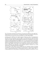
The upper bound
()
AF
L
ω
for T
0
(s) calculated according to (82) is plotted in Fig. 5. Its worst
(minimum value) min ( ) 1.556
TAF
ML
ω
ω

=
= corresponds to 37.48PM ≥

according to (78).

0
5 10 15 20 25 30
1.5
2
2.5
3
3.5
ω
[rad/s]


L
AF
(ω)

Fig. 5. Plot of L
AF
(
ω
) calculated according to (82)
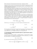
The Bode diagram design of local controllers for guaranteed PM was carried out for
equivalent subsystems generated according to (74) using characteristic locus g
1
(s) of the
matrix of interactions G

m
(s), i.e.
2
1
() () () 1,2
eq
i
i
Gs Gs gsi=+ =. Bode diagrams of equivalent
Robust Controller Design: New Approaches in the Time and the Frequency Domains

239
subsystems
11 21
(), ()
eq eq
GsGs are in Fig. 6. Applying the PI controller design from Bode diagram
for required phase margin
39PM =

has yielded the following local controllers
1
3.367 s +1.27
()Rs
s
=

2
1.803 0.491
()

s
Rs
s
+
=

Bode diagrams of compensated equivalent subsystems in Fig. 8 prove the achieved phase
margin. Robust stability was verified using the original M
af
-Q condition (59) with p=2 and
q
0
=1; as depicted in Fig. 8, the closed loop under the designed controller is robustly stable.


10

-3
10
-2
10
-1
10
0
10
1
10
2
-60
-40

-20
0
20
Magnitude [dB]

10

-3
10
-2
10
-1
10
0
10
1
10
2
-300
-200
-100
0
omega [rad/s]
Phasa [deg]


10
-3
10
-2

10
-1
10
0
10
1

10
2
-60
-40
-20
0
20
M
agn
i
tu
d
e
[dB]

10
-3
10
-2
10
-1
10
0

10
1

10
2
-300
-200
-100
0
omega [rad/s]
Ph
ase
[d
eg
]


Fig. 6. Bode diagrams of equivalent subsystems
11
()
eq
Gs(left),
21
()
eq
Gs(right)


10
-3

10

-2
10
-1
10
0
10
1
10
2
-50

0

50

100

ω
[rad/sec]
Magnitude [dB]
10
-3
10

-2
10
-1
10

0
10
1
10
2
-300

-200

-100

0

ω
[rad/sec]
phase [deg]

10
-3
10
-2
10
-1
10
0
10

1
10

2

-50
0
50
100
ω
[rad/sec]
Magnitude [dB]
10
-3
10
-2
10
-1
10
0
10

1
10

2

-300
-200
-100
0
ω
[rad/sec]

phase [deg]


Fig. 7. Bode diagrams of equivalent subsystems
11
()
eq
Gs(left),
21
()
eq
Gs(right) under designed
local controllers R
1
(s), R
2
(s), respectively.
Robust Control, Theory and Applications

240
0 5
10 15 20 25 30
0
0.1
0.2
0.3
0.4
0.5
0.6
0.7

ω
[rad/s]



Fig. 8. Verification of robust stability using condition (59) in the form
max
1
()
2
af
M
σ
<

4. Conclusion
The chapter reviews recent results on robust controller design for linear uncertain systems
applicable also for decentralized control design.
In the first part of the chapter the new robust PID controller design method based on LMI` is
proposed for uncertain linear system. The important feature of this PID design approach is
that the derivative term appears in such form that enables to consider the model
uncertainties. The guaranteed cost control is proposed with a new quadratic cost function
including the derivative term for state vector as a tool to influence the overshoot and
response rate.
In the second part of the chapter a novel frequency-domain approach to the decentralized
controller design for guaranteed performance is proposed. Its principle consists in including
plant interactions in individual subsystems through their characteristic functions, thus
yielding a diagonal system of equivalent subsystems. Local controllers of equivalent
subsystems independently tuned for specified performance constitute the decentralized
controller guaranteeing the same performance for the full system. The proposed approach

allows direct integration of robust stability condition in the design of local controllers of
equivalent subsystems.
Theoretical results are supported with results obtained by solving some examples.
5. Acknowledgment
This research work has been supported by the Scientific Grant Agency of the Ministry of
Education of the Slovak Republic, Grant No. 1/0544/09.
6. References
Blondel, V. & Tsitsiklis, J.N. (1997). NP-hardness of some linear control design problems.
SIAM J. Control Optim., Vol. 35, 2118-2127.
Boyd, S.; El Ghaoui, L.; Feron, E. & Balakrishnan, V. (1994). Linear matrix inequalities in system
and control theory, SIAM Studies in Applied Mathematics, Philadelphia.
Robust Controller Design: New Approaches in the Time and the Frequency Domains

241
Crusius, C.A.R. & Trofino, A. (1999). LMI Conditions for Output Feedback Control
Problems. IEEE Trans. Aut. Control, Vol. 44, 1053-1057.
de Oliveira, M.C.; Bernussou, J. & Geromel, J.C. (1999). A new discrete-time robust stability
condition. Systems and Control Letters, Vol. 37, 261-265.
de Oliveira, M.C.; Camino, J.F. & Skelton, R.E. (2000). A convexifying algorithm for the
design of structured linear controllers, Proc. 39
nd
IEEE CDC, pp. 2781-2786, Sydney,
Australia, 2000.
Ming Ge; Min-Sen Chiu & Qing-Guo Wang (2002). Robust PID controller design via LMI
approach. Journal of Process Control, Vol.12, 3-13.
Grman, Ľ. ; Rosinová, D. ; Kozáková, A. & Veselý, V. (2005). Robust stability conditions for
polytopic systems. International Journal of Systems Science, Vol. 36, No. 15, 961-973,
ISSN 1464-5319 (electronic) 0020-7721 (paper)
Gyurkovics, E. & Takacs, T. (2000). Stabilisation of discrete-time interconnected systems
under control constraints. IEE Proceedings - Control Theory and Applications, Vol. 147,

No. 2, 137-144
Han, J. & Skelton, R.E. (2003). An LMI optimization approach for structured linear
controllers, Proc. 42
nd
IEEE CDC, 5143-5148, Hawaii, USA, 2003
Henrion, D.; Arzelier, D. & Peaucelle, D. (2002). Positive polynomial matrices and improved
LMI robustness conditions. 15
th
IFAC World Congress, CD-ROM, Barcelona, Spain,
2002
Kozáková, A. & Veselý, V. (2007). Robust decentralized controller design for systems with
additive affine-type uncertainty. Int. J. of Innovative Computing, Information and
Control (IJICIC), Vol. 3, No. 5 (2007), 1109-1120, ISSN 1349-4198.
Kozáková, A. & Veselý, V. (2008). Robust MIMO PID controller design using additive
affine-type uncertainty. Journal of Electrical Engineering, Vol. 59, No.5 (2008), 241-
247, ISSN 1335 - 3632
Kozáková, A., Veselý, V. (2009). Design of robust decentralized controllers using the M-Δ
structure robust stability conditions. Int. Journal of Systems Science, Vol. 40, No.5
(2009), 497-505, ISSN 1464-5319 (electronic) 0020-7721 (paper).
Kozáková, A.; Veselý, V. & Osuský, J. (2009a). A new Nyquist-based technique for tuning
robust decentralized controllers, Kybernetika, Vol. 45, No.1 (2009), 63-83, ISSN 0023-
5954.
Kozáková, A.; Veselý,V. Osuský, J.(2009b). Decentralized Controllers Design for
Performance: Equivalent Subsystems Method, Proceedings of the European Control
Conference, ECC’09, 2295-2300, ISBN 978-963-311-369-1, Budapest, Hungary August
2009, EUCA Budapest.
Peaucelle, D.; Arzelier, D.; Bachelier, O. & Bernussou, J. (2000). A new robust D-stability
condition for real convex polytopic uncertainty. Systems and Control Letters, Vol. 40,
21-30
Rosinová, D.; Veselý, V. & Kučera, V. (2003). A necessary and sufficient condition for static

output feedback stabilizability of linear discrete-time systems. Kybernetika, Vol. 39,
447-459
Rosinová, D. & Veselý, V. (2003). Robust output feedback design of discrete-time systems –
linear matrix inequality methods. Proceedings 2
th
IFAC Conf. CSD’03 (CD-ROM),
Bratislava, Slovakia, 2003
Robust Control, Theory and Applications

242
Skelton, R.E.; Iwasaki, T. & Grigoriadis, K. (1998). A Unified Algebraic Approach to Linear
Control Design, Taylor and Francis, Ltd, London, UK
Skogestad, S. & Postlethwaite, I. (2005). Multivariable fedback control: analysis and design, John
Wiley & Sons Ltd., ISBN -13978-0-470-01167-6 (H/B), The Atrium, Southern Gate.
Chichester, West Sussex, UK
Veselý, V. (2003). Robust output feedback synthesis: LMI Approach, Proceedings 2
th
IFAC
Conference CSD’03 (CD-ROM), Bratislava, Slovakia, 2003
Zheng Feng; Qing-Guo Wang & Tong Heng Lee (2002). On the design of multivariable PID
controllers via LMI approach. Automatica, Vol. 38, 517-526

2. Discretized control system
The discretized control system in question is represented by a sampled-data (discrete-time)
feedback system as shown in Fig. 1. In the figure, G
(z) is the z-transform of continuous plant
G
(s) together with the zero-order hold, C(z) is the z-transform of the digital PID controller,
and
D

1
and D
2
are the discretizing units at the input and output sides of the nonlinear
element, respectively.
The relationship between e and u
†
= N
d
(e) is a stepwise nonlinear characteristic on an
integer-grid pattern. Figure 2 (a) shows an example of discretized sigmoid-type nonlinear
characteristic. For C-language expression, the input/output characteristic can be written as
e
†
= γ ∗(double)(int)(e/γ)
u = 0.4 ∗ e
†
+ 3.0 ∗atan(0.6 ∗e
†
) (1)
u
†
= γ ∗(double)(int)(u/γ),
where (int) and (double) denote the conversion into an integral number (a round-down
discretization) and the reconversion into a double-precision real number, respectively. Note
that even if the continuous characteristic is linear, the input/output characterisitc becomes
nonlinear on a grid pattern as shown in Fig. 2 (b), where the linear continuous characteristic
is chosen as u
= 0.85 ∗ e
†

.
In this study, a round-down discretization, which is usually executed on a computer, is
applied. Therefore, the relationship between e
†
and u
†
is indicated by small circles on the
stepwise nonlinear characteristic. Here, each signal e
†
, u
†
, ··· can be assigned to an integer
number as follows:
e
†
∈{···, −3γ, −2γ, −γ,0, γ,2γ,3γ, ···},
u
†
∈{···, −3γ, − 2γ, −γ,0, γ,2γ,3γ, ···},
where γ is the resolution of each variable. Without loss of generality, hereafter, it is assumed
that γ
= 1.0. That is, the variables e
†
, u
†
, ··· are defined by integers as follows:
e
†
, u
†

∈ Z, Z = {···−3, − 2, −1, 0, 1, 2, 3, ···}.
On the other hand, the time variable t is given as t
∈{0, h,2h,3h, ···}for the sampling period
h. When assuming h
= 1.0, the following expression can be defined:
t
∈ Z
+
, Z
+
= {0, 1, 2, 3, ···}.
Therefore, each signal e
†
(t), u
†
(t), ··· traces on a grid pattern that is composed of integers in
the time and controller variables space.
The discretized nonlinear characteristic
u
†
= N
d
(e
†
)=Ke
†
+ g(e
†
),0< K < ∞,(2)
as shown in Fig. 2(a) is partitioned into the following two sections:

|g(e
†
)|≤
¯
g
< ∞,(3)
for
|e
†
| < ε,and
|g(e
†
)|≤β |e
†
|,0≤ β ≤ K,(4)
244
Robust Control, Theory and Applications
(a) (b)
Fig. 2. Discretized nonlinear characteristics on a grid pattern.
for
|e
†
|≥ε. (In Fig. 2 (a) and (b), the threshold is chosen as ε = 2.0.)
Equation (3) represents a bounded nonlinear characteristic that exists in a finite region. On
the other hand, equation (4) represents a sectorial nonlinearity for which the equivalent linear
gain exists in a limited range. It can also be expressed as follows:
0
≤ g( e
†
)e

†
≤ βe
†2
≤ Ke
†2
.(5)
When considering the robust stability in a global sense, it is sufficient to consider the nonlinear
term (4) for
|e
†
|≥ε because the nonlinear term (3) can be treated as a disturbance signal. (In
the stability problem, a fluctuation or an offset of error is assumed to be allowable in
|e
†
| < ε.)
1 + qδ
g
∗
(·)
βqδ
❵
✲ ✲ ✲
❢
✲
✻
✲
ee
∗
v
∗

v
g
(e)
+
+
Fig. 3. Nonlinear subsystem g(e).
g
∗
(·)
W(β, q, z)
❣
❣
✲ ✲
❄
✛✛
✻
r

e
∗
v
∗
u

y

d

+
−

+
+
Fig. 4. Equivalent feedback system.
245
Robust Stabilization and Discretized PID Control
3. Equivalent discrete-time system
In this study, the following new sequences e
∗†
m
(k) and v
∗†
m
(k) are defined based on the above
consideration:
e
∗†
m
(k)=e
†
m
(k)+q ·
Δe
†
(k)
h
,(6)
v
∗†
m
(k)=v

†
m
(k) − βq ·
Δe
†
(k)
h
,(7)
where q is a non-negative number, e
†
m
(k) and v
†
m
(k) are neutral points of sequences e
†
(k) and
v
†
(k) ,
e
†
m
(k)=
e
†
(k)+e
†
(k −1)
2

,(8)
v
†
m
(k)=
v
†
(k)+v
†
(k −1)
2
,(9)
and Δe
†
(k) is the backward difference of sequence e
†
(k) ,thatis,
Δe
†
(k)=e
†
(k) −e
†
(k −1). (10)
The relationship between equations (6) and (7) with respect to the continuous values is shown
by the block diagram in Fig. 3. In this figure, δ is defined as
δ
(z) :=
2
h

·
1 − z
−1
1 + z
−1
. (11)
Thus, the loop transfer function from v
∗
to e
∗
can be given by W(β, q, z),asshowninFig.4,
where
W
(β, q, z)=
(
1 + qδ(z))G(z)C(z)
1 +(K + βqδ(z))G(z)C(z)
, (12)
and r

, d

are transformed exogenous inputs. Here, the variables such as v
∗
, u

and y

written
in Fig. 4 indicate the z-transformed ones.

In this study, the following assumption is provided on the basis of the relatively fast sampling
and the slow response of the controlled system.
[Assumption] The absolute value of the backward difference of sequence e
(k) does not
exceed γ, i.e.,
|Δe(k)| = |e(k) − e(k − 1)|≤γ. (13)
If condition (13) is satisfied, Δe
†
(k) is exactly ±γ or 0 because of the discretization. That is, the
absolute value of the backward difference can be given as
|Δe
†
(k)| = |e
†
(k) −e
†
(k −1)| = γ or 0. 
The assumption stated above will be satisfied by the following examples. The phase trace of
backward difference Δe
†
is shown in the figures.
246
Robust Control, Theory and Applications
Fig. 5. Nonlinear characteristics and discretized outputs.
4. Norm inequalities
In this section, some lemmas with respect to an 
2
norm of the sequences are presented. Here,
we define a new nonlinear function
f

(e) := g(e )+β e. (14)
When considering the discretized output of the nonlinear characteristic, v
†
= g(e
†
),the
following expression can be given:
f
(e
†
(k)) = v
†
(k)+βe
†
(k) . (15)
From inequality (4), it can be seen that the function (15) belongs to the first and third
quadrants. Figure 5 shows an example of the continuous nonlinear characteristics u
= N(e)
and f(e), the discretized outputs u
†
= N
d
(e
†
) and f(e
†
), and the sector (4) to be considered.
When considering the equivalent linear characteristic, the following inequality can be defined:
0
≤ ψ(k) :=

f (e
†
(k))
e
†
(k)
≤
2β. (16)
When this type of nonlinearity ψ
(k) is used, inequality (4) can be expressed as
v
†
(k)=g(e
†
(k)) = (ψ(k) − β)e
†
(k) . (17)
For the neutral points of e
†
(k) and v
†
(k) , the following expression is given from (15):
1
2
( f(e
†
(k)) + f (e
†
(k −1 ))) = v
†

m
(k)+βe
†
m
(k) . (18)
Moreover, equation (17) is rewritten as v
†
m
(k)=(ψ(k) − β)e
†
m
(k) .Since|e
†
m
(k)|≤|e
m
(k)|,the
following inequality is satisfied when a round-down discretization is executed:
|v
†
m
(k)|≤β|e
†
m
(k)|≤β|e
m
(k)|. (19)
247
Robust Stabilization and Discretized PID Control
Based on the above premise, the following norm conditions are examined

[Lemma-1] The following inequality holds for a positive integer p:
v
†
m
(k)
2,p
≤ βe
†
m
(k)
2,p
≤ βe
m
(k)
2,p
. (20)
Here,
·
2,p
denotes the Euclidean norm, which can be defined by
x(k)
2,p
:=

p
∑
k=1
x
2
(k)


1/2
.
(Proof) The proof is clear from inequality (19).

[Lemma-2] If the following inequality is satisfied with respect to the inner product of the
neutral points of (15) and the backward difference:
 v
†
m
(k)+βe
†
m
(k) , Δe
†
(k) 
p
≥ 0, (21)
the following inequality can be obtained:
v
∗†
m
(k)
2,p
≤ βe
∗†
m
(k)
2,p
(22)

for any q
≥ 0. Here, ·, ·
p
denotes the inner product, which is defined as
 x
1
(k) , x
2
(k) 
p
=
p
∑
k=1
x
1
(k)x
2
(k) .
(Proof) The following equation is obtained from (6) and (7):
β
2
e
∗†
m
(k)
2
2,p
−v
∗†

m
(k)
2
2,p
= β
2
e
†
m
(k)
2
2,p
−v
†
m
(k)
2
2,p
+
2βq
h
·v
†
m
(k)+βe
†
m
(k) , Δe
†
(k)

p
.
(23)
Thus, (22) is satisfied by using the left inequality of (20). Moreover, as for the input of g
∗
(·),
the following inequality can be obtained from (23) and the right inequality (20):
v
∗†
m
(k)
2,p
≤ βe
∗
m
(k)
2,p
. (24)

The left side of inequality (21) can be expressed as a sum of trapezoidal areas.
[Lemma-3] For any step p, the following equation is satisfied:
σ
(p ) :=  v
†
m
(k)+βe
†
m
(k) , Δe
†

(k) 
p
=
1
2
p
∑
k=1
( f(e
†
(k)) + f (e
†
(k −1)))Δe
†
(k) . (25)
(Proof) The proof is clear from (18).

In order to understand easily, an example of the sequences of continuous/discretized signals
and the sum of trapezoidal areas is depicted in Fig. 6. The curve e and the sequence of circles
e
†
show the input of the nonlinear element and its discretized signal. T he curve u and the
sequence of circles u
†
show the corresponding output of the nonlinear characteristic and its
discretized signal, respectively. As is shown in the figure, the sequences of circles e
†
and
u
†

trace on a grid pattern that is composed of integers. The sequence of circles v
†
shows
248
Robust Control, Theory and Applications
Fig. 6. Discretized input/output signals of a nonlinear element.
the discretized output of the nonlinear characteristic g
(·). The curve of shifted nonlinear
characteristic f
(e) and the sequence of circles f (e
†
) are also shown in the figure.
In general, the sum of trapezoidal areas holds the following property.
[Lemma-4] If inequality (13) is satisfied with respect to the discretization of the control
system, the sum of trapezoidal areas becomes non-negative for any p ,thatis,
σ
(p ) ≥ 0. (26)
(Proof) Since f
(e
†
(k)) belongs to the first and third quadrants, the area of each trapezoid
τ
(k) :=
1
2
( f(e
†
(k)) + f(e
†
(k −1)))Δe

†
(k) (27)
On the other hand, the trapezoidal area τ
(k) is non-positive when e(k) decreases (increases)
in the first (third) quadrant. Strictly speaking, when (e
(k) ≥ 0andΔe(k) ≥ 0) or
(e
(k) ≤ 0andΔe( k) ≤ 0), τ(k) is non-negative for any k. On the other hand, when
(e
(k) ≥ 0andΔe(k) ≤ 0) or (e(k) ≤ 0andΔe(k) ≥ 0), τ(k) is non-positive for any k. Here,
Δe
(k) ≥ 0 corresponds to Δe
†
(k)=γ or 0 (and Δe(k) ≤ 0 corresponds to Δe
†
(k)=−γ or 0)
for the discretized signal, when inequality (13) is satisfied.
The sum of trapezoidal area is given from (25) as:
σ
(p )=
p
∑
k=1
τ(k). (28)
Therefore, the following result is derived based on the above. The sum of trapezoidal areas
becomes non-negative, σ
(p ) ≥ 0, regardless of whether e(k) (and e
†
(k)) increases or decreases.
Since the discretized output traces the same points on the stepwise nonlinear characteristic,

the sum of trapezoidal areas is canceled when e
(k) (and e
†
(k) decreases (increases) from a
certain point
(e
†
(k) , f( e
†
(k))) in the first (third) quadrant. (Here, without loss of generality, the
response of discretized point
(e
†
(k) , f (e
†
(k))) is assumed to commence at the origin.) Thus,
the proof is concluded.

249
Robust Stabilization and Discretized PID Control
5. Robust stability in a global sense
By applying a small gain theorem to the loop transfer characteristic (12), the following robust
stability condition of the discretized nonlinear control system can be derived
[Theorem] If there exists a q
≥ 0 in which the sector parameter β with respect to nonlinear
term g
(·) satisfies the following inequality, the discrete-time control system with sector
nonlinearity (4) is robust stable in an

2

sense:
β
< β
0
= K · η( q
0
, ω
0
)=max
q
min
ω
K · η(q, ω), (29)
when the linearized system with nominal gain K is stable.
The η-function is written as follows:
η
(q, ω) :=
−
qΩ sin θ +

q
2
Ω
2
sin
2
θ + ρ
2
+ 2ρ cos θ + 1
ρ

,
∀ω ∈ [0, ω
c
], (30)
where Ω
(ω) is the distorted frequency of angular frequency ω and is given by
δ
(e
jωh
)=jΩ( ω)=j
2
h
tan

ωh
2

, j
=
√
−1 (31)
and ω
c
is a cut-off frequency. In addition, ρ(ω) and θ(ω) are the absolute value and the phase
angle of KG
(e
jωh
)C(e
jωh
), respectively.

(Proof) Based on the loop characteristic in Fig. 4, the following inequality can be given with
respect to z
= e
jωh
:
e
∗
m
(z)
2,p
≤ c
1
r

m
(z)
2,p
+ c
2
d

m
(z)
2,p
+ sup
z=1
|W(β, q, z)|·w
∗†
m
(z)

2,p
. (32)
Here, r

m
(z) and d

m
(z) denote the z-transformation for the neutral points of sequences r

(k)
and d

(k) , respectively. Moreover, c
1
and c
2
are positive constants.
By applying inequality (24), the following expression is obtained:

1
− β ·sup
z=1
|W(β, q, z)|

e
∗
m
(z)
2,p

≤ c
1
r

m
(z)
2,p
+ c
2
d

m
(z)
2,p
. (33)
Therefore, if the following inequality (i.e., the small gain theorem with respect to

2
gains) is
valid,
|W(β, q,e
jωh
)| =





(1 + jqΩ(ω))P(e
jωh

)C(e
jωh
)
1 +(K + jβqΩ(ω))P(e
jωh
)C(e
jωh
)





=





(1 + jqΩ(ω))ρ(ω)e
jθ(ω)
K +(K + jβqΩ(ω))ρ(ω)e
jθ(ω)





<
1

β
.
(34)
the sequences e
∗
m
(k) , e
m
(k) , e(k) and y (k) in the feedback system are restricted in finite values
when exogenous inputs r
(k) , d(k) are finite and p → ∞. (The definition of 
2
stable for
discrete-time systems was given in (10; 11).)
From the square of both sides of inequality (34),
β
2
ρ
2
(1 + q
2
Ω
2
) < (K + Kρ cos θ − βρqΩ sin θ)
2
+(Kρ sin θ + βρqΩ cos θ)
2
.
250
Robust Control, Theory and Applications

Fig. 7. An example of modified Nichols diagram (M = 1.4, c
q
= 0.0, 0.2, ···,4.0).
ρ
GP
2
GP
1
Q
2
M
p
θ
P
2
Thus, the following quadratic inequality can be obtained:
β
2
ρ
2
< −2βKρqΩ sin θ + K
2
(1 + ρ cos θ)
2
+ K
2
ρ
2
sin
2

θ. (35)
Consequently, as a solution of inequality (35),
β
<
−
KqΩ sin θ + K

q
2
Ω
2
sin
2
θ + ρ
2
+ 2ρ cos θ + 1
ρ
= Kη(q, ω). (36)

6. Modified Nichols diagram
In the previous papers,the inverse function was used instead of the η-function, i.e.,
ξ
(q, ω)=
1
η(q, ω)
.
Using the notation, inequality (29) can be rewritten as follows:
M
0
= ξ(q

0
, ω
0
)=min
q
max
ω
ξ(q, ω) <
K
β
. (37)
When q
= 0, the ξ-function can be expressed as:
ξ
(0, ω)=
ρ

ρ
2
+ 2ρ cos θ + 1
= |T(e
jωh
)|, (38)
where T
(z) is the complementary sensitivity function for the discrete-time system.
It is evident that the following curve on the gain-phase plane,
ξ
(0, ω)=M, (M :const.) (39)
251
Robust Stabilization and Discretized PID Control