Robust Control Theory and Applications Part 8 potx
Bạn đang xem bản rút gọn của tài liệu. Xem và tải ngay bản đầy đủ của tài liệu tại đây (3.29 MB, 40 trang )
Simple Robust Normalized PI Control for Controlled Objects with One-order Modelling Error
267
1
'( ) '( )
()
() ()
ss
s
ss
uvor
v
uv
ωωλ
ω
ωω
==−
=
(21)
Solutions of control parameters:
Solving these simultaneous equations, the following functions can be obtained:
(, )
(, , ) ( 1,2, , )
j
isj
p
Kgp j
s
ω fa
a
ω
α
=
=="
(22)
where
s
ω
is the stationary points vector.
Multiple solutions of
i
K
can be used to check for mistakes in calculation.
3.4 Example of a second-order system with one-order modelling error
In this section, an IP control system in continuous design for a second-order original
controlled object without one-order sensor and signal conditioner dynamics is assumed for
simplicity. The closed loop system with uncertain one-order modeling error is normalized
and obtained the stable region of the integral gain in the three tuning region classified by
the amplitude of P control parameter using Hurwits approach. Then, the safeness of the
only I tuning region and the risk of the large P tuning region are discussed. Moreover, the
analytic solutions of stationary points and double same integral gains are obtained using
the Stationary Points Investing on Fraction Equation approach for the gain curve of a
closed loop system.
Here, an
IP control system for a second-order controlled object without sensor dynamics is
assumed.
Closed-loop transfer function:
2
22
()
2
on
nn
K
Gs
ss
ω
ς
ωω
=
++
(23)
()
1
s
K
Hs
s
ε
=
+
(24)
2
22
1
() () ()
(1)(2 )
n
o
s
onn
Gs GsHs
KK s s s
ω
ε
ςω ω
==
++ +
(25)
,
n
n
s
s
ε
ωε
ω
=
(26)
432
(1 )( 1)
()
(2 1) ( 2 ) ( 1)
i
ii
Kpss
Ws
s
ssKpsK
ε
εςε ες
++
=
++++ +++
(27)
Stable conditions by Hurwits approach with four parameters:
a. In the case of a certain time constant
IPL&IPS Common Region:
Advances in Reinforcement Learning
268
23
0max[0,min[,,]]
i
Kkk
<
<∞
(28)
2
2
2( 2 1)
k
p
ς
εςε
ε
+
+
(29)
22 2
[{4 2 2 } (2 1)]p
ς
εςε ςε ςε
+
+−− +
(30)
22 22
22
3
2
[{4 2 2 } (2 1)]
8(21)
2
p
p
k
p
ς ε ςε ς ε ςε
ες ε ςε
ε
++−−+
+
+++
(31)
22
0422where p for
ς
εςε ςε
>++≤
IPL, IPS Separate Region:
The integral gain stability region is given by Eqs. (28)-(30).
2
22
2
22
22
(2 1)
0()
422
(2 1)
0()
422
422 0
p
PL
p
PS
for
+
<≤
++−
+
<<
++−
++−>
ςε
ςε ςε ς ε
ςε
ςε ςε ς ε
ςε ςε ς ε
(32)
It can be proven that
3
k
>0 in the IPS region, and
23
,0kk whenp→∞ →∞ →
(33)
IP0 Region:
2
2
2( 2 1)
00
(2 1)
i
Kwherep
ςε ςε
ςε
++
<
<=
+
(34)
The IP0 region is most safe because it has not zeros.
b. In the case of an uncertain positive time constant
IPL&IPS Common Region:
23
1
0max[0,min[,]] 0
p
i
Kkkwhenp
εεε
==
<
<>
(35)
'
3
(,, ) 0
p
where k p
ςε
=
22
422for
ς
ε
ς
ε
ς
ε
+
+<
(36)
2
4( 1)
min 1kwhen
p
ε
ς
ς
ε
+
=
=
(37)
IPL, IPS Separate Region:
This region is given by Eq. (32).
Simple Robust Normalized PI Control for Controlled Objects with One-order Modelling Error
269
IP0 Region:
2
,0 0.707
, 0.707
1
02(1) ,
2
p
i
K
εε ς
ες
ςς
ς
=<<
=+∞ >
<< −
(38)
2
( 0,0 0.707), 0
(1 2 )
p
when p
ς
ες
ς
=><<=
−
c. Robust loop gain margin
The following loop gain margin is obtained from eqs. (28) through (38) in the cases of certain
and uncertain parameters:
iUL
i
K
gm
K
(39)
where
iUL
K
is the upper limit of the stable loop gain
i
K
.
Stable conditions by Hurwits approach with three parameters:
The stability conditions will be shown in order to determine the risk of one order modelling
error
,
1
0()
2
i
K where p PL<≥
ς
(40)
21
00(0)
12 2
i
K where
p
P
p
ς
<< ≤<
−ς ς
(41)
Hurwits Stability is omitted because
h
is sufficiently small, although it can be checked using
the bilinear transform.
Robust loop gain margin:
(_ )
g
mPLregion
=
∞
(42)
It is risky to increase the loop gain in the
IPL region too much, even if the system does not
become unstable because a model order error may cause instability in the IPL region. In the
IPL region, the sensitivity of the disturbance from the output rises and the flat property of
the gain curve is sacrificed, even if the disturbance from the input can be isolated to the
output upon increasing the control gain.
Frequency transfer function:
222
0.5
22 2 2 2
{1 }
()[ ]
(2) {1 }
__ /
()1
+
−+−+
→=
=
ω
ω
ςω ω ω
ω
ω
ω
i
ii
s
s
Kp
Wj
KKp
solve local maximum minmum for
such that W j
(43)
When the evaluation function is considered to be two variable functions (
ω
and
i
K
) and the
stationary point is obtained, the system with the parameters does not satisfy the above
stability conditions.
Advances in Reinforcement Learning
270
Therefore, only the stationary points in the direction of
ω
will be obtained without
considering the evaluation function on
i
K
alone.
Stationary points and the integral gain:
Using the
Stationary Points Investing for Fraction Equation approach based on Lagrange’s
undecided multiplier approach with equality restriction, the following two loop gain
equations on
x are obtained. Both identities can be used to check for miscalculation.
22
1
0.5{ 2(2 1) 1}/{2 ( 1) }
i
K
xxxp
ςς
=+−++−
(44)
22
2
2
0.5{3 4(2 1) 1}/{2 (2 1) }
0
i
s
K
xxxp
where x
ςς
ω
=+−++−
=≥
(45)
Equating the right-hand sides of these equations, the third-order algebraic equation and the
solutions for semi-positive stationary points are obtained as follows:
2
2(2 1)(2 )
0, 1
p
xx
p
ςς
−−
=
=−
(46)
These points, which are called the first and second stationary points, call the first and second
tuning methods, respectively, which specify the points for gain 1.
4. Numerical results
In this section, the solutions of double same integral gain for a tuning region at the
stationary point of the gain curve of the closed system are shown and checked in some
parameter tables on normalized proportional gains and normalized damping coefficients.
Moreover, loop gain margins are shown in some parameter tables on uncertain time
constants of one-order modeling error and damping coefficients of original controlled
objects for some tuning regions contained with safest only I region.
1.08120.34800.7598-99-991.2
1.41161.30681.18921.04960.86120.8
-99
-99
0.6999
0.9
1.16471.04460.89320.64301.1
1.24571.13351.00000.81861.0
1.32711.21971.09630.94240.9
1.101.051.000.95
1.08120.34800.7598-99-991.2
1.41161.30681.18921.04960.86120.8
-99
-99
0.6999
0.9
1.16471.04460.89320.64301.1
1.24571.13351.00000.81861.0
1.32711.21971.09630.94240.9
1.101.051.000.95
Table 1.
p
ω
values for
ς
and
p
in IPL tuning by the first tuning method
1.18331.00420.83331.07911.01491.2
1.77501.50631.25001.00630.77500.8
1.1077
1.2272
0.6889
0.9
1.29091.09550.90910.73181.1
1.42001.20501.00000.80501.0
1.57781.33891.11110.89440.9
1.101.051.000.95
1.18331.00420.83331.07911.01491.2
1.77501.50631.25001.00630.77500.8
1.1077
1.2272
0.6889
0.9
1.29091.09550.90910.73181.1
1.42001.20501.00000.80501.0
1.57781.33891.11110.89440.9
1.101.051.000.95
Table 2.
12ii
KK=
values for
ς
and p in IPL tuning by the first tuning method
Simple Robust Normalized PI Control for Controlled Objects with One-order Modelling Error
271
Table 1 lists the stationary points for the first tuning method. Table 2 lists the integration
gains (
12ii
K
K=
) obtained by substituting Eq. (46) into Eqs. (44) and (45) for various
damping coefficients.
Table 3 lists the integration gains (
12ii
K
K=
) for the second tuning method.
1.01.2501.6672.505.001.7
0.55560.62500.71430.83331.01.3
2.50
1.667
1.250
0.9
0.83331.01.2501.6671.6
0.71430.83331.01.2501.5
0.62500.71430.83331.01.4
1.101.051.000.95
1.01.2501.6672.505.001.7
0.55560.62500.71430.83331.01.3
2.50
1.667
1.250
0.9
0.83331.01.2501.6671.6
0.71430.83331.01.2501.5
0.62500.71430.83331.01.4
1.101.051.000.95
Table 3.
12ii
K
K=
values for
ς
and
p
in IPL tuning by the second tuning method
Then, a table of loop gain margins (
1gm >
) generated by Eq. (39) using the stability limit
and the loop gain by the second tuning method on uncertain
ε
in a given region of
ε
for
each controlled
ς
by IPL (
p
=1.5) control is very useful for analysis of robustness. Then, the
unstable region, the unstable region, which does not become unstable even if the loop gain
becomes larger, and robust stable region in which uncertainty of the time constant, are
permitted in the region of
ε
.
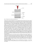
Figure 3 shows a reference step up-down response with unknown input disturbance in the
continuous region. The gain for the disturbance step of the IPL tuning is controlled to be
approximately 0.38 and the settling time is approximately 6 sec.
The robustness on indicial response for the damping coefficient change of ±0.1 is an
advantageous property. Considering
Zero Order Hold. with an imperfect dead-time
compensator using 1
st
-order Pade approximation, the overshoot in the reference step
response is larger than that in the original region or that in the continuous region.
00
( 1 0.1, 1.0, 1.5, 1.005, 1, 199.3, 0.0050674)
in
Kp s k
ςως
=± = = = = = =−
Fig. 3. Robustness of IPL tuning for damping coefficient change.
Then, Table 4 lists robust loop gain margins (
1gm >
) using the stability limit by Eq.(37) and
the loop gain by the second tuning method on uncertain
ε
in the region of
(0.1 10)
ε
≤≤
for
each controlled
ς
(>0.7) by IPL(
p
=1.5) control. The first gray row shows the area that is also
unstable
.
Advances in Reinforcement Learning
272
Table 5 does the same for each controlled
ς
(>0.4) by IPS(
p
=0.01). Table 6 does the same for
each controlled
ς
(>0.4) by IP0(
p
=0.0).
Table 4. Robust loop gain margins on uncertain
ε
in each region for each controlled
ς
at IPL
(
p
=1.5)
e
p
s/zita 0.4 0.5 0.6 0.7 0.8
0.1 1.189 1.832 2.599 3.484 4.483
0.6 1.066 1.524 2.021 2.548 3.098
1 1.097 1.492 1.899 2.312 2.729
2.1 1.254 1.556 1.839 2.106 2.362
10 1.717 1.832 1.924 2.003 2.073
Table 5. Robust loop gain margins on uncertain
ε
in each region for each controlled
ς
at IPS
(
p
=0.01)
eps/zita 0.3 0.4 0.5 0.6 0.7 0.8 0.9 1
0.1 0.6857 1.196 1.835 2.594 3.469 4.452 5.538 6.722
0.4 0.6556 1.087 1.592 2.156 2.771 3.427 4.118 4.84
0.5 0.6604 1.078 1.556 2.081 2.645 3.24 3.859 4.5
0.6 0.6696 1.075 1.531 2.025 2.547 3.092 3.655 4.231
1 0.7313 1.106 1.5 1.904 2.314 2.727 3.141 3.556
2.1 0.9402 1.264 1.563 1.843 2.109 2.362 2.606 2.843
10 1.5722 1.722 1.835 1.926 2.004 2.073 2.136 2.195
9999 1.9995 2 2 2 2 2 2 2
Table 6. Robust loop gain margins on uncertain
ε
in each region for each controlled
ς
at IP0
(
p
=0.0)
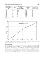
These table data with additional points were converted to the 3D mesh plot as following
Fig. 4. As IP0 and IPS with very small
p
are almost equivalent though the equations differ
quiet, the number of figures are reduced. It implies validity of both equations.
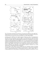
According to the line of worst loop gain margin as the parameter of attenuation in the
controlled objects which are described by gray label, this parametric stability margin (PSM)
(Bhattacharyya S. P., Chapellat H., and Keel L. H., 1994) is classified to 3 regions in IPS and
IP0 tuning regions and to 4 regions in IPL tuning regions as shown in Fig.5. We may call the
Simple Robust Normalized PI Control for Controlled Objects with One-order Modelling Error
273
larger attenuation region with more than 2 loop gain margin to the strong robust segment
region in which region uncertainty time constant of one-order modeling error is allowed in
the any region and some change of attenuation is also allowed.
(a)
p
=1.5 (b)
p
=1.0 (c)
p
=0.5 (d)
p
=0.01or 0
Fig. 4. Mesh plot of closed loop gain margin
Next, we call the larger attenuation region with more than 1>
γ
and less than 2 loop gain
margin to the weak robust segment region in which region uncertainty time constant of
one-order modeling error is only allowed in some region over some larger loop gain margin
and some larger change of attenuation is not allowed. The third and the forth segment is
almost unstable. Especially, notice that the joint of each segment is large bending so that the
sensitivity of uncertainty for loop gain margin is larger more than the imagination.
(a)
p
=1.5 (b)
p
=0.01 (c)
p
=0 (d)
p
=1.5, 1.0, 0.5, 0.01
Fig. 5. The various worst lines of loop gain margin in a parameter plane (certain&uncertain)
Moreover, the readers had to notice that the strong robust region and weak robust region
of IPL is shift to larger damping coefficient region than ones of IPS and IP0. Then, this is
also one of risk on IPL tuning region and change of tuning region from IP0 or IPS to IPL
region.
5. Conclusion
In this section, the way to convert this IP control tuning parameters to independent type PI
control is presented. Then, parameter tuning policy and the reason adopted the policy on the
controller are presented. The good and no good results, limitations and meanings in this
chapter are summarized. The closed loop gain curve obtained from the second order example
with one-order feedback modeling error implies the butter-worth filter model matching
method in higher order systems may be useful. The Hardy space norm with bounded
window was defined for I, and robust stability was discussed for MIMO system by an
expanssion of small gain theorem under a bounded condition of closed loop systems.
Advances in Reinforcement Learning
274
- We have obtained first an integral gain leading type of normalized IP controller to
facilitate the adjustment results of tuning parameters explaining in the later. The
controller is similar that conventional analog controllers are proportional gain type of PI
controller. It can be converted easily to independent type of PI controller as used in recent
computer controls by adding some converted gains. The policy of the parameter tuning is
to make the norm of the closed loop of frequency transfer function contained one-order
modeling error with uncertain time constant to become less than 1. The reason of selected
the policy is to be able to be similar to the conventional expansion of the small gain
theorem and to be possible in PI control. Then, the controller and uncertainty of the model
becomes very simple. Moreover, a simple approach for obtaining the solution is proposed
by optimization method with equality restriction using Lagrange’s undecided multiplier
approach for the closed loop frequency transfer function.
-
The stability of the closed loop transfer function was investigated using Hurwits
Criteria as the structure of coefficients were known though they contained uncertain
time constant.
-
The loop gain margin which was defined as the ratio of the upper stable limit of integral
gain and the nominal integral gain, was investigated in the parameter plane of damping
coefficient and uncertain time constant. Then, the robust controller is safe in a sense if
the robust stable region using the loop gain margin is the single connection and changes
continuously in the parameter plane even if the uncertain time constant changes larger
in a wide region of damping coefficient and even if the uncertain any adjustment is
done. Then, IP0 tuning region is most safe and IPL region is most risky.
-
Moreover, it is historically and newly good results that the worst loop gain margin as
each damping coefficient approaches to 2 in a larger region of damping coefficients.
-
The worst loop gain margin line in the uncertainty time constant and controlled objects
parameters plane had 3 or 4 segments and they were classified strong robust segment
region for more than 2 closed loop gain margin and weak robust segment region for
more than
γ > 1 and less than 2 loop gain margin. Moreover, the author was presented
also risk of IPL tuning region and the change of tuning region.
-
It was not good results that the analytical solution and the stable region were
complicated to obtain for higher order systems with higher order modeling error
though they were easy and primary. Then, it was unpractical.
6. Appendix
A. Example of a second-order system with lag time and one-order modelling error
In this section, for applying the robust PI control concept of this chapter to systems with
lag time, the systems with one-order model error are approximated using Pade
approximation and only the simple stability region of the integral gain is shown in the
special proportional tuning case for simplicity because to obtain the solution of integral
gain is difficult.
Here, a digital IP control system for a second-order controlled object with lag time L without
sensor dynamics is assumed. For simplicity, only special proportional gain case is shown.
Transfer functions:
2
22
(1 0.5 )
(1 0.5 )
()
1 ( 1)(0.5 1) 2
Ls
n
nn
K
Ls
Ke K Ls
Gs
Ts Ts Ls s s
ω
ς
ωω
−
−
−
== =
++ +++
(A.1)
Simple Robust Normalized PI Control for Controlled Objects with One-order Modelling Error
275
1
, 0.5 0.5 {( 0.5 ) /(0.5 )}
0.5
n
TL T L TL
TL
ως
== +
(A2)
()
1
s
K
Hs
s
ε
=
+
(A3)
Normalized operation:
The normalize operations as same as above mentioned are done as follows.
,
n
n
s
sLLω
ω
(A4)
2
(1 0.5 )
()
21
Ls
Gs
ssς
−
=
++
(A5)
n
εεω
(A6)
1
()
1
H
s
sε
=
+
(A7)
1
i
i
nn
K
Kpp
ωω
=
(A8)
111
() ( ) () ( )
iin
n
Cs K p Cs K p
ss
ω
ω
=+ = +
(A9)
Closed loop transfer function:
The closed loop transfer function is obtained using above normalization as follows;
2
2
43 2
1 (1 0.5 )
()
(21)
()
1 (1 0.5 )
1( )
(1)(21)
(1 )(1 0.5 )( 1)
(2 1) ( 2 0.5 ) (1 0.5 )
i
i
i
iiii
Ls
Kp
sss
Ws
Ls
Kp
ssss
Kps Lss
ss pLKsKpLKsK
ς
ες
ε
εςε ες
−
+
++
=
−
++
+++
+− +
=
++++− ++− +
(A.10)
43 222
0.5
(1 0.5 )( 1)
()
(2 1) ( 2 0.5 )
i
ii
if p L then
KLss
Ws
ss LKssK
ε
εςε ες
=
−+
=
++++− ++
(A11)
432
0
(1 0.5 )( 1)
()
(2 1) ( 2 ) (1 0.5 )
i
ii
if p then
KLss
Ws
s
ssLKsK
ε
εςε ες
=
−+
=
+
+++ +− +
(A.12)
Advances in Reinforcement Learning
276
Stability analysis by Hurwits Approach
1.
21
0.5 , 0 min{ , }, 0, 0
0.5 (0.5 )
i
pLK
pL L p
ε
ς
ςε
+
<<< >>
−
22 2
{(2 1)(2 0.5 ) } (2 1) 0.5
ii
LK K when p L
ςε ς ε ε ςε
++− −> + =
(A13)
2
22
2( 2 1)
0.5
(2 1){(2 1) 0.5 }
i
K
when p L
L
ς
εςε
ςε ςε
+
+
>=
+++
(A14)
k
3
< k
2
then
2
22 22
22(21)
0min{, } 0.5
0.5 (2 1){(2 1) 0.5 }
i
Kwhen
p
L
LL
+++
<< =
+++
ες ςε ςε
ςε ςε
(A15)
In continuous region with one order modelling error,
22
2
00.5
(1 0.5 )
i
K
when p L
L
ς
<< =
+
(A16)
Analytical solution of Ki for flat gain curve using Stationary Points Investing for Fraction
Equation approach is complicated to obtain, then it is remained for reader’s theme.
In the future, another approach will be developed for safe and simple robust control.
B. Simple soft M/A station
In this section, a configuration of simple soft M/A station and the feedback control system
with the station is shown for a simple safe interlock avoiding dangerous large overshoot.
B.1 Function and configuration of simple soft M/A station
This appendix describes a simple interlock plan for an simple soft M/A station that has a
parameter-identification mode (manual mode) and a control mode (automatic mode).
The simple soft M/A station is switched from automatic operation mode to manual
operation mode for safety when it is used to switch the identification mode and the control
mode and when the value of Pv exceeds the prescribed range. This serves to protect the
plant; for example, in the former case, it operates when the integrator of the PID controller
varies erratically and the control system malfunctions. In the latter case, it operates when
switching from P control with a large steady-state deviation with a high load to PI or PID
control, so that the liquid in the tank spillovers. Other dangerous situations are not
considered here because they do not fall under general basic control.
There have several attempts to arrange and classify the control logic by using a case base.
Therefore, the M/A interlock should be enhanced to improve safety and maintainability;
this has not yet been achieved for a simple M/A interlock plan (Fig. A1).
For safety reasons, automatic operation mode must not be used when changing into manual
operation mode by changing the one process value, even if the process value recovers to an
appropriate level for automatic operation.
Semiautomatic parameter identification and PID control are driven by case-based data for
memory of tuners, which have a nest structure for identification.
This case-based data memory method can be used for reusing information, and preserving
integrity and maintainability for semiautomatic identification and control. The semiautomatic
approach is adopted not only to make operation easier but also to enhance safety relative to
the fully automatic approach.
Simple Robust Normalized PI Control for Controlled Objects with One-order Modelling Error
277
Notation in computer control (Fig. B1, B3)
Pv : Process value
Av: Actual value
Cv : Control value
Mv : Manipulated value
Sp: Set point
A : Auto
M : Manual
T : Test
Pv
Mv at manual mode
Cv
Mv
Mv at auto mode
Switch
Conditions
On Pv
Conditions
On M/A
Switch
M
A
Integrated
Switching
Logic
Self-holding
Logic
S
W
I
T
C
H
T Pv’
Pv
Mv at manual mode
Cv
Mv
Mv at auto mode
Switch
Conditions
On Pv
Conditions
On M/A
Switch
M
A
Integrated
Switching
Logic
Self-holding
Logic
S
W
I
T
C
H
T Pv’
Fig. B1 A Configuration of Simple Soft M/A Station
B.2 Example of a SISO system
Fig. B2 shows the way of using M/A station in a configuration of a SISO control system.
Fig. B2 Configuration of a IP Control System with a M/A Station for a SISO Controlled Object
where the transfer function needed in Fig.B2 is as follows.
1.
Controlled Object:
()
1
Ls
K
Gs e
Ts
−
=
+
2.
Sensor & Signal Conditioner:
()
1
s
s
s
K
Gs
Ts
=
+
3.
Controller:
2
1
( ) 0.5 ( 0.5 )
i
Cs K L
s
=+
4.
Sensor Caribration Gain: 1/
s
K
5.
Normalized Gain before M/A Station: 1/ 0.5TL
6.
Normalized Gain after M/A Station: 1/K
Fig. B3 shows examples of simulated results for 2 kinds of switching mode when
Pv
becomes higher than a given threshold. (a) shows one to out of service and (b) does to
manual mode.
In former, Mv is down and Cv is almost hold. In latter, Mv is hold and Cv is down.
Advances in Reinforcement Learning
278
Auto Manual
Cv
Sp
Av
PvMv
Auto Manual
Cv
Sp
Av
PvMv
Mv Pv
Cv
Av
Auto Out of Service
Mv Pv
Cv
Av
(a) Switching example from auto mode to
out of service by Pv High
(b) Switching example from auto mode to
manual mode by Pv High
Fig. B3 Simulation results for 2 kinds of switching mode
C. New norm and expansion of small gain theorem
In this section, a new range restricted norm of Hardy space with window(Kohonen T., 1995)
w
H
∞
is defined for I, of which window is described to notation of norm with superscript w,
and a new expansion of small gain theorem based on closed loop system like general
w
H
∞
control problems and robust sensitivity analysis is shown for applying the robust PI
control concept of this chapter to MIMO systems.
The robust control was aims soft servo and requested internal stability for a closed loop
control system. Then, it was difficult to apply process control systems or hard servo systems
which was needed strong robust stability without deviation from the reference value in the
steady state like integral terms.
The method which sets the maximum value of closed loop gain curve to 1 and the results of
this numerical experiments indicated the above sections will imply the following new
expansion of small gain theorem which indicates the upper limit of Hardy space norm of a
forward element using the upper limit of all uncertain feedback elements for robust
stability.
For the purpose using unbounded functions in the all real domain on frequency like integral
term in the forward element, the domain of Hardy norm of the function concerned on
frequency is limited clearly to a section in a positive real one-order space so that the function
becomes bounded in the section.
Proposition
Assuming that feedback transfer function H(s) (with uncertainty) are stable and the
following inequality is holds,
1
() , 1Hs
∞
≤
γ≥
γ
(C-1)
Moreover , if the negative closed loop system as shown in Fig.C-1 is stable and the following
inequality holds,
()
() 1
1()()
Gs
Ws
GsHs
∞
∞
=
≤
+
(C-2)
Simple Robust Normalized PI Control for Controlled Objects with One-order Modelling Error
279
then the following inequality on the open loop transfer function is hold in a region of
frequency.
min max
1
()() , 1 [ , ]
1
w
Gj Hj for
∞
ωω≤ γ≥ ω∈ωω
γ−
(C-3)
In the same feedback system, G(s) holds the following inequality in a region of frequency.
min max
() , 1 [ , ]
1
w
Gj for
∞
γ
ω≤ γ≥ ω∈ω ω
γ−
(C-4)
()Gs
()Hs
+-
Fig. C-1 Configuration of a negative feed back system
(proof)
Using triangle inequality on separation of norms of summension and inequality on
separation of norms of product like Helder’s one under a region of frequency
min max
[,]ωω ,
as a domain of the norm of Hardy space with window, the following inequality on the
frequency transfer function of
()Gj
ω
is obtained from the assumption of the proposition.
()
() 1
1()()
Gj
Wj
Gj Hj
∞
∞
ω
ω
=≤
+ω ω
(C-5)
() 1 ()() 1 () ()
1
1()
()
wwww
w
w
Gj Gj Hj Gj Hj
Hj
Gj
∞
∞∞∞
∞
∞
ω≤+ ω ω≤+ ω ω
−ω≤
ω
(C-6)
1
() 1, 1
1
()
1
1()
w
w
w
if H j then
Gj
Hj
∞
∞
∞
ω≤≤γ≥
γ
γ
≥≥ω
γ−
−ω
(C-7)
Moreover, the following inequality on open loop frequency transfer function is shown.
1
() () ()()
1
ww w
Gj Hj Gj Hj
∞
∞∞
≥ω ω≥ωω
γ−
(C-8)
On the inequality of norm, the reverse proposition may be shown though the separation of
product of norms in the Hardy space with window are not clear. The sufficient conditions
on closed loop stability are not clear. They will remain reader’s theme in the future.
Advances in Reinforcement Learning
280
D. Parametric robust topics
In this section, the following three topics (Bhattacharyya S. P., Chapellat H., and Keel L. H., 1994.)
are introduced at first for parametric robust property in static one, dynamic one and stable one as
assumptions after linearizing a class of non-linear system to a quasi linear parametric variable
(QLPV) model by Taylar expansion using first order reminder term. (M.Katoh, 2010)
1.
Continuity for change of parameter
Boundary Crossing Theorem
1) fixed order polynomials P(λ,s)
2) continuous polynomials with respect to one parameter λ on a fixed interval I=[a,b].
If P(a,s) has all its roots in S, P(b,s) has at least one root in U, then there exists at least
one ρ in (a,b] such that:
a) P(ρ,s) has all roots in S U∂S
b) P(ρ,s) has at least one root in ∂S
P(a,s)
P(b,s)
P(ρ,s)
Fig. D-1 Image of boundary crossing theorem
2.
Convex for change of parameter
Segment Stable Lemma
Let define a segment using two stable polynomials as follows.
12
() () (1 ) ()
s
ss
λ
δλδ λδ
+−
12
12
[ (), ()] { (): [0,1]}
(), ()_ _ _ _deg _
___ __
ss s
where s s is polynomials of ree n
and stable with respect to S
λ
δδ δ λ
δδ
∈
(D-1)
Then, the followings are equivalent:
a) The segment
12
[(), ()]
s
s
δ
δ
is stable with respect to S
**
)()0, _ _ ; [0,1]b s for a ll s S
λ
δλ
≠∈∂∈
3.
Worst stability margin for change of parameter
Parametric stability margin (PSM) is defined as the worst case stability margin within
the parameter variation. It can be applied to a QLPV system of a class of non-linear
system. There are non-linear systems such as becoming worse stability margin than
linearized system although there are ones with better stability margin than it. There is a
case which is characterized by the one parameter m which describes the injection rate of
I/O, the interpolation rate of segment or degree of non-linearity.
E. Risk and Merit Analysis
Let show a summary and enhancing of the risk discussed before sections for safety in the following
table.
Simple Robust Normalized PI Control for Controlled Objects with One-order Modelling Error
281
Kinds Evaluation of influence Countermeasure
1) Disconnection of
feedback line
2) Overshoot over limit
value
1) Spill-over threshold
2) Attack to weak material
Auto change to manual
mode by M/A station
Auto shut down
Change of tuning region
from IPS to IPL by making
proportional gain to large
Grade down of stability
region from strong or weak
to weak or un-stability
Use IP0 and not use IPS
Not making proportional
gain to large in IPS tuning
region
Change of damping
coefficient or inverse of
time constant over weak
robust limit
Grade down of stability
region from strong or weak
to weak or un-stability
Change of tuning region
from IPL to IPS or IP0
Table E-1 Risk analysis for safety
It is important to reduce risk as above each one by adequate countermeasures after
understanding the property of and the influence for the controlled objects enough.
Next, let show a summary and enhancing of the merit and demerit discussed before sections for
robust control in the following table, too.
Kinds Merit Demerit
1) Steady state error is
vanishing as time by effect
of integral
1) It is important property
in process control and hard
servo area
It is dislike property in soft
servo and robot control
because of hardness for
disturbance
There is a strong robust
stability damping region in
which the closed loop gain
margin for any uncertainty
is over 2 and almost not
changing.
It is uniform safety for
some proportional gain
tuning region and changing
of damping coefficient.
For integral loop gain
tuning, it recommends the
simple limiting sensitivity
approach.
1) Because the region is
different by proportional
gain, there is a risk of grade
down by the gain tuning.
There is a weak robust
stability damping region in
which the worst closed loop
gain margin for any
uncertainty is over given
constant.
1) It can specify the grade
of robust stability for any
uncertainty
1) Because the region is
different by proportional
gain, there is a risk of grade
down by the gain tuning.
It is different safety for
some proportional gain
tuning region.
Table E-2 Merit analysis for control
It is important to apply to the best application area which the merit can be made and the
demerit can be controlled by the wisdom of everyone.
Advances in Reinforcement Learning
282
7. References
Bhattacharyya S. P., Chapellat H., and Keel L. H.(1994). Robust Control, The Parametric
Approach, Upper Saddle River NJ07458 in USA: Prentice Hall Inc.
Katoh M. and Hasegawa H., (1998). Tuning Methods of 2
nd
Order Servo by I-PD Control
Scheme, Proceedings of The 41st Joint Automatic Control Conference, pp. 111-112. (in
Japanese)
Katoh M.,(2003). An Integral Design of A Sampled and Continuous Robust Proper
Compensator, Proceedings of CCCT2003, (pdf000564), Vol. III, pp. 226-229.
Katoh M.,(2008). Simple Robust Normalized IP Control Design for Unknown Input
Disturbance, SICE Annual Conference 2008, August 20-22, The University Electro-
Communication, Japan, pp.2871-2876, No.:PR0001/08/0000-2871
Katoh M., (2009). Loop Gain Margin in Simple Robust Normalized IP Control for Uncertain
Parameter of One-Order Model Error, International Journal of Advanced Computer
Engineering, Vol.2, No.1, January-June, pp.25-31, ISSN:0974-5785, Serials
Publications, New Delhi (India)
Katoh M and Imura N., (2009). Double-agent Convoying Scenario Changeable by an
Emergent Trigger, Proceedings of the 4
th
International Conference on Autonomous
Robots and Agents, Feb 10-12, Wellington, New Zealand, pp.442-446
Katoh M. and Fujiwara A., (2010). Simple Robust Stability for PID Control System of an
Adjusted System with One-Changeable Parameter and Auto Tuning, International
Journal of Advanced Computer Engineering, Vol.3, No.1, ISSN:0974-5785, Serials
Publications, New Delhi (India)
Katoh M.,(2010). Static and Dynamic Robust Parameters and PI Control Tuning of TV-MITE
Model for Controlling the Liquid Level in a Single Tank”, TC01-2, SICE Annual
Conference 2010, 18/August TC01-3
Krajewski W., Lepschy A., and Viaro U.,(2004). Designing PI Controllers for Robust Stability
and Performance, Institute of Electric and Electronic Engineers Transactions on Control
System Technology, Vol. 12, No. 6, pp. 973- 983.
Kohonen T.,(1995, 1997). Self-Organizing Maps, Springer
Kojori H. A., Lavers J. D., and Dewan S. B.,(1993). A Critical Assessment of the Continuous-
System Approximate Methods for the Stability Analysis of a Sampled Data System,
Institute of Electric and Electronic Engineers Transactions on Power Electronics, Vol. 8,
No. 1, pp. 76-84.
Miyamoto S.,(1998). Design of PID Controllers Based on H
∞
-Loop Shaping Method and LMI
Optimization, Transactions of the Society of Instrument and Control Engineers, Vol. 34,
No. 7, pp. 653-659. (in Japanese)
Namba R., Yamamoto T., and Kaneda M., (1998). A Design Scheme of Discrete Robust PID
Control Systems and Its Application, Transactions on Electrical and Electronic
Engineering, Vol. 118-C, No. 3, pp. 320-325. (in Japanese)
Olbrot A. W. and Nikodem M.,(1994) . Robust Stabilization: Some Extensions of the Gain
Margin Maximization Problem, Institute of Electric and Electronic Engineers
Transactions on Automatic Control, Vol. 39, No. 3, pp. 652- 657.
Zbou K. with Doyle F. C. and Glover K.,(1996). Robust and Optimal Control, Prentice Hall Inc.
Zhau K. and Khargonekar P.P., (1988). An Algebraic Riccati Equation Approach to H
Optimization, Systems & Control Letters, 11, pp.85-91.
actuator effectiveness. FTCs dealing with actuator faults are relevant in practical applications
and have already been the subject of many publications. For instance, in (43), the case
of uncertain linear time-invariant models was studied. The authors treated the problem
of actuators stuck at unknown constant values at unknown time instants. The active FTC
approach they proposed was based on an output feedback adaptive method. Another active
FTC formulation was proposed in (46), where the authors studied the problem of loss
of actuator effectiveness in linear discrete-time models. The loss of control effectiveness
was estimated via an adaptive Kalman filter. The estimation was complemented by a fault
reconfiguration based on the LQG method. In (30), the authors proposed a multiple-controller
based FTC for linear uncertain models. They introduced an active FTC scheme that ensured
the stability of the system regardless of the decision of FDD.
However, as mentioned earlier and as presented for example in (50), the aforementioned
active schemes will incur a delay period during which the associate FDD component will have
to converge to a best estimate of the fault. During this time period of FDD response delay,
it is essential to control the system with a passive fault tolerant controller which is robust
against actuator faults so as to ensure at least the stability of the system, before switching to
another controller based on the estimated post-fault model, that ensures optimal post-fault
performance. In this context, we propose here passive FTC schemes against actuator loss
of effectiveness. The results presented here are based on the work of the author introduced
in (6; 8). We first consider linear FTC and present some results on passive FTC for loss of
effectiveness faults based on absolute stability theory. Next we present an extension of the
linear results to some nonlinear models and use passivity theory to write nonlinear fault
tolerant controllers. In this chapter several controllers are proposed for different problem
settings: a) Linear time invariant (LTI) certain plants, b) uncertain LTI plants, c) LTI models
with input saturations, d) nonlinear plants affine in the control with single input, e) general
nonlinear models with constant as well as time-varying faults and with input saturation. We
underline here that we focus in this chapter on the theoretical developments of the controllers,
readers interested in numerical applications should refer to (6; 8).
2. Preliminaries
Throughout this chapter we will use the L
2
norm denoted ||.||,i.e.forx ∈ R
n
we define
||x|| =
√
x
T
x. The notation L
f
h denotes the standard Lie derivative of a scalar function h(.)
along a vector function f(.). Let us introduce now some definitions from (40), that will be
frequently used in the sequel.
Definition 1 ((40), p.45): The solution x
(t, x
0
) of the system
˙
x = f (x), x ∈ R
n
, f locally
Lipschitz, is stable conditionally to Z,ifx
0
∈ Z and for each > 0thereexistsδ() > 0
such that
||
˜
x
0
− x
0
|| < δ and
˜
x
0
∈ Z ⇒||x(t,
˜
x
0
) − x(t, x
0
)|| < , ∀t ≥ 0.
If furthermore, there exist r
(x
0
) > 0, s.t. ||x(t,
˜
x
0
) − x(t, x
0
)|| ⇒ 0, ∀| |
˜
x
0
− x
0
|| <
r(x
0
) and
˜
x
0
∈ Z, the solution is asymptotically stable conditionally to Z.Ifr(x
0
) → ∞,
the stability is global.
Definition 2 ((40), p.48): Consider the system H :
˙
x
= f (x, u), y = h(x, u), x ∈ R
n
, u, y ∈ R
m
,
with zero inputs, i.e.
˙
x
= f (x,0), y = h(x,0) and let Z ⊂ R
n
be its largest positively invariant
set contained in
{x ∈ R
n
|y = h(x,0)=0}. We say that H is globally zero-state detectable
(GZSD) if x
= 0 is globally asymptotically stable conditionally to Z.IfZ = {0}, the system H
is zero-state observable (ZSO).
284
Robust Control, Theory and Applications
Definition 3 ((40), p.27): We say that H is dissipative in X ⊂ R
n
containing x = 0, if there exists
afunctionS
(x), S(0)=0suchthatforallx ∈ X
S
(x) ≥ 0 and S(x(T)) −S(x(0)) ≤
T
0
ω(u(t), y(t))dt,
for all u
∈ U ⊂ R
m
and all T > 0suchthatx(t) ∈ X, ∀ t ∈ [0, T].Wherethefunction
ω : R
m
× R
m
→ R called the supply rate, is locally integrable for every u ∈ U,i.e.
t
1
t
0
|ω(u(t), y(t))|dt < ∞, ∀ t
0
≤ t
1
. S is called the storage function. If the storage function is
differentiable the previous conditions writes as
˙
S
(x(t)) ≤ ω(u(t), y(t)).
The system H is said to be passive if it is dissipative with the supply rate w
(u, y)=u
T
y.
Definition 4 ((40), p.36): We say that H is output feedback passive (OFP(ρ)) if it is dissipative
with respect to ω
(u, y)=u
T
y − ρy
T
y for some ρ ∈ R.
We will also need the following definition to study the case of time-varying faults in Section
8.
Definition 5 (24): Afunction
x : [0, ∞) → R
n
is called a limiting solution of the system
˙
x =
f (t, x ), f a smooth vector function, with respect to an unbounded sequence t
n
in [0, ∞),ifthere
exist a compact κ
⊂ R
n
and a sequence {x
n
: [t
n
, ∞) → κ} of solutions of the system such
that the associated sequence
{
ˆ
x
n
:→ x
n
(t + t
n
)} converges uniformly to x on every compact
subset of
[0, ∞).
Also, throughout this paper it is said that a statement P
(t) holds almost everywhere(a.e.) if the
Lebesgue measure of the set
{t ∈ [0, ∞) |P(t) is false}is zero. We denote by df the differential
of the function f : R
n
→ R. We also mean by semiglobal stability of the equilibrium point
x
0
for the autonomous system
˙
x = f(x), x ∈ R
n
with f a smooth function, that for each
compact set K
⊂ R
n
containing x
0
, there exist a locally Lipschitz state feedback, such that x
0
is asymptotically stable, with a basin of attraction containing K ((44), Definition 3, p. 1445).
3. FTC for known LTI plants
First, let us consider linear systems of the form
˙
x
= Ax + Bαu,(1)
where, x
∈ R
n
, u ∈ R
m
are the state and input vector, respectively, and α ∈ R
m×m
is a diagonal
time variant fault matrix, with diagonal elements α
ii
(t), i = 1, , m s.t., 0 <
1
≤ α
ii
(t) ≤ 1.
The matrices A, B have appropriate dimensions and satisfy the following assumption.
Assumption(1):Thepair
(A, B) is controllable.
3.1 Problem statement
Find a state feedback controller u(x) such that the closed-loop controlled system (1) admits x = 0 as a
globally uniformly asymptotically (GUA) stable equilibrium point
∀α(t)(s.t.0<
1
≤ α
ii
(t) ≤ 1).
3.2 Problem solution
Hereafter, we will re-write the problem of stabilizing (1), for ∀α(t) s.t., 0 <
1
≤ α
ii
(t) ≤ 1, as
an absolute stability problem or Lure’s problem (2). Let us first recall the definition of sector
nonlinearities.
285
Passive Fault Tolerant Control
Definition 6 ((22), p. 232): A static function ψ : [0, ∞) ×R
m
→ R
m
, s.t. [ψ(t, y) −K
1
y]
T
[ψ(t, y) −
K
2
y] ≤ 0, ∀(t, y),withK = K
2
− K
1
= K
T
> 0, where K
1
= diag(k1
1
, ,k1
m
), K
2
=
diag(k2
1
, ,k2
m
),issaidtobelongtothesector[K
1
, K
2
].
We can now recall the definition of absolute stability or Lure’s problem.
Definition 7 (Absolute stability or Lure’s problem (22), p. 264): We assume a linear system of the
form
˙
x
= Ax + Bu
y
= Cx+ Du
u
= −ψ(t, y),
(2)
where, x
∈ R
n
, u ∈ R
m
, y ∈ R
m
, (A, B) controllable, (A, C) observable and ψ : [0, ∞) ×
R
m
→ R
m
is a static nonlinearity, piecewise continuous in t, locally Lipschitz in y and satisfies
a sector condition as defined above. Then, the system (2) is absolutely stable if the origin
is GUA stable for any nonlinearity in the given sector. It is absolutely stable within a finite
domain if the origin is uniformly asymptotically (UA) stable within a finite domain.
We can now introduce the idea used here, which is as follows:
Let us associate with the faulty system (1) a virtual output vector y
∈ R
m
˙
x
= Ax + Bαu
y
= Kx,
(3)
and let us write the controller as an output feedback
u
= −y.(4)
From (3) and (4), we can write the closed-loop system as
˙
x
= Ax + Bv
y
= Kx
v
= −α(t)y.
(5)
We have thus transformed the problem of stabilizing (1), for all bounded matrices α
(t),tothe
problem of stabilizing the system (5) for all α
(t). It is clear that the problem of GUA stabilizing
(5) is a Lure’s problem in (2), with the linear time varying stationarity ψ
(t, y)=α(t)y,and
where the ‘nonlinearities’ admit the sector bounds K
1
= diag(
1
, ,
1
), K
2
= I
m×m
.
Based on this formulation we can now solve the problem of passive fault tolerant control of
(1) by applying the absolute stability theory (26).
We can first write the following result:
Proposition 1: Under Assumption 1, the closed-loop of (1) with the static state feedback
u
= −Kx,(6)
where K is solution of the optimal problem
min
k
ij
(
∑
i=m
i
=1
∑
j=n
j
=1
k
2
ij
)
P
ˆ
A
(K)+
ˆ
A
T
(K)P (
ˆ
C
T
− P
ˆ
B)W
−1
((
ˆ
C
T
− P
ˆ
B)W
−1
)
T
−I
< 0
P
> 0
rank
⎡
⎢
⎢
⎢
⎣
K
KA
.
.
.
KA
n−1
⎤
⎥
⎥
⎥
⎦
= n,
(7)
286
Robust Control, Theory and Applications
for P = P
T
> 0, W =(
ˆ
D
+
ˆ
D
T
)
0.5
and {
ˆ
A(K),
ˆ
B(K),
ˆ
C(K),
ˆ
D(K)} is a minimal realization
of the transfer matrix
ˆ
G
=[I + K(sI − A)
−1
B][ I +
1
× I
m×m
K(sI − A)
−1
B]
−1
,(8)
admits the origin x
= 0 as GUA stable equilibrium point.
Proof: We saw that the problem of stabilizing (1) with a static state feedback u
= −Kx is
equivalent to the stabilization of (5). Studying the stability of (5) is a particular case of Lure’s
problem defined by (2), with the ‘nonlinearity’ function ψ
(t, y)=−α(t)y associated with
the sector bounds K
1
=
1
× I
m×m
, K
2
= I
m×m
(introduced in Definition 1). Then based on
Theorem 7.1, in ((22), p. 265), we can write that under Assumption1 and the constraint of
observability of the pair
(A, K), the origin x = 0 is GUA stable equilibrium point for (5), if the
matrix transfer function
ˆ
G
=[I + G(s)] [I +
1
× I
m×m
G(s )]
−1
,
where G
(s)=K(sI − A)
−1
B, is strictly positive real (SPR). Now, using the KYP lemma as
presented in (Lemma 6.3, (22), p. 240), we can write that a sufficient condition for the GUA
stability of x
= 0 along the solution of (1) with u = −Kx is the existence of P = P
T
> 0, L and
W, s.t.
P
ˆ
A
(K)+
ˆ
A
T
(K)P = −L
T
L − P, > 0
P
ˆ
B
(K)=
ˆ
C
T
(K) − L
T
W
W
T
W =
ˆ
D
(K)+
ˆ
D
T
(K),
(9)
where,
{
ˆ
A,
ˆ
B,
ˆ
C,
ˆ
D} is a minimal realization of
ˆ
G. Finally, adding to equation (9), the
observability condition of the pair
(A, K), we arrive at the condition
P
ˆ
A
(K)+
ˆ
A
T
(K)P = −L
T
L − P, > 0
P
ˆ
B
(K)=
ˆ
C
T
(K) − L
T
W
W
T
W =
ˆ
D
(K)+
ˆ
D
T
(K)
rank
⎡
⎢
⎢
⎢
⎣
K
KA
.
.
.
KA
n−1
⎤
⎥
⎥
⎥
⎦
= n.
(10)
Next, if we choose W
= W
T
we can write W =(
ˆ
D
+
ˆ
D
T
)
0.5
. The second equation in (10) leads
to L
T
=(
ˆ
C
T
− P
ˆ
B)W
−1
. Finally, from the first equation in (10), we arrive at the following
condition on P
P
ˆ
A
(K)+
ˆ
A
T
(K)P +(
ˆ
C
T
− P
ˆ
B)W
−1
((
ˆ
C
T
− P
ˆ
B)W
−1
)
T
< 0,
whichisinturnequivalenttotheLMI
P
ˆ
A
(K)+
ˆ
A
T
(K)P (
ˆ
C
T
− P
ˆ
B)W
−1
((
ˆ
C
T
− P
ˆ
B)W
−1
)
T
−I
< 0. (11)
Thus, to solve equation (10) we can solve the constrained optimal problem
287
Passive Fault Tolerant Control
min
k
ij
(
∑
i=m
i
=1
∑
j=n
j
=1
k
2
ij
)
P
ˆ
A
(K)+
ˆ
A
T
(K)P (
ˆ
C
T
− P
ˆ
B)W
−1
((
ˆ
C
T
− P
ˆ
B)W
−1
)
T
−I
< 0
P
> 0
rank
⎡
⎢
⎢
⎢
⎣
K
KA
.
.
.
KA
n−1
⎤
⎥
⎥
⎥
⎦
= n.
(12)
Note that the inequality constraints in (7) can be easily solved by available LMI algorithms, e.g.
feasp under Matlab. Furthermore, to solve equation (10), we can propose two other different
formulations:
1. Through nonlinear algebraic equations: Choose W
= W
T
which implies by the third
equation in (10) that W
=(
ˆ
D
(K)+
ˆ
D
T
(K))
0.5
,foranyK s.t.
P
ˆ
A
(K)+
ˆ
A
T
(K)P = −L
T
L − P, > 0, P = P
T
> 0
P
ˆ
B
(K)=
ˆ
C
T
(K) − L
T
W
rank
⎡
⎢
⎢
⎢
⎣
K
KA
.
.
.
KA
n−1
⎤
⎥
⎥
⎥
⎦
= n.
(13)
To solve (13) we can choose
=
˜
2
and P =
˜
P
T
˜
P, which leads to the nonlinear algebraic
equation
F
(k
ij
,
˜
p
ij
, l
ij
,
˜
)=0, (14)
where k
ij
, i = 1, ,m, j = 1, n,
˜
p
ij
, i = 1, ,
˜
n (
ˆ
A
∈ R
˜
n
×
˜
n
), j = 1,
˜
n and l
ij
, i =
1, ,m, j = 1,
˜
n are the elements of K,
˜
P and L, respectively. Equation (14) can then be
resolved by any nonlinear algebraic equations solver, e.g. fsolve under Matlab.
2. Through Algebraic Riccati Equations (ARE): It is well known that the positive real lemma
equations, i.e. the first three equations in (10) can be transformed to the following ARE ((3),
pp. 270-271):
P
(
ˆ
ˆ
A
−
ˆ
BR
−1
ˆ
C)+(
ˆ
ˆ
A
T
−
ˆ
C
T
R
−1
ˆ
B
T
)P + P
ˆ
BR
−1
ˆ
B
T
P +
ˆ
C
T
R
−1
ˆ
C = 0, (15)
where
ˆ
ˆ
A
=
ˆ
A
+ 0.5.I
˜
n
×
˜
n
, R =
ˆ
D
(K)+
ˆ
D
T
(K) > 0. Then, if a solution P = P
T
> 0is
found for (15) it is also a solution for the first three equation in (10), together with
W
= −VR
1/2
, L =(P
ˆ
B −
ˆ
C
T
)R
−1/2
V
T
, VV
T
= I.
To solve equation (10), we can then solve the constrained optimal problem
288
Robust Control, Theory and Applications
min
k
ij
(
∑
i=m
i
=1
∑
j=n
j
=1
k
2
ij
)
P > 0
rank
⎡
⎢
⎢
⎢
⎣
K
KA
.
.
.
KA
n−1
⎤
⎥
⎥
⎥
⎦
= n,
(16)
where P is the symmetric solution of the ARE (15), that can be directly computed by
available solvers, e.g. care under Matlab.
There are other linear controllers for LPV system, that might solve the problem stated in
Section 3.1, e.g. (1). However, the solution proposed here benefits from the simplicity of the
formulation based on the absolute stability theory, and allows us to design FTCs for uncertain
and saturated LTI plants, as well as nonlinear affine models, as we will see in the sequel.
Furthermore, reformulating the FTC problem in the absolute stability theory framework may
be applied to solve the FTC problem for several other systems, like infinite dimensional
systems, i.e. PDEs models, stochastic systems and systems with delays (see (26) and the
references therein). Furthermore, compared to optimal controllers, e.g. LQR, the proposed
solution offers greater robustness, since it compensates for the loss of effectiveness over
[
1
,1]. Indeed, it is well known that in the time invariant case, optimal controllers like LQR
compensates for a loss of effectiveness over
[1/2, 1] ((40), pp. 99-102). A larger loss of
effectiveness can be covered but at the expense of higher control amplitude ((40), Proposition
3.32, p.100), which is not desirable in practical situations.
Let us consider now the more practical case of LTI plants with parameter uncertainties.
4. FTC for uncertain LTI plants
We consider here models with structured uncertainties of the form
˙
x
=(A + ΔA)x +(B + ΔB) αu, (17)
where ΔA
∈◦A= {ΔA ∈ R
n×n
|ΔA
min
≤ ΔA ≤ ΔA
max
, ΔA
min
, ΔA
max
∈ R
n×n
},
ΔB
∈◦B= {ΔB ∈ R
n×m
|ΔB
min
≤ ΔB ≤ ΔB
max
, ΔB
min
, ΔB
max
∈ R
n×m
},
α
= diag(α
11
, ,α
mm
),0<
1
≤ α
ii
≤ 1 ∀i ∈{1, ,m},andA, B, x, u as defined before.
4.1 Problem statement
Find a state feedback controller u(x) such that the closed-loop controlled system (17) admits x = 0 as a
globally asymptotically (GA) stable equilibrium point
∀α(s.t.0<
1
≤ α
ii
≤ 1), ∀ΔA ∈◦A, ΔB ∈
◦B
.
4.2 Problem solution
We first re-write the model (17) as follows:
˙
x
=(A + ΔA)x +(B + ΔB) v
y
= Kx
v
= −αy.
(18)
The formulation given by (18), is an uncertain Lure’s problem (as defined in (15) for example).
We can write the following result:
289
Passive Fault Tolerant Control
Proposition 2: Under Assumption 1, the system (17) admits x = 0 as GA stable equilibrium
point, with the static state feedback u
= −
˜
K
˜
H
−1
x,where
˜
K,
˜
H are solutions of the LMIs
˜
Q
+
˜
HA
T
−
˜
K
T
L
T
B
T
+ A
˜
H −BL
˜
K ≤ 0 ∀L ∈ L
v
,
˜
Q =
˜
Q
T
> 0,
˜
H > 0
−
˜
Q
+
˜
HΔA
T
−
˜
K
T
L
T
ΔB
T
+ ΔA
˜
H − ΔBL
˜
K < 0, ∀(ΔA, ΔB,Ł) ∈◦A
v
×◦B
v
× L
v
,
(19)
where, L
v
is the set containing the vertices of {
1
I
m×m
, I
m×m
},and◦A
v
, ◦B
v
are the set of
vertices of
◦A, ◦B respectively.
Proof: Under Assumption 1, and using Theorem 5 in ((15), p. 330), we can write the stabilizing
static state feedback u
= −Kx,whereK is such that, for a given H > 0, Q = Q
T
> 0wehave
Q
+(A −BLK)
T
H + H(A −BLK) ≤ 0 ∀L ∈ L
v
−Q +((ΔA −ΔBLK)
T
H + H(ΔA − ΔBLK)) < 0 ∀(ΔA, ΔB,Ł) ∈◦A
v
×◦B
v
× L
v
,
(20)
where, L
v
is the set containing the vertices of {
1
I
m×m
, I
m×m
},and◦A
v
, ◦B
v
are the set of
vertices of
◦A, ◦Brespectively. Next, inequalities (20) can be transformed to LMIs by defining
the new variables
˜
K
= KH
−1
,
˜
H = H
−1
,
˜
Q = H
−1
QH
−1
and multiplying both sides of the
inequalities in (20) by H
−1
, we can write finally (20) as
˜
Q
+
˜
HA
T
−
˜
K
T
L
T
B
T
+ A
˜
H − BL
˜
K ≤ 0 ∀L ∈ L
v
,
˜
Q =
˜
Q
T
> 0,
˜
H > 0
−
˜
Q +
˜
HΔA
T
−
˜
K
T
L
T
ΔB
T
+ ΔA
˜
H −ΔBL
˜
K < 0 ∀(ΔA, ΔB,Ł) ∈◦A
v
×◦B
v
× L
v
,
(21)
the controller gain will be given by K
=
˜
K
˜
H
−1
.
Let us consider now the practical problem of input saturation. Indeed, in practical applications
the available actuators have limited maximum amplitudes. For this reason, it is more realistic
to consider bounded control amplitudes in the design of the fault tolerant controller.
5. FTC for LTI plants with control saturation
We consider here the system (1) with input constraints |u
i
|≤u
max
i
, i = 1, ,m, and study the
following FTC problem.
5.1 Problem statement
Find a bounded feedback controller, i.e. |u
i
|≤u
max
i
, i = 1, ,m, such that the closed-loop controlled
system (1) admits x
= 0 as a uniformly asymptotically (UA) stable equilibrium point ∀α(t)(s.t.0<
1
≤ α
ii
(t) ≤ 1), i = 1, , m, within an estimated domain of attraction.
5.2 Problem solution
Under the actuator constraint |u
i
|≤u
max
i
, i = 1, ,m, the system (1) can be re-written as
˙
x
= Ax + BU
max
v
y
= Kx
v
= −α(t)sat(y),
(22)
where U
max
= diag(u
max
1
, ,u
max
m
), sat(y)=(sat(y
1
), ,sat(y
m
))
T
, sat(y
i
)=
sig n(y
i
)min{1, |y
i
|}.
Thus we have rewritten the system (1) as a MIMO Lure’s problem with a generalized sector
condition, which is a generalization of the SISO case presented in (16).
Next, we define the two functions ψ
1
: R
n
→ R
m
, ψ
1
(x)=−
1
I
m×m
sat(Kx) and
290
Robust Control, Theory and Applications
ψ
2
: R
n
→ R
m
, ψ
2
(x)=−sat(Kx).
We can then write that v is spanned by the two functions ψ
1
, ψ
2
:
v
(x, t) ∈ co{ψ
1
(x), ψ
2
(x)}, ∀x ∈ R
n
, t ∈ R, (23)
where co
{ψ
1
(x), ψ
2
(x)} denotes the convex hull of ψ
1
, ψ
2
,i.e.
co
{ψ
1
(x), ψ
2
(x)} := {
i=2
∑
i=1
γ
i
(t)ψ
i
(x),
i=2
∑
i=1
γ
i
(t)=1, γ
i
(t) ≥ 0 ∀ t}.
Note that in the SISO case, the problem of analyzing the stability of x
= 0 for the system (22)
under the constraint (23) is a Lure’s problem with a generalized sector condition as defined in
(16).
Let us recall now some material from (16; 17), that we will use to prove Proposition 4.
Definition 8 ((16), p.538): The ellipsoid level set ε
(P, ρ) := {x ∈ R
n
: V(x)=x
T
Px ≤ ρ}, ρ >
0, P = P
T
> 0 is said to be contractive invariant for (22) if
˙
V
= 2x
T
P(Ax −BU
max
αsat(Kx)) < 0,
for all x
∈ ε(P, ρ)\{0}, ∀t ∈ R.
Proposition 3 ((16), P. 539): An ellipsoid ε
(P, ρ) is contractively invariant for
˙
x
= Ax + Bsat(Fx), B ∈ R
n×1
if and only if
(A + BF)
T
P + P(A + BF) < 0,
and there exists an H
∈ R
1×n
such that
(A + BH)
T
P + P(A + BH) < 0,
and ε
(P, ρ) ⊂{x ∈ R
N
: |Fx|≤1}.
Fact 1 ((16), p.539): Given a level set L
V
(ρ)={x ∈ R
n
/ V(x) ≤ ρ} and a set of functions
ψ
i
(u), i ∈{1, , N}. Suppose that for each i ∈{1, , N}, L
V
(ρ) is contractively invariant
for
˙
x
= Ax + Bψ
i
(u).Letψ(u, t) ∈ co{ψ
i
(u), i ∈{1, , N}} for all u, t ∈ R,thenL
V
(ρ) is
contractively invariant for
˙
x
= Ax + Bψ(u, t).
Theorem 1((17), p. 353): Given an ellipsoid level set ε
(P, ρ), if there exists a matrix H ∈ R
m×n
such that
(A + BM(v, K, H))
T
P + P(A + BM(v, K, H)) < 0,
for all
1
v ∈V:= {v ∈ R
n
|v
i
= 1 or 0},andε(P, ρ) ⊂L(H) := {x ∈ R
N
: |h
i
x|≤1, i =
1, ,m},where
M
(v, K, H )=
⎡
⎢
⎣
v
1
k
1
+(1 −v
1
)h
1
.
.
.
v
m
k
m
+(1 −v
m
)h
m
⎤
⎥
⎦
, (24)
then ε
(P, ρ) is a contractive domain for
˙
x = Ax + Bsat(Kx).
We can now write the following result:
Proposition 4: Under Assumption 1, the system (1) admits x
= 0 as a UA stable equilibrium
1
Hereafter, h
i
, k
i
denote the ith line of H, K, respectively.
291
Passive Fault Tolerant Control