Robust Control Theory and Applications Part 10 potx

Robust Model Predictive Control for Time Delayed Systems
with Optimizing Targets and Zone Control

347

,1 , ,
() ()
T
kx k
y
s
p
k
y
xk
y
s
p
k
V N xk S u I y Q N xk S u I y
ΔΔ
⎡
⎤⎡ ⎤
=+− +−
⎣
⎦⎣ ⎦


(9)
The term corresponding to the infinite horizon error on the system output in (7) can be
written as follows

()()
,2 , ,
1
(|) (|)
T
ks
p
k
y
s
p
k
j
VykpjkyQykpjky
∞
=
=++− ++−
∑


()
()
,2 ,
1
,
(|)( )(|)
(|)( )(|)
T
sd
ks

p
k
y
j
sd
sp k
VxkmkpjmxkmkyQ
xk mk p j mxk mk y
Ψ
Ψ
∞
=
=+++−+−
+++− +−
∑
(10)
where,
(|)()
sss
k
xk mk xk B u
Δ
+=+

,
ss s
m
BB B
⎡
⎤

⎢
⎥
=
⎢
⎥
⎣
⎦




,

() ( )
.
/1/
T
TT
mnu
k
uukk ukmk
ΔΔ Δ
⎡⎤
=+−∈ℜ
⎣⎦


Also,
(|) ()
dmdd

k
xkmk Fxk B u
Δ
+= +

,
12dmdmd d
BFBFB B
−−
⎡
⎤
=
⎣
⎦



()()
j
pj
m
p
mF
ΨΨ
+− = − (11)
In order to force
V
k,2
to be bounded, we include the following constraint in the control
problem

,
(|) 0
s
sp k
xk mk y
+
−= or
,
() 0
ss
kspk
xk B u y
Δ
+
−=


With the above equation and (11), Eq. (10) becomes
()()
,2
1
()(|) ()(|)
T
jj
dd
ky
j
V
p
mFx k m k Q

p
mFx k m k
ΨΨ
∞
=
=− + − +
∑

(
)
(
)
,2
() ()
T
md d md d
kkdk
V Fxk Bu QFxk Bu
ΔΔ
=+ +


where
()()
1
() ()
T
jj
dy
j

Q
p
mF Q
p
mF
ΨΨ
∞
=
=− −
∑

Finally, the infinite term corresponding to the error on the input along the infinite horizon in
(7) can be written as follows

()()
,3 , ,
1
(|) (|)
T
kdeskudesk
j
V ukjk u Qukjk u
∞
=
=+− +−
∑
(12)
Robust Control, Theory and Applications

348

Then, it is clear that in order to force (12) to be bounded one needs the inclusion of the
following constraint
,
(|) 0
des k
uk m k u
+
−=
or

,
(1) 0
T
uk desk
uk I u u
Δ
−
+−=

(13)
where
T
unu nu
m
II I
⎡⎤
⎢⎥
=
⎢⎥
⎣⎦



  

Then, assuming that (13) is satisfied, (12) can be written as follows
(
)
(
)
,3 , ,
(1) (1)
T
k u kudesk uu kudesk
V Iuk M u Iu Q Iuk M u Iu
ΔΔ
=−+− −+−



where
00
0
;
nu
nu nu
uuu
m
nu nu nu
I
II

M
Qdia
g
QQ
II I
⎡⎤
⎢⎥
⎛⎞
⎢⎥
⎜⎟
==
⎢⎥
⎜⎟
⎝⎠
⎢⎥
⎣⎦





  



Now, taking into account the proposed terminal constraints, the control cost defined in (7)
can be written as follows
()()
()()
,,

,,
() ()
() ()
(1) (1) .
T
kx kyspkyx kyspk
T
md d md d
kd k
T
T
u k udesk u u k udesk k k
V N xk S u I y Q N xk S u I y
Fx k B u Q Fx k B u
Iuk M u Iu Q Iuk M u Iu uR u
ΔΔ
ΔΔ
ΔΔΔΔ
⎡⎤⎡⎤
=+− +−
⎣⎦⎣⎦
++ +
+−+− −+− +






To formulate the IHMPC with zone control and input target for the time delayed nominal

system, it is convenient to consider the output set point as an additional decision variable of
the control problem and the controller results from the solution to the following
optimization problem:
,
,
min 2
kspk
TT
kkk
f
k
uy
VuHucu
Δ
Δ
ΔΔ
=+

subject to

,
(1) 0
T
uk desk
uk I u u
Δ
−
+−=

(14)

,
() 0
ss
kspk
xk B u y
Δ
+
−=

(15)

min , maxsp k
yyy
≤
≤
(16)
max max
(|) 0,1,,1uukjku j m
ΔΔ Δ
−
≤+≤ = −

min max
0
(1) ( |) ; 0,1,, 1
j
i
uuk ukiku j m
Δ

=
≤
−+ + ≤ = −
∑


Robust Model Predictive Control for Time Delayed Systems
with Optimizing Targets and Zone Control

349
where
TdTdT
yd u
HSQSBQB MQMR
=
+++
 
 

()
() ()( ) ( 1)
T
TTT dTmTd T
fxy d desuu
cxkNQSxkFQBuk u IQM=+ +−−
 


Constraints (14) and (15) are terminal constraints, and they mean that both, the input and
the integrating component of the output errors will be null at the end of the control horizon

m. Constraint (16), on the other hand, forces the new decision variable y
sp,k
to be inside the
zone given by y
min
and y
max
. So, as y
sp,k
is a set point variable, constraint (16) means that the
effective output set point of the proposed controller is now the complete feasible zone.
Notice that if the output bounds are settled so that the upper bound equals the lower bound,
then the problem becomes the traditional set point tracking problem.
4.1 Enlarging the feasible region
The set of constraints added to the optimization problem in the last section may produce a
severe reduction in the feasible region of the resulting controller. Specifically, since the input
increments are usually bounded, the terminal constraints frequently result in infeasible
problems, which means that it is not possible for the controller to achieve the constraints in
m time steps, given that m is frequently small to reduce the computational cost. A possible
solution to this problem is to incorporate slack variables in the terminal constraints. So,
assuming that the slack variables are unconstrained, it is possible to guarantee that the
control problem will be feasible. Besides, these slack variables must be penalized in the cost
function with large weights to assure the constraint violation will be minimized by the
control actions. Thus, the cost function can be written as follows

()()
()()
()()
()()
,, ,,

0
,, ,,
1
1
,, ,,
0
,, ,,
(|) (|)
(|) (|)
(|) (|)
(|) (|)
p
T
kspkykyspkyk
j
T
sp k y k y sp k y k
j
m
T
des k u k u des k u k
j
T
des k u k u des k u k
V ykjk y Qykjk y
yk p j k y Q yk p j k y
uk j k u Q uk j k u
uk m j k u Q uk m j k u
δδ
δδ

δδ
δδ
=
∞
=
−
=
=+−− +−−
+++−− ++−−+
++−− +−−
+ ++− − ++− −
∑
∑
∑
0
1
,,, ,
0
(|) (|)
j
m
TTT
yk y yk uk u uk
j
uk j k R uk j k S S
ΔΔδδδδ
∞
=
−
=

+
++ ++ +
∑
∑
(17)
where ,
y
u
SS are positive definite matrices of appropriate dimension and
,,
,
ny
nu
yk uk
δδ
∈ℜ ∈ℜ are the slack variables (new decision variables) that eliminate any
infeasibility of the control problem. Following the same steps as in the controller where
slacks are not considered, it can be shown that the cost defined in (17) will be bounded if the
following constraints are included in the control problem:
,,
() 0
ss
kspkyk
xk B u y
Δδ
+
−−=


Robust Control, Theory and Applications

350

,,
(1) 0
T
uk desk uk
uk I u u
Δδ
−
+−−=

(18)
In this case, the cost defined in (17) can be reduced to the following quadratic function
11 12 13 14
,
21 22 23
,,,
,
31 32 33
41 44
,
,
,1 ,2 ,3 ,4
,
,
0
0
00
2

k
sp k
TT T T
kkspkykuk
yk
uk
k
sp k
ffff
yk
uk
u
HHHH
y
HHH
Vuy
HHH
HH
u
y
cccc c
Δ
Δδδ
δ
δ
Δ
δ
δ
⎡
⎤

⎡⎤
⎢
⎥
⎢⎥
⎢
⎥
⎢⎥
⎡⎤
=
+
⎢
⎥
⎣⎦
⎢⎥
⎢
⎥
⎢⎥
⎢
⎥
⎣⎦
⎣
⎦
⎡⎤
⎢⎥
⎢⎥
⎡⎤
++
⎢⎥
⎣⎦
⎢⎥

⎢⎥
⎣⎦

where
11
()
TdTdT
ydu
HSQSBQBMQMR
=
+++
 
 

12 21
TT
yy
HH SQI==−


,
13 31
TT
yy
HH SQI==−


,
14 41
TT

uu
HH MQI==−



22
T
uuu
HIQI=


,
23 32
TT
yyy
HHIQI==


,
33
T
yyy y
HIQIS
=
+


,
44
T

uuu u
HIQIS
=
+



24 42 34 43
0
TT
HHHH
=
===
()
,1
() ()( ) ( 1)
T
TT d TmT d T
fxy dm desuu
cxkNQSxkFQBuk uIQM=+ +−−
 


,2
()
TT
f
x
yy
cxkNQI=−



,
,3
()
TT
f
x
yy
cxkNQI=−



()
,4 ,
(1)
T
T
fdeskuuu
cukuIQI=− − −



()()
,,
() () ()( ) () ( 1) ( 1)
T
TT d TmT md T
xyx d desk uuu desk
cxkNQNxk xk F QFxk uk u IQIuk u=+ +−− −−




Then, the nominally stable MPC controller with guaranteed feasibility for the case of output
zone control of time delayed systems with input targets results from the solution to the
following optimization problem:
Problem P1
,
,,
,,
,
min
kspk
yk uk
k
uy
V
Δ
δδ

subject to:
max max
(|) 0,1,,1uukjku j m
Δ
ΔΔ
−
≤+≤ = −
Robust Model Predictive Control for Time Delayed Systems
with Optimizing Targets and Zone Control

351
min max
0
(1) ( |) ; 0,1,, 1
j
i
uuk ukiku j m
Δ
=
≤
−+ + ≤ = −
∑



min , maxsp k
yyy
≤
≤ (19)
(
)
,, ,,
() 0 ( |) 0
ss s
kspkyk spkyk
xk B u y xk mk y
Δδ δ
+
−−= + −−=


(
)
,, ,,
(1) 0 ( 1|) 0
T
u k des k u k des k u k
uk I u u uk m k u
Δδ δ
−
+−−= +−−−=


It must be noted that the use of slack variables is not only convenient to avoid dynamic
feasibility problems, but also to prevent stationary feasibility problems. Stationary feasibility
problems are usually produced by the supervisory optimization level shown in the control
structure defined in Figure 1. In such a case, for instance, the slack variable
,
y
k
δ
allows the
predicted output to be different from the set point variable
,s
p
k
y
at steady state (notice that
only
,s

p
k
y is constrained to be inside the desired zone). So, the slacked problem formulation
allows the system output to remain outside the desired zone, if no stationary feasible
solution can be found.
It can be shown that the controller produced through the solution of problem P1 results in a
stable closed loop system for the nominal system. However, the aim here is to extend this
formulation to the case of multi model uncertainty.
5. Robust MPC with zone control and input target
In the model formulation presented in (1) and (2) for the time delayed system, uncertainty
concentrates not only on matrices F, B
s
and B
d
as in the system without time delay, but also
on matrix
n
y
nu
θ
×
∈ℜ
that contains all the time delays between the system inputs and
outputs. Observe that the step response coefficients S
1
,…,S
p+1
, which appears in the input
matrix and
(1)p

Ψ
+
, which appears in the state matrix of the model defined in (1) and (2)
are also uncertain, but can be computed from F, B
s
, B
d
and
θ
. Now, considering the multi-
model uncertainty, assume that each model is designated by a set of parameters defined as
{
}
,,,
sd
nnnnn
BBF
Θ
θ
= , 1, ,nL
=
. Also, assume that in this case
,,
max ( , )
n
ijn
p
ij m
θ
>+ (this

condition guarantees that the state vector of all models have the same dimension). Then, for
each model
n
Θ
, we can define a cost function as follows

()()
()()
()()
,, ,,
0
,, ,,
1
1
,, ,,
0
() ( |) () () ( |) () ()
(|)()() (|)()()
(|) (|)
(|
p
T
kn n spkn ykn yn spkn ykn
j
T
n spkn ykn yn spkn ykn
j
m
T
des k u k u des k u k

j
V ykjk y Qykjk y
yk p jk y Qyk p jk y
uk jk u Q uk jk u
uk m j
ΘΘδΘΘδΘ
ΘδΘ ΘδΘ
δδ
=
∞
=
−
=
=+− − +− −
+ ++− − ++− −
++−− +−−
+++
∑
∑
∑
()()
,, ,,
0
1
,,,,
0
)(|)
( |) ( |) () ()
T
des k u k u des k u k

j
m
TT T
yk n y yk n uk u uk
j
ku Qukmjku
uk j k R uk j k S S
δδ
ΔΔδΘδΘδδ
∞
=
−
=
−− ++−−
++ ++ +
∑
∑
(20)
Robust Control, Theory and Applications

352
Following the same steps as in case of the nominal system, we can conclude that the cost
defined in (20) will be bounded if the control actions, set points and slack variables are such
that (18) is satisfied and
,,
() () () ()0
ss
nkspkn ykn
xk B u y
ΘΔ Θ δ Θ

+
−−=


Then, if these conditions are satisfied, (20) can be written as follows

(
)
()
()()
,,
,,
() () () () ()
( ) ( ) ( ) ( )
() () () ()() () ()
(1)
T
kn x n k yspkn yykn y
xnkyspknyykn
T
md d md d
nmnkdnnmnk
ukude
VNxkSuIy I Q
Nxk S u Iy I
F xkB uQ F xkB u
Iuk M u Iu
ΘΘΔΘδΘ
ΘΔ Θ δ Θ
ΘΘΔΘΘΘΔ

Δ
=+ − −
+− −
++ +
+−+−





()()
,, ,,
,,,,
(1)
() ()
T
sk u uk u u k u desk u uk
TT T
kkyknyyknukuuk
IQIukMuIuI
uRu S S
δΔδ
Δ Δ δΘ δΘ δ δ
−−+−−
++ +
 

(21)
or
11 12 13 14

,
21 22 23
,,,
,
31 32 33
41 44
,
,
,1 ,2 ,3 ,4
,
,
() () ()
()
() 0
() () ()
()
() 0
00
()
2()
()
k
nnn
sp k n
n
TT T T
kn k spkn ykn uk
yk n
n
uk

k
sp k n
fnf f f
yk n
uk
u
HHHH
y
HHH
Vuy
HHH
HH
u
y
cccc
Δ
ΘΘΘ
Θ
Θ
ΘΔ ΘδΘδ
δΘ
Θ
δ
Δ
Θ
Θ
δΘ
δ
⎡⎤
⎡⎤

⎢⎥
⎢⎥
⎢⎥
⎢⎥
⎡⎤
=
⎢⎥
⎣⎦
⎢⎥
⎢⎥
⎢⎥
⎢⎥
⎣⎦
⎣⎦
⎡
⎡⎤
+
⎣⎦
()
n
c
Θ
⎤
⎢⎥
⎢⎥
+
⎢⎥
⎢⎥
⎢⎥
⎣⎦

11
() () ()(()) ()()
TdTdT
nnyn ndnn u
HSQSBQBMQMR
ΘΘ Θ Θ ΘΘ
=
+++
 
 

12 21
()
TT
nyy
HH S QI
Θ
==−


,
13 31
()
TT
nyy
HH S QI
Θ
==−



,
14 41
TT
uu
HH MQI==−



22
T
y
yy
HIQI=


,
23 32
TT
y
yy
HHIQI==


,
33
T
y
yy
HIQI=




24 42 34 43
0
TT
HHHH
=
===
()
,1
() ( ) ()(( )) ( ) ( 1)
T
TT d T mT d T
fxyn nxdn desuu
cxkNQS xkF QB uk uIQM
ΘΘΘ
=+ +−−
 


,2
()
TT
fxyy
cxkNQI=−


,
,3

()
TT
fxyy
cxkNQI=−



()
,4
(1)
T
T
fdesuuu
cukuIQI=− − −



Robust Model Predictive Control for Time Delayed Systems
with Optimizing Targets and Zone Control

353
()()
,,
() () ()(( )) ( ) ()
(1) (1)
TT d T mT md
xyx n xd n
T
T
des k u u u des k

cxkNQNxk xk F QF xk
uk u I QI uk u
ΘΘ
=
++
+−− −−




Then, the robust MPC for the system with time delay and multi-model uncertainty is
obtained from the solution to the following problem:
Problem P2

,,,
,(),(),
1, ,
min ( )
kspk n yk n uk
kN
uy
nL
V
ΔΘδΘδ
Θ
=
(22)
subject to
max max
(|) 0,1,,1uukjku j m

ΔΔ Δ
−
≤+≤ = −
min max
0
(1) ( |) ; 0,1,, 1
j
i
uuk ukiku j m
Δ
=
≤
−+ + ≤ = −
∑


min , max
() ; 1,,
sp k n
yy y
nL
Θ
≤
≤=

,,
() () () ()0; 1,,
ss
nkspkn ykn
xk B u

y
nL
ΘΔ Θ δ Θ
+−−==

 (23)

,,
(1) 0
T
uk desk uk
uk I u u
Δδ
−
+−−=

(24)

(
)
(
)
,,, ,,,
, ( ), , ( ), , ( ), , ( ), , 1, ,
kkyknukspknn kkyknukspknn
Vu
y
Vu
y
nL

Δ δ Θδ ΘΘ Δ δ Θδ ΘΘ
≤=
 

 (25)
where, assuming that
(
)
***
1,1 ,1,1
,(),,()
ks
p
knuk
y
kn
uy
ΔΘδδΘ
−− −−
is the optimal solution to Problem
P2 at time step k-1, we define
**
(| 1) ( 2| 1) 0
T
TT
k
uukk ukmk
ΔΔ Δ
⎡⎤
=− +−−

⎣⎦


;
*
,,1
() ()
s
p
kn s
p
kn
yy
Θ
Θ
−
=

and
,uk
δ

such
that

,,
(1) 0
T
uk desk uk
uk I u u

Δδ
−
+−−=


(26)
and define
,
()
y
kn
δ
Θ

such that

,,
() () () ()0
ss
nkspkn ykn
xk B u y
ΘΔ Θ δ Θ
+
−−=


(27)
In (20),
N
Θ

corresponds to the nominal or most probable model of the system.
Remark 1: The cost to be minimized in problem P2 corresponds to the nominal model.
However, constraints (23) and (24) are imposed considering the estimated state of each
model
n
Θ
Ω
∈ . Constraint (25) is a non-increasing cost constraint that assures the
convergence of the true state cost to zero.
Remark 2: The introduction of L set-point variables allows the simultaneous zeroing of all
the output slack variables. In that case, whenever possible, the set-point variable
(
)
,s
p
kn
y
Θ

Robust Control, Theory and Applications

354
will be equal to the output prediction at steady state (represented by
(
)
s
n
xkm+ ), and so the
corresponding output penalization will be removed from the cost. As a result, the controller
gains some flexibility that allows achieving the other control objectives.

Remark 3: Note that by hypothesis, one of the observers is based on the actual plant model,
and if the initial and the final steady states are known, then the estimated state
()
ˆ
T
xk will
be equal to the actual plant state at each time k.
Remark 4: Conditions (26) and (27) are used to update the pseudo variables of constraint
(25), by taking into account the current state estimation
(
)
ˆ
s
n
xk for each of the models lying
in
Ω
, and the last value of the input target.
One important feature that should have a constrained controller is the recursive feasibility
(i.e. if the optimization problem is feasible at a given time step, it should remain feasible at
any subsequent time step). The following lemma shows how the proposed controller
achieves this property.
Lemma. If problem P2 is feasible at time step k, it will remain feasible at any subsequent
time step k+j, j=1,2,…
Proof:
Assume that the output zones remain fixed, and also assume that

() ( )
** * .
|1|

T
TT
mnu
k
uukk ukmk
ΔΔ Δ
⎡⎤
=+−∈ℜ
⎣⎦
 , (28)

(
)
(
)
**
,1 ,
,,
s
p
ks
p
kL
yy
Θ
Θ
 ,
(
)
(

)
**
,1 ,
,,
y
k
y
kL
δ
ΘδΘ
 and
*
,
uk
δ
(29)
correspond to the optimal solution to problem P2 at time k.
Consider now the pseudo variables
()
(
()
1,11 ,1
,,,,
kspk spk L
uy y
ΔΘ Θ
++ +
 


(
)
,1 1
, ,
yk
δΘ
+


()
)
,1 ,1
,
yk L uk
δΘδ
++

where

() ( )
**
1
1| 1| 0
T
TT
k
uukk ukmk
ΔΔ Δ
+
⎡

⎤
=+ +−
⎣
⎦


(30)

(
)
(
)
*
,1 ,
,1,,
sp k n sp k n
yy
nL
ΘΘ
+
==


, (31)
Also, the slacks
,1uk
δ
+

and

(
)
,1
y
kn
δ
Θ
+

are such that

1,,1
() 0
T
uk deskuk
uk I u u
Δδ
++
+
−− =


(32)
and

(
)
(
)
(

)
1,1 ,1
ˆ
(1) 0, 1, ,
ss
nnkspknykn
xk B u
y
nL
ΘΔ Θ δ Θ
++ +
++ − − = =


(33)
We can show that the solution defined through (30) to (33) represent a feasible solution to
problem P2 at time k+1, which proves the recursive feasibility. This means that if problem
P2 is feasible at time step k, then, it will remain feasible at all the successive time steps k+1,
k+2, … 
Now, the convergence of the closed loop system with the robust controller resulting from
the later optimization problem can be stated as follows:
Robust Model Predictive Control for Time Delayed Systems
with Optimizing Targets and Zone Control

355
Theorem.
Suppose that the undisturbed system starts at a known steady state and one of the
state observers is based on the actual model of the plant. Consider also that the input target
is moved to a new value, or the boundaries of the output zones are modified. Then, if
condition (3) is satisfied for each model

n
Θ
Ω
∈
, the cost function of the undisturbed true
system in closed loop with the controller defined through the solution to problem P2 will
converge to zero.
Proof:
Suppose that, at time k the uncertain system starts from a steady state corresponding to
output
(
)
ss
y
k
y
=
and input
(
)
1
ss
uk u−=
. We have already shown that, with the model
structure considered in (1) and (2), the model states corresponding to this initial steady state
can be represented as follows:
()
ˆ
0, 1, ,
nssssss

p
xk y y y n L
⎡⎤
⎢⎥
==
⎢⎥
⎢⎥
⎣⎦



and consequently,
(
)
(
)
ˆˆ
,0,1,,
sd
nssn
xk y xk n L===
.
At time k, the cost corresponding to the solution defined in (28) and (29) for the true model
is given by
() () ()
()
{
() ()
()
()()

}
() ()
**** ***
,, ,,
0
****
,, ,,
1
******
,,,,
0
(|) (|)
(|) (|)
(|) (|)
T
kT T spkT ykT yT spkT ykT
j
T
des k u k u des k u k
m
TT T
yk T y yk T uk u uk
j
V ykjky Qykjky
uk jk u Q uk jk u
uk jk Ruk jk S S
ΘΘδΘθδθ
δδ
ΔΔδΘδΘδδ
∞

=
−
=
=+−− +−−
++−− +−−
++ ++ +
∑
∑
(34)
At time step k+1, the cost corresponding to the pseudo variables defined in (30) to (33) for
the true model is given by
()
() ()
()
{
() ()
()
()()
}
() ()
1
******
,, ,,
0
****
,, ,,
1
******
,,,,
0

(1|) (1|)
(1/) (1/)
(1|)(1|)
kT
T
T spkT ykT yT spkT ykT
j
T
des k u k u des k u k
m
TTT
yk T y yk T uk u uk
j
V
ykjky Qykjky
uk j k u Q uk j k u
uk j k Ruk j k S S
Θ
ΘδΘ ΘδΘ
δδ
ΔΔδΘδΘδδ
+
∞
=
−
=
=
++ − − ++ − −
+++−− ++−−
+++ +++ +

∑
∑

(35)
Observe that, since the same input sequence is used and the current estimated state
corresponding to the actual model of the plant is equal to the actual state, then the predicted
state and output trajectory will be the same as the optimal predicted trajectories at time step
k. That is, for any
1j ≥ , we have
(
)
(
)
|1 |
TT
xk
j
kxk
j
k++= +
Robust Control, Theory and Applications

356
and
(
)
(
)
|1 |
TT

y
k
j
k
y
k
j
k++= +
In addition, for the true model we have
(
)
(
)
*
,1 ,
y
kT
y
kT
δ
ΘδΘ
+
=

and
*
,1 ,
uk uk
δ
δ

+
=

. However,
the first of these equalities is not true for the other models, as for these models we have
(
)
(
)
ˆ
1| 1 1| , for
nn nT
xk k xk k
Θ
Θ
++≠ + ≠
.
Now, subtracting (35) from (34) we have
() () ( ) () ()
(
)
( ) () ()
(
)
()()
() ()
*******
1,, ,,
******
,, ,,

||
(|) (|)
T
k T k T T spkT ykT yT spkT ykT
T
T
des k u k u des k u k
VV ykky Qykky
ukk u Q ukk u u k Ru k
ΘΘ ΘδΘ ΘδΘ
δδΔΔ
+
−=−− −−
+−− −−+


and, from constraint (25), the following relation is obtained
(
)
(
)
*
11
kTkT
VV
Θ
Θ
++
≤


,
which finally implies
() () ( ) () ()
(
)
() () ()
(
)
()()
() ()
** * * * * * *
1,, ,,
******
,, ,,
||
(|) (|)
T
k T k T T spkT ykT yT spkT ykT
T
T
des k u k u des k u k
VV ykky Qykky
ukk u Q ukk u uk Ruk
ΘΘ ΘδΘ ΘδΘ
δδΔΔ
+
−≥−− −−
+−− −−+
(36)
Since the right hand side of (36) is positive definite, the successive values of the cost will be

strictly decreasing and for a large enough time
k
, we will have
() ()
(
)
**
1
0
TT
kk
VV
ΘΘ
+
−
= ,
which proves the convergence of the cost.
The convergence of
(
)
*
kT
V
Θ
means that, at steady state, the following relations should hold
(
)
() ()
** *
,,

|
TTT
sp k y k
ykk y
Θ
δΘ
−=
**
,,
(|)
des k u k
ukk u
δ
−=
(
)
*
0uk
Δ
=

At steady state, the state is such that
()
()
()
()
()
()
ˆ
()

ˆ
()
0
ˆ
n
s
n
d
n
yk
y
k
yk p
xk
y
k
xk
y
k
xk
⎡⎤
⎡
⎤
⎢⎥
⎢
⎥
⎢⎥
⎢
⎥
⎢⎥

⎢
⎥
+
==
⎢⎥
⎢
⎥
⎢⎥
⎢
⎥
⎢⎥
⎢
⎥
⎢⎥
⎢
⎥
⎣
⎦
⎣
⎦



where
(
)
y
k is the actual plant output. Note that the state component
(
)

ˆ
d
n
xk is null as it
corresponds to the stable modes of the system and the input increment is null at steady
state. Then, constraint (23) can be written as follows:
Robust Model Predictive Control for Time Delayed Systems
with Optimizing Targets and Zone Control

357

()
(
)
()
(
)
()
*** *
,,,
| , 1, ,
nn n n
yk spk spk
y
kk y yk y n L
δΘ Θ Θ
=− =− =
. (37)
This means that, if the output of the true system is stabilized inside the output zone, then
the set point corresponding to each particular model will be placed by the optimizer

exactly at the output predicted values. As a result, all the output slacks will be null. On
the other hand, if the output of the true system is stabilized at a value outside the output
zone, then the set-point variable corresponding to any particular model will be placed by
the optimizer at the boundary of the zone. In this case, the output slack variables will be
different from zero, but they will all have the same numerical value as can be seen from
(37).
Now, to strictly prove the convergence of the input and output to their corresponding
targets, we must show that slacks
,uk
δ
and
(
)
,
T
yk
δ
Θ
will converge to zero. It is necessary at
this point to notice that in the case of zone control the degrees of freedom of the system are
no longer the same as in the fixed set-point problem. So, the desired input values may be
exactly achieved by the true system, even in the presence of some bounded disturbances. Let
us now assume that the system is stabilized at a point where,
(
)
(
)
**
1
,,

0
L
yk yk
δΘ δΘ
=
=≠ ,
and
,
0
uk
δ
≠ . In addition, assume that the desired input value is constant at
,des k
u . Then, at
time
k
large enough, the cost corresponding to model
n
Θ
will be reduced to

() ()
*
1
,, ,,
() , 1, ,
TT
nnynu
kyk yk ukuk
VSSnL

ΘδΘδΘ δ δ
=+=
, (38)
and constraints (21) and (22) become,

() ()
,,
ˆ
() , 1, ,
s
nnn
sp k y k
xk y n L
ΘδΘ
−= =
(39)
and
,,
(1)
des k u k
uk u
δ
−− = .
Since
(
)
(
)
ˆ
,1,,

s
n
xk
y
kn L== , Eq. (39) can be written as
(
)
(
)
,,
() , 1, ,
nn
sp k y k
y
k
y
nL
ΘδΘ
−= = .
Now, we want to show that if
(
)
1uk
−
and
,des k
u are not on the boundary of the input
operating range, then it is possible to guide the system toward a point in which the slack
variables
()

,
y
kn
δ
θ
and
,uk
δ
are null, and this point have a smaller cost than the steady state
defined above. Assume also for simplicity that m=1. Let us consider a candidate solution to
problem P2 defined by:

(
)
(
)
,,
/1
des k u k
uk k u uk
Δ
δ
=−−=− (40)
and

()
(
)
()
,,

s
nn
s
p
kuk
yykB
θ
θδ
=− n=1,…,L (41)
Now, consider the cost function defined in (21), written for time step
k and the control
move defined in (40) and the output set point defined in (41):
Robust Control, Theory and Applications

358
(
)
()
()()
()
1
,, ,
1
,, ,
,,
,,
,
() () () () ()
() () () ()
() () () ()() () ()

(1) (1)
T
kn y n y n y n y
uk spk yk
ynynyn
uk spk yk
T
md d md d
nndnnn
uk uk
T
uudeskuukuu
uk
VIykS Iy I Q
Iyk S Iy I
FxkB Q FxkB
Iuk M Iu I Q Iuk
ΘΘδΘδΘ
Θδ Θ δ Θ
ΘΘδΘΘΘδ
δδ
=− − −
−−−
+− −
+−−− − −−







()
,,
,
,,, , ,,
( )( ) () ()
udesk uuk
uk
TTT
ny n u
uk uk yk yk uk uk
MIuI
RSS
δδ
δ δ δΘ δΘ δ δ
−−
+− − + +



Now, since the solution defined by
(
)
()
(
)
,,
/, ,
n
y

kuk
uk k
ΔδΘδ
satisfies constraint (23) and
(24), the above cost can be reduced to
(
)
(
)
min
,,
Tu
nn
kuk uk
VS
Θ
δΘδ
=

where
() () () () () () ()
min 1 1
T
T
us s dd
nynnyynn ndn
SIBSQIBSBQBR
ΘΘΘ ΘΘΘΘ
⎡⎤⎡⎤
=− −+ +

⎣⎦⎣⎦
 


Then, if

(
)
min
,1, ,
uu n
SS n L
Θ
>=
, (42)
the cost corresponding to the decision variables defined in (40) and (41) will be smaller than
the cost obtained in (38). This means that it is not possible for the system to remain at a point
in which the slack variables
(
)
,
,1,,
yk n
nL
δΘ
=  and
,uk
δ
are different from zero.
Thus, as long as the system remains controllable, condition (42) is sufficient to guarantee the

convergence of the system inputs to their target while the system output will remain within
the output zones.
Observe that only matrix S
u
is involved in condition (42) because condition (3) assures that
the corrected output prediction, i.e. the one corresponding to the desired input values, lies
in the feasible zone. In this case, for all positive matrices S
y
, the total cost can be reduced by
making the set point variable equal to the steady-state output prediction, which is a feasible
solution and produces no additional cost. However, matrix S
y
is suggested to be large
enough to avoid any numerical problem in the optimization solution.
Remark 5: We can prove the stability of the proposed zone controller under the same
assumptions considered in the proof of the convergence. Output tracking stability means
that for every 0
γ
> , there exists a
(
)
ρ
γ
such that if
(
)
0
T
x
ρ

<
, then
(
)
T
xk
γ
< for all
0k ≥ ; where the extended state of the true system
(
)
T
xk
may be defined as follows
()
() ( )
()
()
*
,1
,
(|) ()
(|)()
|
s
TT
s
TT
T
s

TspkT
d
T
des k
ykk xk
y
k
p
kxk
xk
xk y
xk
uk k u
Θ
−
⎡
⎤
−
⎢
⎥
⎢
⎥
⎢
⎥
+−
⎢
⎥
=
⎢
⎥

−
⎢
⎥
⎢
⎥
⎢
⎥
−
⎢
⎥
⎣
⎦


Robust Model Predictive Control for Time Delayed Systems
with Optimizing Targets and Zone Control

359
To simplify the proof, we still assume that m=1, and suppose that the optimal solution
obtained at step k-1 is given by
(
)
**
1
1/ 1
k
uukk
ΔΔ
−
=

−−,
(
)()
**
,1 1 ,1
,,
s
p
ks
p
kL
yy
Θ
Θ
−−
 ,
()
(
)
**
,1 1 ,1
,,
y
k
y
kL
δ
ΘδΘ
−−
 and

*
,1uk
δ
−
.
A feasible solution to problem P2 at time k is given by:
0
k
u
Δ
=

,
(
)
(
)
*
,,1s
p
kn s
p
kn
yy
Θ
Θ
−
=

, and

,uk
δ

and
(
)
,
y
kn
δ
Θ

are such that


0
,,
(1) 0
T
ukdeskuk
uk I u u
Δδ
=
−
+−−=


(43)

()


() ()
0
,,
ˆ
( ) 0, 1, ,
ss
nnkspknykn
xk B u y n L
ΘΔ Θ δ Θ
=
+−−==


. (44)
Since
(|) 0uk k
Δ
=

, we have (|) ( 1)uk k uk
=
− and from (43) we can write

,,
(|)
uk desk
uk k u
δ
=−


(45)
For the true system, (44) can be written as follows
(
)
(
)
*
,1 ,
() 0
s
TspkTykT
xk y
ΘδΘ
−
−
−=


and consequently, we have the following relations

(
)
(
)
*
,,1
()
s
y

kT T s
p
kT
xk y
δ
ΘΘ
−
=−

(46)
and

(
)
(
)
*
,1 ,
()
s
Ts
p
kT
y
kT
xk y
Θ
δΘ
−
=+


(47)
For the feasible solution defined above, the cost defined in (21) can be written for the actual
model
T
Θ
as follows
()()
()()
()()
()
**
,1 , ,1 ,
,, ,,
*
,1
() () () () () () ()
() () ()() ()
(1) (1)
() ( )
T
k T xT yspk T yyk T y xT yspk T yyk T
T
md md
TT xdT TT
T
uudeskuukuuudeskuuk
T
s
TspkTy

VNxkIy I QNxkIy I
FxkQ Fxk
Iuk Iu I Q Iuk Iu I
xk y S
ΘΘδΘ ΘδΘ
ΘΘΘ
δδ
Θ
−−
−
=− − − −
+
+−− − −− −
+−

 
     
()
()()
*
,1 , ,
() ( ) (|) (|)
T
s
Ts
p
kT desku desk
xk y ukk u Sukk u
Θ
−

−+− −
(48)
Now, using (45), (46) and (47) the cost defined in (48) can be reduced to the following
expression
() ()
{
}
112 23344
() () () ()()
T
TT T m m T T
kT T y T dT T y u
VxkCQCCF QFCCSCCSC
ΘΘΘΘ
=+ ++



where
1 ( 1) ( 1) ( 1) ( 1)
000
p
n
yp
n
y
n
yp
n
y

nd
p
n
y
nu
CI
++×+×+×
⎡
⎤
=
⎣
⎦

Robust Control, Theory and Applications

360
2(1)
00 0
nd
p
n
y
nd n
y
nd nd nu
CI
×+ × ×
⎡
⎤
=

⎣
⎦

3(1)
000
n
yp
n
y
n
y
n
y
nd n
y
nu
CI
×+ × ×
⎡
⎤
=
⎣
⎦

4(1)
000
nu
p
n
y

nu n
y
nu nd nu
CI
×+ × ×
⎡
⎤
=
⎣
⎦

Thus, the cost defined in (48) can be written as follows:

() () ( ) ()
2, 1
T
kT T TT
VxkHxk
ΘΘ
=

, (49)
where
(
)
(
)
11 12 23344
() ()()
T

TTm mTT
yTxdTTyu
HCQCCF Q F CCSCCSC
ΘΘΘ
=+ ++

.
Because of constraint (25), the optimal true cost (that is, the cost based on the true model,
considering the optimal solution that minimizes the nominal cost at time k) will satisfy

(
)
(
)
*
kT kT
VV
Θ
Θ
≤

. (50)
and

(
)
(
)
**
kn T k T

VV
Θ
Θ
+
≤ for any 1n > . (51)
By a similar procedure as above and based on the optimal solution at time k+n, we can find
a feasible solution to Problem P2 at time k + n + 1, for any n>1, such that

(
)
(
)
*
1
kn T kn T
VV
Θ
Θ
++ +
≤

(52)
and from the definition of
1kn
V
+
+

we have
() ()()()

2, 1 1
11
T
kn T T T T
V xkn H xkn
ΘΘ
++
=
++ ++


Therefore, combining inequalities (49) to (52) results
()()()() ( ) ()
11
11 ,1
TT
TTTTTT
xkn H xkn xkH xk n
ΘΘ
+
+++≤ ∀>.
As
(
)
1 T
H
Θ
is positive definite, it follows that
(
)

(
)
(
)
1,1
TTT
xkn xk n
αΘ
+
+≤ ∀>
where
()
()
()
()
()
()
()
()
()
12
12
max 1
max 1
min 1
min 1
max
j
T
T

j
T
j
H
H
H
H
λΘ
λΘ
αΘ
λΘ
λΘ
⎡
⎤
⎡⎤
⎢
⎥
=≤
⎢⎥
⎢
⎥
⎢⎥
⎣⎦
⎢
⎥
⎣
⎦

If we restrict the state at time k to the set defined by
(

)
T
xk
ρ
<
, then, the state at tine k+n+1
will be inside the set defined by
Robust Model Predictive Control for Time Delayed Systems
with Optimizing Targets and Zone Control

361
(
)
(
)
1,1
TT
xkn n
αΘ ρ
+
+< ∀>.
Which proves stability of the closed loop system, as
T
x will remain inside the ball
(
)
TT
x
α
Θρ

<
, where
(
)
T
α
Θ
is limited, as long as the closed loop starts from a state inside
the ball
T
x
ρ
<
. Therefore, as we have already proved the convergence of the closed loop,
we can now assure that under the assumption of state controllability at the final equilibrium
point, the proposed MPC is asymptotically stable.
Remark 6: It is important to observe that even if condition (3) cannot be satisfied by the
input target, or the input target is such that one or more outputs need to be kept outside
their zones, the proposed controller will still be stable. This is a consequence of the
decreasing property of the cost function (inequality (36)) and the inclusion of appropriate
slack variables into the optimization problem. When no feasible solution exists, the system
will evolve to an operating point in which the slack variables, which at steady state are the
same for all the models, are as small as possible, but different from zero. This is an
important aspect of the controller, as in practical applications a disturbance may move the
system to a point from which it is not possible to reach a steady state that satisfies (3). When
this happens, the controller will do the best to compensate the disturbance, while
maintaining the system under control.
Remark 7: We may consider the case when the desired input target
,des k
u is outside the

feasible set
u
ϑ
and the case where the set
u
ϑ
itself is null. If
u
ϑ
is not null, the input target
u
des,k
could be located within the global input feasible set
o
ϑ
, but outside the restricted input
feasible set
u
ϑ
. In this case, the slack variables at steady state,
,uss
δ
and
(
)
,
y
ss n
δ
Θ

, cannot be
simultaneously zeroed, and the relative magnitude of matrices S
y
and S
u
will define the
equilibrium point. If the priority is to maintain the output inside the corresponding range,
the choice must be
y
u
SS>> , while preserving
min
uu
SS> . Then, the controller will guide the
system to a point in which
(
)
,
0, 1, ,
yss n
nL
δΘ
≈=
and
,
0
uss
δ
≠
. On the other hand, if

u
ϑ

is null, that is, there is no input belonging to the global input feasible set
o
ϑ
that
simultaneously satisfies all the zones for the models lying in
Ω
, then, the slack variables
(
)
,
,1,,
yss n
nL
δΘ
= 
, cannot be zeroed, no matter the value of
,uss
δ
. In this case (assuming
that
y
u
SS>> ), the slack variables
(
)
,
,1,,

yss n
nL
δΘ
=  , will be made as small as possible,
independently of the value of
,uss
δ
. Then, once the output slack is established, the input
slack will be accommodated to satisfy these values of the outputs.
6. Simulation results for the system with time delay
The system adopted to test the performance of the robust controller presented here is based
on the FCC system presented in Sotomayor and Odloak (2005) and González et al. (2009). It
is a typical example of the chemical process industry, and instead of output set points, this
system has output zones. The objective of the controller is then to guide the manipulated
inputs to the corresponding targets and to maintain the outputs (that are more numerous
than the inputs) within the corresponding feasible zones. The system considered here has 2
inputs and 3 outputs. Three models constitute the multi-model set
Ω
on which the robust
controller is based. In two of these models, time delays were included to represent a possible
degradation of the process conditions along an operation campaign. The third model
corresponds to the process at the design conditions. The parameters corresponding to each
of these models can be seen in the following transfer functions:
Robust Control, Theory and Applications

362
()
()
24
3

6
1
2
65
0.4515 0.2033
2.9846 1 1.7187 1
0.1886 3.8087
1.5
20 1
17.7347 10.8348 1
1.7455 6.1355
9.1085 1 10.9088 1
ss
s
s
ss
ee
ss
se
e
G
s
ss
ee
ss
Θ
−
−
−
−

−−
⎡
⎤
⎢
⎥
++
⎢
⎥
⎢
⎥
−
=
⎢
⎥
+
++
⎢
⎥
⎢
⎥
−
⎢
⎥
++
⎢
⎥
⎣
⎦
,
()

25
34
2
2
56
0.25 0.135
3.5 1 2.77 1
0.9 (0.1886 2.8)
25 1
19.7347 10.8348 1
1.25 5
11.1085 1 12.9088 1
ss
ss
ss
ee
ss
ese
G
s
ss
ee
ss
Θ
−−
−−
−−
⎡
⎤
⎢

⎥
++
⎢
⎥
⎢
⎥
−
=
⎢
⎥
+
+
+
⎢
⎥
⎢
⎥
−
⎢
⎥
++
⎢
⎥
⎣
⎦
,
()
3
2
0.7 0.5

1.98 1 2.7 1
2.3 0.1886 4.8087
25 1
15.7347 10.8348 1
3 8.1355
7 1 7.9088 1
ss
s
G
s
ss
ss
Θ
⎡
⎤
⎢
⎥
++
⎢
⎥
−
⎢
⎥
=
⎢
⎥
+
++
⎢
⎥

−
⎢
⎥
⎢
⎥
+
+
⎣
⎦
.
In this reduced system, the manipulated input variables correspond to: u
1
air flow rate to the
catalyst regenerator, u
2
opening of the regenerated catalyst valve, and the controlled outputs
are the following: y
1
riser temperature, y
2
regenerator dense phase temperature, y
3
:
regenerator dilute phase temperature.
In the simulations considered here, model
1
Θ
is assumed to be the true model, while model
3
Θ

represents the nominal model that is used into the MPC cost. In the discussion that
follows, unless explicitly mentioned, the adopted tuning parameters of the controller are
3m = ,
1T = ,
(
)
0.5* 111
y
Qdiag=
,
(
)
11
u
Qdiag= ,
(
)
11Rdiag= ,
(
)
3
10* 111
y
Sdiag= and
(
)
5
10 * 1 1
u
Sdiag=

. The input and output constraints, as well
as the maximum input increments, are shown in Tables 1 and 2.

Output y
min
y
max
y
1
(ºC) 510 530
y
2
(ºC) 600 610
y
3
(ºC) 530 590
Table 1. Output zones of the FCC system

Input
max
u
Δ

u
min
u
max
u
1
(ton/h) 25 75 250

u
2
(%) 25 25 101
Table 2. Input constraints of the FCC system
Robust Model Predictive Control for Time Delayed Systems
with Optimizing Targets and Zone Control

363
Before starting the detailed analysis of the properties of the proposed robust controller, we
find it useful to justify the need for a robust controller for this specific system. We compare,
the performance of the proposed robust controller defined through Problem P2, with the
performance of the nominal MPC defined through Problem P1. We consider the same
scenario described above except for the input targets that are not fully included in the
control problem (we consider a target only to input u
1
by simply making
()
10
u
Qdiag=
and
(
)
5
10 * 1 0
u
Sdiag=
. This is a possible situation that may happen in practice when the
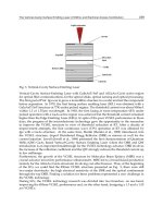
process optimizer is sending a target to one of the outputs. Figures 2 and 3 show the output
and input responses respectively for the two controllers when the system starts from a

steady state where the outputs are outside their zones. It is clear that the conventional MPC
cannot stabilize the plant corresponding to model
1
Θ
when the controller uses model
3
Θ
to
calculate the output predictions. However, the proposed robust controller performs quite
well and is able to bring the three outputs to their zones

0 5 10 15 20 25 30 35 40 45 50
500
550
y1
time (min)
0 5 10 15 20 25 30 35 40 45 50
400
600
800
y2
time (min)
0 5 10 15 20 25 30 35 40 45 50
0
500
1000
y3
time (min)

Fig. 2. Controlled outputs for the nominal (- - -) and robust (⎯⎯) MPC.

We now concentrate our analysis on the application of the proposed controller to the FCC
system. As was defined in Eq. (5), each of the three models produces an input feasible set,
whose intersection constitutes the restricted input feasible set of the controller. These sets
have different shapes and sizes for different stationary operating points (since the
disturbance
()
n
dk is included into Eq. (5), except for the true model case, where the input
feasible set remains unmodified as the estimated states exactly match the true states. The
closed loop simulation begins at u
ss
=[230.5977 60.2359] and y
ss
=[549.5011 704.2756
690.6233], which are values taken from the real FCC system. For such an operating point, the
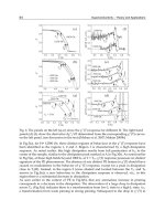
input feasible set corresponding to models 1, 2 and 3 are depicted in Figure 4. These sets are
quite distinct from each other, which results in an empty restricted feasible input set for the
controller (
(
)
(
)
(
)
123uu u u
ϑ
ϑΘ ϑΘ ϑΘ
= ∩∩). This means that, we cannot find an input that,
Robust Control, Theory and Applications

364
taking into account the gains of all the models and all the estimated states, satisfies the
output constraints.

0 5 10 15 20 25 30 35 40 45 50
150
200
250
u1
time (min)
0 5 10 15 20 25 30 35 40 45 50
20
40
60
80
100
u2
time (min)

Fig. 3. Manipulated inputs for the nominal (- - -) and robust (⎯⎯) MPC.


Fig. 4. Input feasible sets of the FCC system
(
)
1u
ϑ
θ
(
)

2u
ϑ
θ
(
)
3u
ϑ
θ
Robust Model Predictive Control for Time Delayed Systems
with Optimizing Targets and Zone Control

365
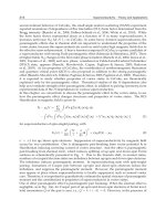
The first objective of the control simulation is to stabilize the system input at
[
]
165 60
a
des
u = . This input corresponds to the output [520 606.8 577.6]y
=
for the true
system
(
)
1
Θ
, which results in the input feasible sets shown in Figure 5a. In this figure, it can
be seen that the input feasible set corresponding to model 1 is the same as in Fig. 4, while the
sets corresponding to the other models adapt their shape and size to the new steady state.
Once the system is stabilized at this new steady state, we simulate a step change in the

target of the input (at time step k=50 min). The new target is given by
[175 64]
b
des
u =
, and
the corresponding input feasible sets are shown in Figure 5b. In this case, it can be seen that
the new target remains inside the new input feasible set
b
u
ϑ
, which means that the cost can
be guided to zero for the true model. Finally, at time step k=100 min, when the system
reaches the steady state, a different input target is introduced ( [175 58]
c
des
u = ). Differently
from the previous targets, this new target is outside the input feasible set
c
u
ϑ
, as can be seen
in Figure 5c. Since in this case, the cost cannot be guided to zero and the output
requirements are more important than the input ones, the inputs are stabilized in a feasible
point as close as possible to the desired target. This is an interesting property of the
controller as such a change in the target is likely to occur in the real plant operation.

Fig. 5. (a): Initial input feasible sets; (b): Input feasible sets when the first input target is
changed; and (c): Input feasible sets when the second input target is changed.
(
)
1
a
u
ϑ
θ
(
)
2
a
u
ϑ
θ
(
)
3
a
u
ϑ
θ
a
des
u
()
1
b
u

ϑ
θ

(
)
2
b
u
ϑ
θ
()
3
b
u
ϑ
θ

b
des
u
c
des
u
final stationary
in
p
ut u
(
)
1

c
u
ϑ
θ
(
)
2
c
u
ϑ
θ
(
)
3
c
u
ϑ
θ
Robust Control, Theory and Applications

366
0 50 100 150
500
550
y1
time (min)
0 50 100 150
600
650
700

y2
time (min)
0 50 100 150
500
600
700
y3
time
(
min
)

Fig. 6. Controlled outputs and set points for the FCC subsystem with modified input target.

0 50 100 150
160
180
200
220
240
u1
time (min)
0 50 100 150
50
60
70
80
u2
time (min)

Fig. 7. Manipulated inputs for the FCC subsystem with different input target.
Figure 6 shows the true system outputs (solid line), the set point variables (dotted line) and
the output zones (dashed line) for the complete sequence of changes. Figure 7, on the other
hand, shows the inputs (solid line), and the input targets (dotted line) for the same
sequence. As was established in Theorem 1, the cost function corresponding to the true
system is strictly decreasing, and this can be seen in Figure 8. In this figure, the solid line
Robust Model Predictive Control for Time Delayed Systems
with Optimizing Targets and Zone Control

367
represents the true cost function, while the dotted line represents the cost corresponding to
model 3. It is interesting to observe that this last cost function is not decreasing, since the
estimated state does not match exactly the true state. Note also that in the last period of
time, the cost does not reach zero, as the new target is not inside the input feasible set.

0 50
0
0.5
1
1.5
2
2.5
x 10
7
Vk
time (min)
60 80 100
0
0.5
1

1.5
2
2.5
3
3.5
4
4.5
5
x 10
4
Vk
100 150
0
1
2
3
4
5
6
7
8
x 10
5
Vk
time (min)

Fig. 8. Cost function corresponding to the true system (solid line) and cost corresponding to
model 3 (dotted line).

Output y

min
y
max
y
1
(ºC) 510 550
y
2
(ºC) 400 500
y
3
(ºC) 350 500
Table 3. New output zones for the FCC subsystem
Next, we simulate a change in the output zones. The new bounds are given in Table 3.
Corresponding to the new control zones, the input feasible set changes its dimension and
shape significantly. In Figure 9,
(
)
1
a
u
ϑ
Θ
corresponds to the initial feasible set for the true
model, and
(
)
1
d
u

ϑ
Θ
,
(
)
2
d
u
ϑ
Θ
and
(
)
3
d
u
ϑ
Θ
represent the new input feasible sets for the three
models considered in the robust controller. Since the input target is outside the input
feasible set
(
)
(
)
(
)
123
dd d d
uu u u

ϑ
ϑΘ ϑΘ ϑΘ
= ∩∩, it is not possible to guide the system to a point
in which the control cost is null at the end of the simulation time. When the output weight
S
y
is as large as the input weight S
u
, all the outputs are guided to their corresponding zones,
while the inputs show a steady state offset with respect to the target
a
des
u . The complete
behavior of the outputs and inputs of the FCC subsystem, as well as the output set-points,
can be seen in Figures 10 and 11, respectively when
(
)
3
10* 111
y
Sdiag= and
()
3
10 * 1 1
u
Sdiag= . The final stationary value of the input is u= [155 84], which represents
the closest feasible input value to the target
a
des
u . Finally, Figure 12 shows the control cost of

Robust Control, Theory and Applications

368
the two simulated time periods. Observe that in the last period of time (from 51min to 100
min) the true cost function does not reach zero since the change in the operating point
prevents the input and output constraints to be satisfied simultaneously.


Fig. 9. Input feasible sets for the FCC subsystem when a change in the output zones is
introduced.

0 10 20 30 40 50 60 70 80 90 100
500
550
y1
time (min)
0 10 20 30 40 50 60 70 80 90 100
400
600
y2
time (min)
0 10 20 30 40 50 60 70 80 90 100
400
600
y3
time
(
min
)

Fig. 10. Controlled outputs and set points for the FCC subsystem with modified zones.
a
des
u
final
stationary u

(
)
1
d
u
ϑ
θ
(
)
2
d
u
ϑ
θ
(
)
3
d
u
ϑ
θ
(
)

1
a
u
ϑ
θ
Robust Model Predictive Control for Time Delayed Systems
with Optimizing Targets and Zone Control

369
0 10 20 30 40 50 60 70 80 90 100
100
150
200
250
u1
time (min)
0 10 20 30 40 50 60 70 80 90 100
40
60
80
100
u2
time (min)

Fig. 11. Manipulated inputs for the FCC subsystem with modified output zones.

10 20 30 40 50
0
1
2

3
4
5
6
7
8
9
10
x 10
7
Vk
time
(
min
)
60 70 80 90 100
0
0.5
1
1.5
2
2.5
3
x 10
8
Vk
time
(
min
)

Fig. 12. Cost function for the FCC subsystem with modified zones. True cost function (solid
line); Cost function of Model 3 (dotted line).
7. Conclusion
In this chapter, a robust MPC previously presented in the literature was extended to the
output zone control of time delayed system with input targets. To this end an extended
Robust Control, Theory and Applications

370
model that incorporates additional states to account for the time delay is presented. The
control structure assumes that model uncertainty can be represented as a discrete set of
models (multi-model uncertainty). The proposed approach assures both, recursive
feasibility and stability of the closed loop system. The main idea consists in using an
extended set of variables in the control optimization problem, which includes the set point
to each predicted output. This approach introduces additional degrees of freedom in the
zone control problem. Stability is achieved by imposing non-increasing cost constraints that
prevent the cost corresponding to the true plant to increase. The strategy was shown, by
simulation, to have an adequate performance for a 2x3 subsystem of a typical industrial
system.
8. References
Badgwell T. A. (1997). Robust model predictive control of stable linear systems. International
Journal of Control, 68, 797-818.
González A. H.; Odloak D.; Marchetti J. L. & Sotomayor O. (2006). IHMPC of a Heat-
Exchanger Network. Chemical Engineering Research and Design, 84 (A11), 1041-1050.
González A. H. & Odloak D. (2009). Stable MPC with zone control. Journal of Process
Control, 19, 110-122.
González A. H.; Odloak D. & Marchetti J. L. (2009) Robust Model Predictive Control with
zone control. IET Control Theory Appl., 3, (1), 121–135.
González A. H.; Odloak D. & Marchetti J. L. (2007). Extended robust predictive control of
integrating systems. AIChE Journal, 53 1758-1769.

Kassmann D. E.; Badgwell T. & Hawkings R. B. (2000). Robust target calculation for model
predictive control. AIChE Journal, 45 (5), 1007-1023.
Muske K.R. & Badgwell T. A. (2002). Disturbance modeling for offset free linear model
predictive control. Journal of Process Control, 12, 617-632.
Odloak D. (2004). Extended robust model predictive control. AIChE Journal, 50 (8) 1824-1836.
Pannochia G. & Rawlings J. B. (2003). Disturbance models for offset-free model-predictive
control. AIChE Journal, 49, 426-437.
Qin S.J. & Badgwell T. A. (2003). A Survey of Industrial Model Predictive Control
Technology, Control Engineering Practice, 11 (7), 733-764.
Rawlings J. B. (2000). Tutorial overview of model predictive control. IEEE Control Systems
Magazine, 38-52.
Sotomayor O. A. Z. & Odloak D. (2005). Observer-based fault diagnosis in chemical plants.
Chemical Engineering Journal, 112, 93-108.
Zanin A. C.; Gouvêa M. T. & Odloak D. (2002). Integrating real time optimization into the
model predictive controller of the FCC system. Contr. Eng. Pract., 10, 819-831.
16
Robust Fuzzy Control of
Parametric Uncertain Nonlinear Systems
Using Robust Reliability Method
Shuxiang Guo
Faculty of Mechanics, College of Science, Air Force Engineering University Xi’an 710051,
P R China
1. Introduction
Stability is of primary importance for any control systems. Stability of both linear and
nonlinear uncertain systems has received a considerable attention in the past decades (see
for example, Tanaka & Sugeno, 1992; Tanaka, Ikeda, & Wang, 1996; Feng, Cao, Kees, et al.
1997; Teixeira & Zak, 1999; Lee, Park, & Chen, 2001; Park, Kim, & Park, 2001; Chen, Liu, &
Tong, 2006; Lam & Leung, 2007, and references therein). Fuzzy logical control (FLC) has
proved to be a successful control approach for a great many complex nonlinear systems.
Especially, the well-known Takagi-Sugeno (T-S) fuzzy model has become a convenient tool

for dealing with complex nonlinear systems. T-S fuzzy model provides an effective
representation of nonlinear systems with the aid of fuzzy sets, fuzzy rules and a set of local
linear models. Once the fuzzy model is obtained, control design can be carried out via the so
called parallel distributed compensation (PDC) approach, which employs multiple linear
controllers corresponding to the locally linear plant models (Hong & Langari, 2000). It has
been shown that the problems of controller synthesis of nonlinear systems described by the
T-S fuzzy model can be reduced to convex problems involving linear matrix inequalities
(LMIs) (Park, Kim, & Park, 2001). Many significant results on the stability and robust control
of uncertain nonlinear systems using T-S fuzzy model have been reported (see for example,
Hong, & Langari, 2000; Park, Kim, & Park, 2001; Xiu & Ren, 2005; Wu & Cai, 2006;
Yoneyama, 2006; 2007), and considerable advances have been made. However, as stated in
Guo (2010), many approaches for stability and robust control of uncertain systems are often
characterized by conservatism when dealing with uncertainties. In practice, uncertainty
exists in almost all engineering systems and is frequently a source of instability and
deterioration of performance. So, uncertainty is one of the most important factors that have
to be taken into account rationally in system analysis and synthesis. Moreover, it has been
shown (Guo, 2010) that the increasing in conservatism in dealing with uncertainties by some
traditional methods does not mean the increasing in reliability. So, it is significant to deal
with uncertainties by means of reliability approach and to achieve a balance between
reliability and performance/control-cost in design of uncertain systems.
In fact, traditional probabilistic reliability methods have ever been utilized as measures of
stability, robustness, and active control effectiveness of uncertain structural systems by
Spencer et al. (1992,1994); Breitung et al. (1998) and Venini & Mariani (1999) to develop