Robust Control Theory and Applications Part 12 pptx

(a) (b)
(c)
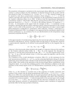
Fig. 1. Procedure of redirectioning of links in a regular network (a) with increasing probability p.Asp
increases the network moves from regular (a) to random (c), becoming small world (b) for a critical value
of p. n=20, k=4
Notice that if BC = c · I
n
, (10) and (11) become:
c
≤−
min
i
|a
ii
|
μ
n
If c
ii
≥ 0 (14)
c
> −
min
i
|a
ii
|
μ
1
If c

ii
< 0 (15)
and hence the stability of MAS is explicitly given as function of the network slowest node
dynamic.
Now we would like to point out the case of undirected topology with symmetric adjacency
matrix U. If we assume A and BC being symmetric, then A
g
is symmetric with real eigenvalue.
Moreover from the field value property (Horn R.A. & Johnson C.R., 1995), let σ
(A)={α
j
}and
σ
(BC)={ν
j
} the eigenvalues set of A and BC, then the eigenvalues of A + μ
i
BC are in the
interval [min
j
{α
j
} + μ
i
min
j
{ν
j
},max
j

{α
j
} + μ
i
max
j
{ν
j
}], for every 1 ≤ i ≤ n ,1≤ j ≤ m.
In this way, there is a bound need to be satisfied by the topology structure, node dynamic and
coupling matrix for MAS stabilization.
428
Robust Control, Theory and Applications
In the literature, the MAS consensuability results have been given in terms of Laplacian
matrix properties. Here, differently, we have given bounds as function of the adjacency
matrix features. Anyway we can use the results on the Laplacian eigenvalue for recasting
the bounds given on the adjacency matrix. To this aim, defined the degree d
i
of i-th node of
an undirected graph as
∑
j
u
ij
, the Laplacian matrix is defined as L = D − U with D is the
diagonal matrix with the degree of node i-th in position i-th. Clearly L is a zero row sums
matrix with non-positive off-diagonal elements. It has at least one zero eigenvalue and all
nonzero eigenvalues have nonnegative real parts. So U
= D − L and being the minimum and
maximum Laplacian eigenvalues respectively bounded by 0 and the highest node degree, we

have:
Lemma 2 Let U the adjacency matrix of undirected and connected graph G
=(V, E, U),with
eigenvalues μ
1
≤ μ
2
≤ ≤ μ
n
,thenresults:
μ
1
(U) ≥ min
i
d
i
−min(max
k,j
{d
k
+ d
j
: (k, j) ∈ E(G)}, n) (16)
μ
n
(U) ≤ max
i
d
i
(17)

Proof Easily follows from the Laplacian eigenvalues bound and the field value property
(Horn R.A. & Johnson C.R., 1995).
4. Simulation validation
In the follows we will present a variety of simulations to validate the above theoretical results
under different kinds of node dynamic and network topology variations. Specifically the MAS
topology variations have been carried out by using the well known Watts-Strogats procedure
described in (Watts & S. H. Strogatz, 1998). In particular, starting from the regular network
topology (p
= 0), by increasing the probability p of rewiring the links, it is possible smoothly
to change its topology into a random one (p
= 1), with small world typically occurring at
some intermediate value. In so doing neither the number of nodes nor the overall number of
edges is changed. In Fig. 1 it shown the results in the case of MAS of 20 nodes with each one
having k
= 4neighbors.
Among the simulation results we focus our attention on the maximum and minimum
eigenvalues of the matrixes U (i.e. μ
n
and μ
1
)andA
g
(i.e. λ
M
and λ
m
) and their bounds
computed by using the results of the previous section. In particular, by Lemma 2, we convey
the bounds on U eigenvalues in bounds on A
g

eigenvalues suitable for the case of time varying
topology structure. We assume in the simulations the matrices A and BC to be symmetric. In
this way, if U eigenvalues are in
[v
1
, v
2
],letσ(A)={α
i
}, σ(BC)={ν
i
}, the eigenvalues of Ag
will be in the interval [min
i
α
i
+ min
j
{v
1
ν
j
, v
2
ν
j
},max
i
α
i

+ max
j
{v
1
ν
j
, v
2
ν
j
}]fori, j = 1, 2,. . . , n.
Notice that, known the interval of variation
[v
1
, v
2
] of the eigenvalues set of U under switching
topologies, we can recast the conditions (8), (9), (12), (13), (6), (7) and to use it for design
purpose. Specifically, given the interval
[v
1
, v
2
] associated to the topology possible variations,
we derive conditions on A or BC for MAS consensuability.
We consider a graph of n
= 400 and k = 4. In the evolving network simulations, we started
with k
= 4andboundedittotheorderofO(log(n)) for setting a sparse graph. In Tab 1 are
drawn the node dynamic and coupling matrices considered in the first set of simulations.

429
Consensuability Conditions of Multi Agent
Systems with Varying Interconnection Topology and Different Kinds of Node Dynamics
10
−3
10
−2
10
−1
10
0
−2
0
2
4
6
8
p
λ
M
(a)
10
−3
10
−2
10
−1
10
0
3

4
5
6
7
8
9
10
11
p
μ
n
(b)
10
−3
10
−2
10
−1
10
0
−20
−15
−10
−5
p
λ
m
(c)
10
−3

10
−2
10
−1
10
0
−16
−14
−12
−10
−8
−6
−4
−2
p
μ
1
(d)
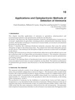
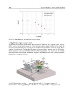
Fig. 2. Case 1. Dashed line: bound on the eigenvalue; continuous line: eigenvalues, (a) Maximum
eigenvalue of A
g
, (b) Maximum eigenvalue of U, (c) Minimum eigenvalue of A
g
,(d)Minimum
eigenvalue of U
0 20 40 60 80 100
0
5
10
15

20
x(t)
t
Fig. 3. Case 1: State dynamic evolution in the time
430
Robust Control, Theory and Applications
10
−3
10
−2
10
−1
10
0
−9
−8
−7
−6
−5
−4
−3
−2
p
λ
M
(a)
10
−3
10
−2

10
−1
10
0
3
4
5
6
7
8
9
10
p
μ
n
(b)
10
−3
10
−2
10
−1
10
0
−28
−26
−24
−22
−20
−18

−16
−14
p
λ
m
(c)
10
−3
10
−2
10
−1
10
0
−16
−14
−12
−10
−8
−6
−4
−2
p
μ
1
(d)
Fig. 4. Case 2. Dashed line: bound on the eigenvalue; continuous line: eigenvalue: (a) Maximum
eigenvalue of A
g
, (b) Maximum eigenvalue of U, (c) Minimum eigenvalue of A

g
,(d)Minimum
eigenvalue of U
A B C
Case 1: -4.1 1 1
Case 2: -12 1 1
Case 3: -6 1 1
Case 4: -6 2 1
Table 1. Node system matrices (A,B,C)
431
Consensuability Conditions of Multi Agent
Systems with Varying Interconnection Topology and Different Kinds of Node Dynamics
10
−3
10
−2
10
−1
10
0
−3
−2
−1
0
1
2
3
4
p
λ

M
(a)
10
−3
10
−2
10
−1
10
0
3
4
5
6
7
8
9
10
p
μ
M
(b)
10
−3
10
−2
10
−1
10
0

−20
−15
−10
p
λ
m
(c)
10
−3
10
−2
10
−1
10
0
−15
−10
−5
p
μ
1
(d)
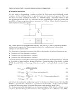
Fig. 5. Case 3. Dashed line: bound on the eigenvalue; continuous line: eigenvalue: (a) Maximum
eigenvalue of A
g
, (b) Maximum eigenvalue of U, (c) Minimum eigenvalue of A
g
,(d)Minimum
eigenvalue of U
0 2 4 6 8 10

0
2
4
6
8
10
t
x(t)
Fig. 6. Case 3: state dynamic evolution in the time
432
Robust Control, Theory and Applications
10
−3
10
−2
10
−1
10
0
2
4
6
8
10
12
14
p
λ
M
(a)

10
−3
10
−2
10
−1
10
0
3
4
5
6
7
8
9
10
p
μ
n
(b)
10
−3
10
−2
10
−1
10
0
−40
−35

−30
−25
−20
−15
−10
p
λ
m
(c)
10
−3
10
−2
10
−1
10
0
−16
−14
−12
−10
−8
−6
−4
−2
p
μ
1
(d)
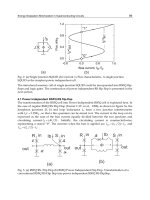
Fig. 7. Case 4. Dashed line: bound on the eigenvalues; continuous line: eigenvalues: (a) Maximum

eigenvalue of A
g
, (b) Maximum eigenvalue of U, (c) Minimum eigenvalue of A
g
,(d)Minimum
eigenvalue of U
In the case 1 (Fig 2), we note as although we start from a stable MAS network, the topology
variation leads the network instability condition (namely λ
M
becomes positive). In Fig. 3 it is
shown the time state evolution of the firsts 10 nodes, under the switching frequency of 1 Hz.
We note as the MAS converges to the consensus state till it is stable, then goes in instability
condition.
In the case 2, we consider a node dynamic faster than the maximum network degree d
M
of
all evolving network topologies from compete to random graph. Notice that although this
assures MAS consensuability as drawn in Fig. 4, it can be much conservative.
In the case 3 (Fig 5), we consider a slower node dynamic than the cases 2. The MAS is robust
stable under topology variations. In Fig. 6 the state dynamic evolution is convergent and the
settling time is about 4.6/
|λ
M
(A
g
)|.
Then we have varied the value for BC by doubling the B matrix value leaving unchanged the
node dynamic matrix. As appears in Fig. 7, the MAS goes in instability condition pointing out
433
Consensuability Conditions of Multi Agent

Systems with Varying Interconnection Topology and Different Kinds of Node Dynamics
10
−3
10
−2
10
−1
10
0
−2
0
2
4
6
p
λ
M
(a)
10
−3
10
−2
10
−1
10
0
2
4
6
8

10
p
μ
n
(b)
10
−3
10
−2
10
−1
10
0
−30
−25
−20
−15
−10
p
λ
m
(c)
10
−3
10
−2
10
−1
10
0

−15
−10
−5
0
p
μ
1
(d)
Fig. 8. Case 5. Dashed line: bound on the eigenvalue; continuous line: eigenvalue: (a) Maximum
eigenvalue of A
g
, (b) Maximum eigenvalue of U, (c) Minimum eigenvalue of A
g
,(d)Minimum
eigenvalue of U
that also the coupling strength can affect the stability (as stated by the conditions (8), (9)) and
that this effect can be amplified by the network topological variations.
A B C
Case 5:

−63
3
−12


1
0


10


Case 6:

−33
3
−6


1
0


10

Case 7:

−33
3
−6


0.25
0


10

Table 2. Node system matrices (A,B,C).
434
Robust Control, Theory and Applications

10
−3
10
−2
10
−1
10
0
1
2
3
4
5
6
7
8
p
λ
M
(a)
10
−3
10
−2
10
−1
10
0
2
3

4
5
6
7
8
9
p
μ
n
(b)
10
−3
10
−2
10
−1
10
0
−22
−20
−18
−16
−14
−12
−10
−8
p
λ
m
(c)

10
−3
10
−2
10
−1
10
0
−14
−12
−10
−8
−6
−4
−2
0
p
μ
1
(d)
Fig. 9. Case 6. Dashed line: bound on the eigenvalue; continuous line: eigenvalue: (a) Maximum
eigenvalue of A
g
, (b) Maximum eigenvalue of U, (c) Minimum eigenvalue of A
g
,(d)Minimum
eigenvalue of U
On the other side, a reduction on BC increases the MAS stability margin. So we can tune
the BC value in order to guarantee stability or desired robust stability MAS margin under a
specified node dynamic and topology network variations. Indeed if BC has eigenvalues above

1,itseffectistoamplifytheeigenvaluesofU and we need a faster node dynamic for assessing
MAS stability. If BC has eigenvalues less of 1, its effect is of attenuation and the node dynamic
can be slower without affecting the network stability.
Now we consider SISO system of second order at the node as shown in Tab.2. In this case the
matrix BC has one zero eigenvalue being the rows linearly dependent.
In the case 5 the eigenvalues of A are α
1
= −4.76 and α
2
= −13.23, the eigenvalues of the
coupling matrix BC are ν
1
= 1andν
2
= 0. In this case the node dynamic is sufficiently fast for
guaranteeing MAS consensuability (Fig. 8). In the case 6, we reduce the node dynamic matrix
A to α
1
= −1.15 e α
2
= −7.85. Fig. 9 shows instability condition for the MAS network. We
435
Consensuability Conditions of Multi Agent
Systems with Varying Interconnection Topology and Different Kinds of Node Dynamics
10
−3
10
−2
10
−1

10
0
−1
−0.5
0
0.5
1
p
λ
M
(a)
10
−3
10
−2
10
−1
10
0
2
3
4
5
6
7
8
9
p
μ
n

(b)
10
−3
10
−2
10
−1
10
0
−11.5
−11
−10.5
−10
−9.5
−9
−8.5
−8
−7.5
−7
−6.5
−6
p
λ
m
(c)
10
−3
10
−2
10

−1
10
0
−14
−12
−10
−8
−6
−4
−2
0
p
μ
1
(d)
Fig. 10. Case 7. Dashed line: bound on the eigenvalue; continuous line: eigenvalue. (a) Maximum
eigenvalue of A
g
, (b) Maximum eigenvalue U, (c) Minimum eigenvalue of A
g
, (d) Minimum eigenvalue
of U
can lead the MAS in stability condition by designing the coupling matrix BC as appear by the
case 7 and the associate Fig. 10.
4.1 Robustness to node fault
Now we deal with the case of node fault. We can state the following Theorem.
Theorem 2 Let A and BC symmetric matrix and G
(V, E, U) an undirected graph. If the MAS
system described by A
g

is stable, it is stable also in the presence of node faults. Moreover the
MAS dynamic becomes faster after the node fault.
Proof Being the graph undirected and A and BC symmetric then A
g
is symmetric. Let
˜
A
g
the
MAS dynamic matrix associated to the network after a node fault.
˜
A
g
is obtained from A
g
by
eliminating the rows and columns corresponding to the nodes went down. So
˜
A
g
is a minor of
A
g
and for the interlacing theorem (Horn R.A. & Johnson C.R., 1995) it has eigenvalues inside
436
Robust Control, Theory and Applications
10
−3
10
−2

10
−1
10
0
−2.2
−2
−1.8
−1.6
−1.4
−1.2
p
λ
M
(a)
10
−3
10
−2
10
−1
10
0
3.8
4
4.2
4.4
4.6
4.8
5
p

μ
n
(b)
10
−3
10
−2
10
−1
10
0
−10
−9.5
−9
−8.5
−8
p
λ
m
(c)
10
−3
10
−2
10
−1
10
0
−4
−3.5

−3
−2.5
−2
p
μ
1
(d)
Fig. 11. Eigenvalues in the case l = 1. Dashed line: eigenvalue in the case of complete topology with
n
= 100; continuous line: eigenvalue in the case of node fault: (a) Maximum eigenvalue of A
g
,(b)
Maximum eigenvalue of U, (c) Minimum eigenvalue of A
g
, (d) Minimum eigenvalue of U
the real interval with extremes the minimum and maximum A
g
eigenvalues. Hence if A
g
is
stable,
˜
A
g
is stable too. Moreover, the maximum eigenvalue of
˜
A
g
is less than one of A
g

.So
the slowest dynamic of the system
˙
x
(t)=
˜
A
g
x(t) is faster than the system
˙
x(t)=A
g
x(t).
In the follows we will show the eigenvalues of MAS dynamic in the presence of node fault.
We consider MAS network with n
= 100. We compare for each evolving network topology
at each time simulation step, the maximum and minimum eigenvalues of A
g
than those ones
resulting with the fault of randomly chosen l nodes. Figures 11 and 12 show the eigenvalues
of system dynamic for the cases l
= 1andl = 50.
Notice that as the eigenvalues of U and A
g
of fault network are inside the real interval
containing the eigenvalues of U and A
g
of the complete graph. In Fig. 13 are shown the time
evolutions of state of the complete and faulted graphs. Notice that the fault network is faster
than the initial network as stated by the analysis of the spectra of A

g
and
˜
A
g
.
437
Consensuability Conditions of Multi Agent
Systems with Varying Interconnection Topology and Different Kinds of Node Dynamics
10
−3
10
−2
10
−1
10
0
−3.5
−3
−2.5
−2
−1.5
−1
p
λ
M
(a)
10
−3
10

−2
10
−1
10
0
2.5
3
3.5
4
4.5
5
p
μ
n
(b)
10
−3
10
−2
10
−1
10
0
−10
−9.5
−9
−8.5
−8
−7.5
p

λ
m
(c)
10
−3
10
−2
10
−1
10
0
−4
−3.5
−3
−2.5
−2
−1.5
p
μ
1
(d)
Fig. 12. Eigenvalues in the case of l = 50. Dashed line: eigenvalue in the case of complete topology with
n
= 100; continuous line: eigenvalue in the case of node fault: (a) Maximum eigenvalue of A
g
,(b)
Maximum eigenvalue of U, (c) Minimum eigenvalue of A
g
, (d) Minimum eigenvalue of U
5. Conclusions

In this book chapter we have investigated the consensuability of the MASs under both the
dynamic agent structure and communication topology variations. Specifically, it has given
consensusability conditions of linear MASs as function of the agent dynamic structure,
communication topology and coupling strength parameters. The theoretical results are given
by transferring the consensusability problem to the stability analysis of LTI-MASs. Moreover,
it is shown that the interplay among consensusability, node dynamic and topology must
be taken into account for MASs stabilization: consensuability of MASs is assessed for
all topologies, dynamic and coupling strength satisfying a pre-specified bound. From the
practical point of view the consensuability conditions can be used for both the analysis
and planning of MASs protocols to guarantee robust stability for a wide range of possible
interconnection topologies, coupling strength and node dynamics. Also, the consensuability
438
Robust Control, Theory and Applications
0 1 2 3 4 5
0
50
100
t
x(t)
0 1 2 3 4 5
−50
0
50
100
t
x(t)
Fig. 13. Time evolution of the state variables for l=50: top Figure: complete graph. Bottom Figure: graph
with fault.
of MAS in the presence of node faults has been analyzed. Simulation scenarios are given to
validate the theoretical results.

Acknowledgement
The author would like to thank Ms. F. Schioppa for valuable discussion.
6.References
J.K. Hedrick, D.H. McMahon, V.K. Narendran, and D. Swaroop. (1990). Longitudinal vehical
controller design for IVHS systems. Proceedings of the American Control Conference,
pages 3107-3112.
P. Kundur. (1994) Power System Stability and Control. McGraw-Hill.
D. Limebeer and Y.S. Hung. (1983). Robust stability of interconnected systems. IEEE Trans.
Automatic Control, pages 710-716.
A. Michel and R. Miller. (1977). Qualitative analysis of large scale dynamical systems. Academic
Press.
P.J. Moylan and D.J. Hill. (1978). Stability criteria for large scale systems. IEEE Trans. Automatic
Control, pages 143-149.
F. Paganini, J. Doyle, and S. Low. (2001). Scalable laws for stable network congestion control.
Proceedings of the IEEE Conference on Decision and Control, pages 185-190, 2001.
439
Consensuability Conditions of Multi Agent
Systems with Varying Interconnection Topology and Different Kinds of Node Dynamics
M. Vidyasagar. (1977). L2 stability of interconnected systems using a reformulation of the passivity
theorem. IEEE Transactions on Circuits and Systems, 24, 637-645.
D. ˚uSiljak. (1978). Large-Scale Dynamic Systems. Elsevier North-Holland.
J.C. Willems. (1976). Stability of large-scale interconnected systems
Saber R.O., Murray R.M. (2004). Consensus Problems in Networks of Agents with Switching
Topology and Time-Delays, IEEE Transactions on Automatic Control, Vol 49, 9.
Z. Lin, M. Brouke, and B. Francis, (2004). Local control strategies for groups of mobile autonomous
agents., Transactions on Automatic Control, 49, vol 4, pages: 622
˝
U-629.
V. Blondel, J. M. Hendrickx, A. Olshevsky, and J. N. Tsitsiklis, (2005) Convergence in multiagent
coordination, consensus, and flocking, 44th IEEE Conference on Decision and Control

and European Control Conference, pages 2996
˝
U-3000.
A. V. Savkin, (2004) Coordinated collective motion of groups of autonomous mobile robots: analysis of
VicsekŠs model., Transactions on Automatic Control, Vol 49, 6, pages: 981-
˝
U982.
J. N. Tsitsiklis, D. P. Bertsekas, M. Athans, (1986). Distributed Asynchronous Deterministic
and Stochastic Gradient Optimization Algorithms, Transactions on Automatic Control,
pages. 803-
˝
U812.
C. C. Cheaha, S. P. Houa, and J. J. E. Slotine, (2009). Region-based shape control for a swarm of
robots., Automatica, Vol. 45, 10, pages: 2406-
˝
U2411.
Ren, W., (2009). Collective Motion From Consensus With Cartesian Coordinate Coupling ., IEEE
Transactions on Automatic Control. Vol. 54, 6, pages: 1330–1335.
S. E. Tuna, (2008). LQR-based coupling gain for synchronization of linear systems, Available at:
/>Luca Scardovi, Rodolphe Sepulchre, (2009) Synchronization in networks of identical linear systems
Automatica, Volume 45, Issue 11, Pages 2557-2562
W. Ren and R. W. Beard, (2005), Consensus seeking in multiagent systems under dynamically
changing interaction topologies, IEEE Trans. Automatic Control, vol. 50, no. 5, pp.
655-661.
Ya Zhanga and Yu-Ping Tian, (2009). Consentability and protocol design of multi-agent systems
with stochastic switching topology., Automatica, Vol. 45, 5, 2009, Pages 1195–1201.
R. Cogill, S. Lall, (2004). Topology independent controller design for networked systems, IEEE
Conference on Decision and Control, Atlantis, Paradise Island, Bahamas, Dicembre
2004
D. J. Watts, S. H. Strogatz, (1998). Collective dynamics of small world networks, Nature - Macmillan

Publishers Ltd, Vol. 393, Giugno 1998.
Horn R.A. and Johnson C.R., (1995). Topics in Matrix Analysis Cambridge University Press
1995.
440
Robust Control, Theory and Applications
Bogdan Sasu
*
and Adina Lumini¸ta Sasu
Department of Mathematics, Faculty of Mathematics and Computer Science, West
University of Timi¸soara, V. Pârvan Blvd. No. 4 300223 Timi¸soara
Romania
1. Introduction
The aim of this chapter is to present several interesting connections between the input-output
stability properties and the stabilizability and detectability of variational control systems,
proposing a new perspective concerning the interference of the interpolation methods in
control theory and extending the applicability area of the input-output methods in the stability
theory.
Indeed, let X be a Banach space, let
(Θ, d) be a locally compact metric space and let E = X ×Θ.
We denote by
B(X) the Banach algebra of all bounded linear operators on X.IfY, U are two
Banach spaces, we denote by
B(U, Y) the space of all bounded linear operators from U into Y
and by
C
s
(Θ, B(U, Y)) the space of all continuous bounded mappings H : Θ →B(U, Y).With
respect to the norm
||| H||| := sup
θ∈Θ

|| H(θ)||, C
s
(Θ, B(U, Y)) is a Banach space.
If H
∈C
s
(Θ, B(U, Y)) and Q ∈C
s
(Θ, B(Y, Z)) we denote by QH the mapping Θ  θ →
Q(θ)H(θ). It is obvious that QH ∈C
s
(Θ, B(U, Z)) .
Definition 1.1. Let J
∈{R
+
, R}. A continuous mapping σ : Θ × J → Θ is called aflowon Θ
if σ
(θ,0)=θ and σ(θ, s + t)=σ(σ(θ, s), t),forall(θ, s, t) ∈ Θ × J
2
.
Definition 1.2. Apairπ
=(Φ, σ) is called a linear skew-product flow on E = X × Θ if σ is a
flow on Θ and Φ : Θ
×R
+
→B(X) satisfies the following conditions:
(i) Φ
(θ,0)=I
d
, the identity operator on X,forallθ ∈ Θ;

(ii) Φ
(θ, t + s)=Φ(σ(θ, t), s)Φ(θ, t),forall(θ, t, s) ∈ Θ × R
2
+
(the cocycle identity);
(iii)
(θ, t) → Φ(θ, t)x is continuous, for every x ∈ X;
(iv) there are M
≥ 1andω > 0suchthat||Φ(θ,t)|| ≤ Me
ωt
,forall(θ, t) ∈ Θ ×R
+
.
The mapping Φ is called the cocycle associated to the linear skew-product flow π
=(Φ, σ).
Let L
1
loc
(R
+
, X) denote the linear space of all locally Bochner integrable functions u : R
+
→ X.
Let π
=(Φ, σ) be a linear skew-product flow on E = X ×Θ. We consider the variational
integral system
(S
π
) x
θ

(t; x
0
, u)=Φ(θ, t)x
0
+

t
0
Φ(σ(θ, s), t −s)u(s) ds, t ≥ 0, θ ∈ Θ
*
The work is supported by The National Research Council CNCSIS-UEFISCSU, PN II Research Grant
ID 1081 code 550.
On Stabilizability and Detectability of
Variational Control Systems
19
with u ∈ L
1
loc
(R
+
, X) and x
0
∈ X.
Definition 1.3. The system
(S
π
) is said to be uniformly exponentially stable if there are N, ν > 0
such that
||x
θ

(t; x
0
,0)|| ≤ Ne
−νt
||x
0
||, ∀(θ, t) ∈ Θ ×R
+
, ∀x
0
∈ X.
Remark 1.4. It is easily seen that the system
(S
π
) is uniformly exponentially stable if and only
if there are N, ν
> 0suchthat||Φ(θ, t)|| ≤ Ne
−νt
,forall(θ, t) ∈ Θ ×R
+
.
If π
=(Φ, σ) is a linear skew-product flow on E = X ×Θ and P ∈C
s
(Θ, B(X)), then there
exists a unique linear skew-product flow denoted π
P
=(Φ
P
, σ) on X × Θ such that this

satisfies the variation of constants formula:
Φ
P
(θ, t)x = Φ(θ, t)x +

t
0
Φ(σ(θ, s), t −s)P( σ(θ, s))Φ
P
(θ, s)xds (1.1)
and respectively
Φ
P
(θ, t)x = Φ(θ, t)x +

t
0
Φ
P
(σ(θ, s), t −s)P( σ(θ, s))Φ(θ, s)xds (1.2)
for all (x, θ, t) ∈E×R
+
.Moreover,ifM, ω are the exponential growth constants given by
Definition 1.2 (iv) for π,then
||Φ
P
(θ, t)|| ≤ Me
(ω+M || P||)t
, ∀(θ, t) ∈ Θ × R
+

.
The perturbed linear skew-product flow π
P
=(Φ
P
, σ) is obtained inductively (see Theorem
2.1 in (Megan et al., 2002)) via the formula
Φ
P
(θ, t)=
∞
∑
n=0
Φ
n
(θ, t),
where
Φ
0
(θ, t)x = Φ(θ, t)x and Φ
n
(θ, t)x =

t
0
Φ(σ(θ, s), t −s) P(σ(θ, s)) Φ
n−1
(θ, s)xds, n ≥ 1
for every
(x, θ) ∈Eand t ≥ 0.

Let U, Y be two Banach spaces, let B
∈C
s
(Θ, B(U, X)) and C ∈C
s
(Θ, B(X, Y)).Weconsider
the variational control system
(π, B, C) described by the following integral model
⎧
⎨
⎩
x
(θ, t, x
0
, u)=Φ(θ, t)x
0
+

t
0
Φ(σ(θ, s), t −s)B( σ(θ, s))u(s) ds
y
(θ, t, x
0
, u)=C(σ(θ, t)) x(θ, t, x
0
, u)
where t ≥ 0, (x
0
, θ) ∈Eand u ∈ L

1
loc
(R
+
, U).
Two fundamental concepts related to the asymptotic behavior of the associated perturbed
systems (see (Clark et al., 2000), (Curtain & Zwart, 1995), (Sasu & Sasu, 2004)) are described
by stabilizability and detectability as follows:
Definition 1.5. The system
(π, B, C) is said to be:
(i) stabilizable if there exists a mapping F
∈C
s
(Θ, B(X, U)) such that the system (S
π
BF
) is
uniformly exponentially stable;
(ii) detectable if there exists a mapping K
∈C
s
(Θ, B(Y, X)) such that the system (S
π
KC
) is
uniformly exponentially stable.
442
Robust Control, Theory and Applications
Remark 1.6. (i) The system (π, B, C) is stabilizable if and only if there exists a mapping F ∈
C

s
(Θ, B(X, U)) and two constants N, ν > 0 such that the perturbed linear skew-product flow
π
BF
=(Φ
BF
, σ) has the property
||Φ
BF
(θ, t)|| ≤ Ne
−νt
, ∀(θ, t) ∈ Θ ×R
+
;
(ii) The system
(π, B, C) is detectable if and only if there exists a mapping K ∈C
s
(Θ, B(Y, X))
and two constants N, ν > 0 such that the perturbed linear skew-product flow π
KC
=(Φ
KC
, σ)
has the property
||Φ
KC
(θ, t)|| ≤ Ne
−νt
, ∀(θ, t) ∈ Θ × R
+

.
In the present work we will investigate the connections between the stabilizability and
the detectability of the variational control system
(π, B, C) and the asymptotic properties
of the variational integral system
(S
π
). We propose a new method based on input-output
techniques and on the behavior of some associated operators between certain function spaces.
We will present a distinct approach concerning the stabilizability and detectability problems
for variational control systems, compared with those in the existent literature, working with
several representative classes of translations invariant function spaces (see Section 2 in (Sasu,
2008) and also (Bennet & Sharpley, 1988)) and thus we extend the applicability area, providing
new perspectives concerning this framework.
A special application of our main results will be the study of the connections between
the exponential stability and the stabilizability and detectability of nonautonomous control
systems in infinite dimensional spaces. The nonautonomous case treated in this chapter will
include as consequences many interesting situations among which we mention the results
obtained by Clark, Latushkin, Montgomery-Smith and Randolph (see (Clark et al., 2000))
and the authors (see (Sasu & Sasu, 2004)) concerning the connections between stabilizability,
detectability and exponential stability.
2. Preliminaries on Banach function spaces and auxiliary results
In what follows we recall several fundamental properties of Banach function spaces and we
introduce the main tools of our investigation. Indeed, let
M(R
+
, R) be the linear space of all
Lebesgue measurable functions u : R
+
→ R, identifying the functions equal a.e.

Definition 2.1. A linear subspace B of
M(R
+
, R) is called a normed function space,ifthereisa
mapping
|·|
B
: B → R
+
such that:
(i) |u|
B
= 0 if and only if u = 0 a.e.;
(ii) |αu|
B
= |α||u|
B
,forall(α, u) ∈ R × B;
(iii) |u + v|
B
≤|u|
B
+ |v|
B
,forallu, v ∈ B;
(iv) if |u(t)|≤|v(t)| a.e. t ∈ R
+
and v ∈ B,thenu ∈ B and |u|
B
≤|v|

B
.
If
(B, |·|
B
) is complete, then B is called a Banach function space.
Remark 2.2. If
(B, |·|
B
) is a Banach function space and u ∈ B then |u(·)|∈B.
A remarkable class of Banach function spaces is represented by the translations invariant
spaces. These spaces have a special role in the study of the asymptotic properties of the
dynamical systems using control type techniques (see Sasu (2008), Sasu & Sasu (2004)).
443
On Stabilizability and Detectability of Variational Control Systems
Definition 2.3. A Banach function space (B, |·|
B
) is said to be invariant to translations if for
every u : R
+
→ R and every t > 0, u ∈ B if and only if the function
u
t
: R
+
→ R, u
t
(s)=

u

(s − t) , s ≥ t
0,s
∈ [0, t)
belongs to B and |u
t
|
B
= |u|
B
.
Let C
c
(R
+
, R) denote the linear space of all continuous functions v : R
+
→ R with compact
support contained in R
+
and let L
1
loc
(R
+
, R) denote the linear space of all locally integrable
functions u : R
+
→ R.
We denote by
T (R

+
) the class of all Banach function spaces B which are invariant to
translations and satisfy the following properties:
(i) C
c
(R
+
, R) ⊂ B ⊂ L
1
loc
(R
+
, R);
(ii) if B
\ L
1
(R
+
, R) = ∅ then there is a continuous function δ ∈ B \ L
1
(R
+
, R).
For every A
⊂ R
+
we denote by χ
A
the characteristic function of the set A.
Remark 2.4. (i) If B

∈T(R
+
),thenχ
[0,t)
∈ B,forallt > 0.
(ii) Let B
∈T(R
+
), u ∈ B and t > 0. Then, the function
˜
u
t
: R
+
→ R,
˜
u
t
(s)=u(s + t) belongs
to B and
|
˜
u
t
|
B
≤|u|
B
(see (Sasu, 2008), Lemma 5.4).
Definition 2.5. (i) Let u, v

∈M(R
+
, R). We say that u and v are equimeasurable if for every
t
> 0thesets{s ∈ R
+
: |u(s)| > t} and {s ∈ R
+
: |v(s)| > t} have the same measure.
(ii) A Banach function space
(B, |·|
B
) is rearrangement invariant if for every equimeasurable
functions u, v : R
+
→ R
+
with u ∈ B we have that v ∈ B and |u|
B
= |v|
B
.
We denote by
R(R
+
) the class of all Banach function spaces B ∈T(R
+
) which are
rearrangement invariant.
A remarkable class of rearrangement invariant function spaces is represented by the so-called

Orlicz spaces which are introduced in the following remark:
Remark 2.6. Let ϕ : R
+
→ R
+
be a non-decreasing left-continuous function, which is
not identically zero on
(0, ∞).TheYoung function associated with ϕ is defined by Y
ϕ
(t)=

t
0
ϕ(s) ds. For every u ∈M(R
+
, R) let M
ϕ
(u) :=

∞
0
Y
ϕ
(|u(s)|) ds.ThesetO
ϕ
of all
u
∈M(R
+
, R) with the property that there is k > 0suchthatM

ϕ
(ku ) < ∞,isalinear
space. With respect to the norm
|u|
ϕ
:= inf{k > 0:M
ϕ
(u/k) ≤ 1}, O
ϕ
is a Banach space,
called the Orlicz space associated with ϕ.
The Orlicz spaces are rearrangement invariant (see (Bennet & Sharpley, 1988), Theorem 8.9).
Moreover, it is well known that, for every p
∈ [1, ∞],thespaceL
p
(R
+
, R) is a particular case
of Orlicz space.
Let now
(X, ||·||) be a real or complex Banach space. For every B ∈T(R
+
) we denote
by B
(R
+
, X) , the linear space of all Bochner measurable functions u : R
+
→ X with the
property that the mapping N

u
: R
+
→ R
+
, N
u
(t)=||u(t)||lies in B. Endowed with the norm
||u||
B(R
+
,X)
:= |N
u
|
B
, B(R
+
, X) is a Banach space.
Let
(Θ, d) be a metric space and let E = X ×Θ.Letπ =(Φ, σ) be a linear skew-product flow
on
E = X × Θ. We consider the variational integral system
(S
π
) x
θ
(t; x
0
, u)=Φ(θ, t)x

0
+

t
0
Φ(σ(θ, s), t −s)u(s) ds, t ≥ 0, θ ∈ Θ
444
Robust Control, Theory and Applications
with u ∈ L
1
loc
(R
+
, X) and x
0
∈ X.
An important stability concept related with the asymptotic behavior of dynamical systems is
described by the following concept:
Definition 2.7. Let W
∈T( R
+
). The system (S
π
) is said to be completely (W(R
+
, X) ,
W
(R
+
, X))-stable if the following assertions hold:

(i) for every u
∈ W(R
+
, X) and every θ ∈ Θ the solution x
θ
(·;0,u) ∈ W(R
+
, X);
(ii) there is λ
> 0suchthat|| x
θ
(·;0,u)||
W(R
+
,X)
≤ λ||u||
W(R
+
,X)
,forall(u, θ) ∈ W(R
+
, X) ×
Θ.
A characterization of uniform exponential stability of variational systems in terms of the
complete stability of a pair of function spaces has been obtained in (Sasu, 2008) (see Corollary
3.19) and this is given by:
Theorem 2.8. Let W
∈R(R
+
). The system (S

π
) is uniformly exponentially stable if and only if
(S
π
) is completely (W(R
+
, X) , W(R
+
, X))-stable.
The problem can be also treated in the setting of the continuous functions. Indeed, let
C
b
(R
+
, R) be the space of all bounded continuous functions u : R
+
→ R .LetC
0
(R
+
, R)
be the space of all continuous functions u : R
+
→ R with lim
t→∞
u(t)=0andletC
00
(R
+
, R) :=

{
u ∈ C
0
(R
+
, R) : u(0)=0}.
Definition 2.9. Let V
∈{C
b
(R
+
, R), C
0
(R
+
, R), C
00
(R
+
, R)}. The system (S
π
) is said to be
completely
(V(R
+
, X) , V(R
+
, X))-stable if the following assertions hold:
(i) for every u
∈ V(R

+
, X) and every θ ∈ Θ the solution x
θ
(·;0,u) ∈ V(R
+
, X) ;
(ii) there is λ
> 0suchthat||x
θ
(·;0,u)||
V(R
+
,X)
≤ λ||u||
V(R
+
,X)
,forall(u, θ) ∈ V(R
+
, X) ×Θ.
For the proof of the next result we refer to Corollary 3.24 in (Sasu, 2008) or, alternatively, to
Theorem 5.1 in (Megan et al., 2005).
Theorem 2.10. Let V
∈{C
b
(R
+
, R), C
0
(R

+
, R), C
00
(R
+
, R)}. The system (S
π
) is uniformly
exponentially stable if and only if
(S
π
) is completely (V(R
+
, X) , V(R
+
, X))-stable.
Remark 2.11. Let W
∈R(R
+
) ∪{C
0
(R
+
, X) , C
00
(R
+
, X) , C
b
(R

+
, X)}. If the system (S
π
) is
uniformly exponentially stable then for every θ
∈ Θ the linear operator
P
θ
W
: W(R
+
, X) → W(R
+
, X) , (P
θ
W
u)(t)=

t
0
Φ(σ(θ, s), t −s)u(s ) ds
is correctly defined and bounded. Moreover, if λ
> 0 is given by Definition 2.7 or respectively
by Definition 2.9, then we have that sup
θ∈Θ
||P
θ
W
|| ≤ λ.
These results have several interesting applications in control theory among we mention those

concerning the robustness problems (see (Sasu, 2008)) which lead to an inedit estimation of
the lower bound of the stability radius, as well as to the study of the connections between
stability and stabilizability and detectability of associated control systems, as we will see in
what follows. It worth mentioning that these aspects were studied for the very first time for
the case of systems associated to evolution operators in (Clark et al., 2000) and were extended
for linear skew-product flows in (Megan et al., 2002).
445
On Stabilizability and Detectability of Variational Control Systems
3. Stabilizability and detectability of variational control systems
As stated from the very beginning, in this section our attention will focus on the connections
between stabilizability, detectability and the uniform exponential stability. Let X be a Banach
space, let
(Θ, d) be a metric space and let π =(Φ, σ) be a linear skew-product flow on E =
X ×Θ. We consider the variational integral system
(S
π
) x
θ
(t; x
0
, u)=Φ(θ, t)x
0
+

t
0
Φ(σ(θ, s), t −s)u(s) ds, t ≥ 0, θ ∈ Θ
with u
∈ L
1

loc
(R
+
, X) and x
0
∈ X.
Let U, Y be Banach spaces and let B
∈C
s
(Θ, B(U, X)), C ∈C
s
(Θ, B(X, Y)).Weconsiderthe
variational control system
(π, B, C) described by the following integral model
⎧
⎨
⎩
x
(θ, t, x
0
, u)=Φ(θ, t)x
0
+

t
0
Φ(σ(θ, s), t −s)B( σ(θ, s))u(s) ds
y
(θ, t, x
0

, u)=C(σ(θ, t)) x(θ, t, x
0
, u)
where t ≥ 0, (x
0
, θ) ∈Eand u ∈ L
1
loc
(R
+
, U).
According to Definition 1.5 it is obvious that if the system
(S
π
) is uniformly exponentially
stable, then the control system
(π, B, C) is stabilizable (via the trivial feedback F ≡ 0) and
this is also detectable (via the trivial feedback K
≡ 0). The natural question arises whether the
converse implication holds.
Example 3.1. Let X
= R, Θ = R and let σ(θ, t)=θ + t.Let(S
π
) be a variational integral
system such that Φ
(θ, t)=I
d
(the identity operator on X), for all (θ, t) ∈ Θ × R
+
.LetU =

Y = X and let B(θ)=C(θ)=I
d
,forallθ ∈ Θ.Letδ > 0. By considering F(θ)=−δ I
d
,forall
θ
∈ Θ, from relation (1.1), we obtain that
Φ
BF
(θ, t)x = x −δ

t
0
Φ
BF
(θ, s)xds, ∀t ≥ 0
for every
(x, θ) ∈E. This implies that Φ
BF
(θ, t)x = e
−δt
x,forallt ≥ 0andall(x, θ) ∈E,
so the perturbed system
(S
π
BF
) is uniformly exponentially stable. This shows that the system
(π, B, C) is stabilizable.
Similarly, if δ
> 0, for K(θ)=−δ I

d
,forallθ ∈ Θ, we deduce that the variational control
system
(π, B, C) is also detectable.
In conclusion, the variational control system
(π, B, C) is both stabilizable and detectable, but
for all that, the variational integral system
(S
π
) is not uniformly exponentially stable.
It follows that the stabilizability or/and the detectability of the control system
(π, B, C) are
not sufficient conditions for the uniform exponential stability of the system
(S
π
). Naturally,
additional hypotheses are required. In what follows we shall prove that certain input-output
conditions assure a complete resolution to this problem. The answer will be given employing
new methods based on function spaces techniques.
Indeed, for every θ
∈ Θ,wedefine
P
θ
: L
1
loc
(R
+
, X) → L
1

loc
(R
+
, X) , (P
θ
w)(t)=

t
0
Φ(σ(θ, s), t −s)w(s) ds
446
Robust Control, Theory and Applications
and respectively
B
θ
: L
1
loc
(R
+
, U) → L
1
loc
(R
+
, X) , (B
θ
u)(t)=B(σ(θ, t))u(t)
C
θ

: L
1
loc
(R
+
, X) → L
1
loc
(R
+
, Y), (C
θ
v)(t)=C(σ(θ, t))v(t).
We also associate with the control system S
=(π, B, C) three families of input-output
mappings, as follows: the left input-output operators
{L
θ
}
θ∈Θ
defined by
L
θ
: L
1
loc
(R
+
, U) → L
1

loc
(R
+
, X) , L
θ
:= P
θ
B
θ
the right input-output operators {R
θ
}
θ∈Θ
given by
R
θ
: L
1
loc
(R
+
, X) → L
1
loc
(R
+
, Y), R
θ
:= C
θ

P
θ
and respectively the global input-output operators {G
θ
}
θ∈Θ
defined by
G
θ
: L
1
loc
(R
+
, U) → L
1
loc
(R
+
, Y), G
θ
:= C
θ
P
θ
B
θ
.
A fundamental stability concept for families of linear operators is given by the following:
Definition 3.2. Let Z

1
, Z
2
be two Banach spaces and let W ∈T(R
+
) be a Banach function
space. A family of linear operators
{O
θ
: L
1
loc
(R
+
, Z
1
) → L
1
loc
(R
+
, Z
2
)}
θ∈Θ
is said to be
(W(R
+
, Z
1

), W(R
+
, Z
2
))-stable if the following conditions are satisfied:
(i) for every α
1
∈ W(R
+
, Z
1
) and every θ ∈ Θ, O
θ
α
1
∈ W(R
+
, Z
2
);
(ii) there is m > 0suchthat||O
θ
α
1
||
W(R
+
,Z
2
)

≤ m ||α
1
||
W(R
+
,Z
1
)
,forallα
1
∈ W(R
+
, Z
1
) and
all θ
∈ Θ.
Thus, we observe that if W
∈R(R
+
), then the variational integral system (S
π
) is uniformly
exponentially stable if and only if the family
{P
θ
}
θ∈Θ
is (W(R
+

, X) , W(R
+
, X))-stable (see
also Remark 2.11).
Remark 3.3. Let Z
1
, Z
2
be two Banach spaces and let W ∈T(R
+
) be a Banach function space.
If Q
∈C
s
(Θ, B(Z
1
, Z
2
)) then the family {Q
θ
}
θ∈Θ
defined by
Q
θ
: L
1
loc
(R
+

, Z
1
) → L
1
loc
(R
+
, Z
2
), (Q
θ
α)(t)=Q(σ(θ, t))α(t)
is (W(R
+
, Z
1
), W(R
+
, Z
2
))-stable. Indeed, this follows from Definition 2.1 (iv) by observing
that
||(Q
θ
α)(t)|| ≤ |||Q|||||α(t)||, ∀t ≥ 0, ∀α ∈ W(R
+
, Z
1
), ∀θ ∈ Θ.
The main result of this section is:

Theorem 3.4. Let W be a Banach function space such that W
∈R(R
+
). The following assertions are
equivalent:
(i) the variational integral system (S
π
) is uniformly exponentially stable;
(ii) the variational control system (π, B, C) is stabilizable and the family of the left input-output
operators
{L
θ
}
θ∈Θ
is (W(R
+
, U), W(R
+
, X))-stable;
(iii) the variational control system (π, B, C) is detectable and the family of the right input-output
operators
{R
θ
}
θ∈Θ
is (W(R
+
, X) , W(R
+
, Y))-stable

(iv) the variational control system (π, B, C) is stabilizable, detectable and the family of the global
input-output operators
{G
θ
}
θ∈Θ
is (W(R
+
, U), W(R
+
, Y))-stable.
447
On Stabilizability and Detectability of Variational Control Systems
Proof. We will independently prove each equivalence (i) ⇐⇒ (ii), (i) ⇐⇒ (iii) and
respectively
(i) ⇐⇒ (iv). Indeed, we start with the first one and we prove that (i)=⇒ (ii ).
Taking into account that
(S
π
) is uniformly exponentially stable, we have that the family
{P
θ
}
θ∈Θ
is (W(R
+
, X) , W(R
+
, X))-stable. In addition, observing that
||(L

θ
u)(t)|| ≤ sup
θ∈Θ
||P
θ
|| ||| B|||||u(t)||, ∀u ∈ W(R
+
, U), ∀θ ∈ Θ
from Definition 2.1 (iv) we deduce that that the family
{L
θ
}
θ∈Θ
is
(W(R
+
, U), W(R
+
, X))-stable.
To prove the implication
(ii)=⇒ (i),letF ∈C
s
(Θ, B(X, U)) be such that the
system
(S
π
BF
) is uniformly exponentially stable. It follows that the family {H
θ
}

θ∈Θ
is
(W(R
+
, X) , W(R
+
, X))-stable, where
H
θ
: L
1
loc
(R
+
, X) → L
1
loc
(R
+
, X) , (H
θ
u)(t)=

t
0
Φ
BF
(σ(θ, s), t −s)u(s) ds, t ≥ 0, θ ∈ Θ.
For every θ
∈ Θ let

F
θ
: L
1
loc
(R
+
, X) → L
1
loc
(R
+
, U), (F
θ
u)(t)=F(σ(θ, t))u(t).
Then from Remark 3.3 we have that the family
{F
θ
}
θ∈Θ
is (W(R
+
, X) , W(R
+
, U))-stable.
Let θ
∈ Θ and let u ∈ L
1
loc
(R

+
, X) . Using Fubini’s theorem and formula (1.1), we successively
deduce that
(L
θ
F
θ
H
θ
u)(t)=

t
0

s
0
Φ(σ(θ, s), t −s)B(σ(θ, s)) F(σ(θ, s))Φ
BF
(σ(θ, τ), s −τ)u(τ) dτ ds =
=

t
0

t
τ
Φ(σ(θ, s), t −s)B( σ(θ, s)) F(σ( θ, s))Φ
BF
(σ(θ, τ), s −τ)u(τ) ds dτ =
=


t
0

t−τ
0
Φ(σ(θ, τ + ξ) , t −τ − ξ)B(σ(θ, τ + ξ)) F(σ(θ, τ + ξ))Φ
BF
(σ(θ, τ), ξ)u(τ) dξ dτ =
=

t
0
[
Φ
BF
(σ(θ, τ), t − τ)u(τ) −Φ(σ(θ, τ), t − τ)u(τ)
]
dτ =
=(
H
θ
u)(t) −(P
θ
u)(t), ∀t ≥ 0.
This shows that
P
θ
u = H
θ

u − L
θ
F
θ
H
θ
u, ∀u ∈ L
1
loc
(R
+
, X) , ∀ θ ∈ Θ. (3.1)
Let m
1
and m
2
be two constants given by Definition 3.2 (ii) for {H
θ
}
θ∈Θ
and for {L
θ
}
θ∈Θ
,
respectively. From relation (3.1) we deduce that P
θ
u ∈ W(R
+
, X) , for every u ∈ W(R

+
, X)
and
||P
θ
u||
W(R
+
,X)
≤ m
1
(1 + m
2
|||F|||) ||u||
W(R
+
,X)
, ∀u ∈ W(R
+
, X) , ∀ θ ∈ Θ.
From the above relation we obtain that the family
{P
θ
}
θ∈Θ
is (W( R
+
, X) , W(R
+
, X))-stable,

so the system
(S
π
) is uniformly exponentially stable.
The implication
(i)=⇒ (iii ) follows using similar arguments with those used in the proof
of
(i)=⇒ (ii).Toprove(iii )=⇒ (i),letK ∈C
s
(Θ, B(Y, X)) be such that the system (S
π
KC
)
is uniformly exponentially stable. Then, the family {Γ
θ
}
θ∈Θ
is (W(R
+
, X) , W(R
+
, X))-stable,
where
Γ
θ
: L
1
loc
(R
+

, X) → L
1
loc
(R
+
, X) , (Γ
θ
u)(t)=

t
0
Φ
KC
(σ(θ, s), t −s)u(s) ds.
448
Robust Control, Theory and Applications
For every θ ∈ Θ we define
K
θ
: L
1
loc
(R
+
, Y) → L
1
loc
(R
+
, X), (K

θ
u)(t)=K(σ(θ, t))u(t).
From Remark 3.3 we have that the family
{K
θ
}
θ∈Θ
is (W(R
+
, Y), W(R
+
, X))-stable.
Using Fubini’s theorem and the relation (1.2), by employing similar arguments with those
from the proof of the implication
(ii)=⇒ (i),wededucethat
P
θ
u = Γ
θ
u − Γ
θ
K
θ
R
θ
u, ∀u ∈ L
1
loc
(R
+

, X) , ∀ θ ∈ Θ. (3.2)
Denoting by q
1
and by q
2
some constants given by Definition 3.2 (ii) for {Γ
θ
}
θ∈Θ
and for
{R
θ
}
θ∈Θ
, respectively, from relation (3.2) we have that P
θ
u ∈ W(R
+
, X) , for every u ∈
W(R
+
, X) and
||P
θ
u||
W(R
+
,X)
≤ q
1

(1 + q
2
|||K|||) ||u||
W(R
+
,X)
, ∀u ∈ W(R
+
, X) , ∀ θ ∈ Θ.
Hence we deduce that the family
{P
θ
}
θ∈Θ
is (W(R
+
, X) , W(R
+
, X))-stable,whichshowsthat
the system
(S
π
) is uniformly exponentially stable.
The implication
(i)=⇒ (iv) is obvious, taking into account the above items. To prove that
(iv)=⇒ (i),letK ∈C
s
(Θ, B(Y, X)) be such that the system (S
π
KC

) is uniformly exponentially
stable and let
{K
θ
}
θ∈Θ
and {Γ
θ
}
θ∈Θ
be defined in the same manner like in the previous stage.
Then, following the same steps as in the previous implications, we obtain that
L
θ
u = Γ
θ
B
θ
u − Γ
θ
K
θ
G
θ
u, ∀u ∈ L
1
loc
(R
+
, X) , ∀θ ∈ Θ. (3.3)

From relation (3.3) we deduce that the family {L
θ
}
θ∈Θ
is (W(R
+
, U), W(R
+
, X))-stable.
Taking into account that the system
(π, B, C) is stabilizable and applying the implication
(ii)=⇒ (i) ,weconcludethatthesystem(S
π
) is uniformly exponentially stable. 
Corollary 3.5. Let V ∈{C
b
(R
+
, R), C
0
(R
+
, R), C
00
(R
+
, R)}. The following assertions are
equivalent:
(i) the variational integral system (S
π

) is uniformly exponentially stable;
(ii) the variational control system (π, B, C) is stabilizable and the family of the left input-output
operators
{L
θ
}
θ∈Θ
is (V(R
+
, U), V(R
+
, X))-stable;
(iii) the variational control system (π, B, C) is detectable and the family of the right input-output
operators
{R
θ
}
θ∈Θ
is (V(R
+
, X) , V(R
+
, Y))-stable
(iv) the variational control system (π, B, C) is stabilizable, detectable and the family of the global
input-output operators
{G
θ
}
θ∈Θ
is (V(R

+
, U), V(R
+
, Y))-stable.
Proof. This follows using similar arguments and estimations with those from the proof of
Theorem 3.4, by applying Theorem 2.10.

4. Applications to nonautonomous systems
An interesting application of the main results from the previous section is to deduce necessary
and sufficient conditions for uniform exponential stability of nonautonomous systems in
terms of stabilizability and detectability. For the first time this topic was considered in (Clark
et al., 2000)). We propose in what follows a new method for the resolution of this problem
based on the application of the conclusions from the variational case, using arbitrary Banach
function spaces.
Let X be a Banach space and let I
d
denote the identity operator on X.
449
On Stabilizability and Detectability of Variational Control Systems
Definition 4.1. A family U = { U(t, s)}
t≥s≥0
⊂B(X) is called an evolution family if the
following properties hold:
(i) U(t, t)=I
d
and U(t, s)U(s, t
0
)=U(t, t
0
),forallt ≥ s ≥ t

0
≥ 0;
(ii) there are M ≥ 1andω > 0suchthat||U(t, s)|| ≤ Me
ω(t−s)
,forallt ≥ s ≥ t
0
≥ 0;
(iii) for every x ∈ X the mapping (t, s) → U(t, s)x is continuous.
Remark 4.2. For every P
∈C
s
(R
+
, B(X)) (see e.g. (Curtain & Zwart, 1995)) there is a unique
evolution family
U
P
= {U
P
(t, s)}
t≥s≥0
such that the variation of constants formulas hold:
U
P
(t, s)x = U(t, s)x +

t
s
U(t , τ)P(τ)U
P

(τ, s)xdτ, ∀t ≥ s ≥ 0, ∀x ∈ X
and respectively
U
P
(t, s)x = U(t, s)x +

t
s
U
P
(t, τ)P(τ)U(τ, s)xdτ, ∀t ≥ s ≥ 0, ∀x ∈ X.
Let
U = {U(t, s)}
t≥s≥0
be an evolution family on X. We consider the nonautonomous integral
system
(S
U
) x
s
(t; x
0
, u)=U(t, s)x
0
+

t
s
U(t , τ)u(τ) dτ, t ≥ s, s ≥ 0
with u

∈ L
1
loc
(R
+
, X) and x
0
∈ X.
Definition 4.3. The system
(S
U
) is said to be uniformly exponentially stable if there are N, ν > 0
such that
||x
s
(t; x
0
,0)|| ≤ Ne
−ν(t−s)
||x
0
||,forallt ≥ s ≥ 0andallx
0
∈ X.
Remark 4.4. The system
(S
U
) is uniformly exponentially stable if and only if there are N, ν > 0
such that
||U(t, s)|| ≤ Ne

−ν(t−s)
,forallt ≥ s ≥ 0.
Definition 4.5. Let W
∈T( R
+
). The system (S
U
) is said to be completely (W(R
+
, X) ,
W
(R
+
, X))-stable if for every u ∈ W(R
+
, X) ,thesolutionx
0
(·;0,u) ∈ W(R
+
, X) .
Remark 4.6. If the system
(S
U
) is completely (W(R
+
, X) , W(R
+
, X))-stable, then it makes
sense to consider the linear operator
P : W

(R
+
, X) → W(R
+
, X) , P(u)=x
0
(·;0,u).
It is easy to see that P is closed, so it is bounded.
Let now U, Y be Banach spaces, let B
∈C
s
(R
+
, B(U, X)) and let C ∈C
s
(R
+
, B(X, Y)).We
consider the nonautonomous control system
(U, B, C) described by the following integral
model
⎧
⎨
⎩
x
s
(t; x
0
, u)=U(t, s)x
0

+

t
s
U(t , τ)B(τ)u(τ) dτ, t ≥ s, s ≥ 0
y
s
(t; x
0
, u)=C(t)x
s
(t; x
0
, u), t ≥ s , s ≥ 0
with u
∈ L
1
loc
(R
+
, U), x
0
∈ X.
Definition 4.7. The system
(U, B, C) is said to be:
(i) stabilizable if there exists F
∈C
s
(R
+

, B(X, U)) such that the system (S
U
BF
) is uniformly
exponentially stable;
(ii) detectable if there exists G
∈C
s
(R
+
, B(Y, X)) such that the system (S
U
GC
) is uniformly
exponentially stable.
450
Robust Control, Theory and Applications
We consider the operators
B : L
1
loc
(R
+
, U) → L
1
loc
(R
+
, X) , (Bu)(t)=B(t)u(t)
C : L

1
loc
(R
+
, X) → L
1
loc
(R
+
, Y), (Cu)(t)=B(t)u(t)
and we associate with the system (U, B, C) three input-output operators: the left input-output
operator defined by
L : L
1
loc
(R
+
, U) → L
1
loc
(R
+
, X) , L = PB
the right i nput-output operator given by
R : L
1
loc
(R
+
, X) → L

1
loc
(R
+
, Y), R = CP
and respectively the global input-output operator defined by
G : L
1
loc
(R
+
, U) → L
1
loc
(R
+
, Y), G = CPB.
Definition 4.8. Let Z
1
, Z
2
be two Banach spaces and let W ∈T(R
+
) be a Banach
function space. An operator Q : L
1
loc
(R
+
, Z

1
) → L
1
loc
(R
+
, Z
2
) is said to be
(W(R
+
, Z
1
), W(R
+
, Z
2
))-stable if for every λ ∈ W(R
+
, Z
1
) the function Qλ ∈ W(R
+
, Z
2
).
The main result of this section is:
Theorem 4.9. Let W be a Banach function space such that B
∈R(R
+

). The following assertions are
equivalent:
(i) the integral system (S
U
) is uniformly exponentially stable;
(ii) the control system (U, B, C) is stabilizable and the left input-output operator L is
(W(R
+
, U), W(R
+
, X))-stable;
(iii) the control system (U, B, C) is detectable and the right input-output operator R is
(W(R
+
, X) , W(R
+
, Y))-stable;
(iv) the control system (U,B, C) is stabilizable, detectable and the global input-output operator G is
(W(R
+
, U), W(R
+
, Y))-stable.
Proof. We prove the equivalence
(i) ⇐⇒ (ii) , the other equivalences: (i) ⇐⇒ (iii) and (i) ⇐⇒
(iv) being similar.
Indeed, the implication
(i)=⇒ (ii) is immediate. To prove that (ii)=⇒ (i) let Θ = R
+
,

σ : Θ
×R
+
→ Θ, σ(θ, t)=θ + t and let Φ(θ, t)=U(t + θ, θ),forall(θ, t) ∈ Θ × R
+
.Then
π
=(Φ, σ) is a linear skew-product flow and it makes sense to associate with π the following
integral system
(S
π
) x
θ
(t; x
0
, u)=Φ(θ, t)x
0
+

t
0
Φ(σ(θ, s), t −s)u(s) ds, t ≥ 0, θ ∈ Θ
with u
∈ L
1
loc
(R
+
, X) and x
0

∈ X.
We also consider the control system
(π, B, C) given by
⎧
⎨
⎩
x
(θ, t, x
0
, u)=Φ(θ, t)x
0
+

t
0
Φ(σ(θ, s), t −s)B( σ(θ, s))u(s) ds
y
(θ, t, x
0
, u)=C(σ(θ, t)) x(θ, t, x
0
, u)
where t ≥ 0, (x
0
, θ) ∈Eand u ∈ L
1
loc
(R
+
, U). For every θ ∈ Θ we associate with the system

(π, B, C) the operators P
θ
, B
θ
and L
θ
using their definitions from Section 3.
451
On Stabilizability and Detectability of Variational Control Systems