Robust Control Theory and Applications Part 17 pot

where σ
min
(·) and σ
max
(·) denote the smallest and largest singular values, respectively.
Suppose that the TF matrix is acoustically symmetric so that
H
p,11
(ω)=H
p,22
(ω) and
H
p,21
(ω)=H
p,12
(ω).Wenowhave
H
H
p
(ω)H
p
(ω)=2


H
p,11
(ω)


2


1cos
(2πλ
−1
Δ)
cos(2πλ
−1
Δ) 1

, (32)
where Δ denotes the interaural path difference given by Δ
11
− Δ
12
. Singular values can be
found from the following characteristic equation:
(1 −k)
2
−cos
2
(2πλ
−1
Δ)=0. (33)
By the definition of robustness, the equalization system will be the most robust when
cos
(2πλ
−1
Δ)=0(H
p
(ω) is minimized) and the least robust when cos(2πλ

−1
Δ)=±1
(H
p
(ω) is maximized) Ward & Elko (1999).
A similar analysis can be applied to acoustic energy density control. The composite transfer
function between the two loudspeakers and the two microphones in the pressure and velocity
fields becomes
H
ed
(ω)=
⎡
⎢
⎢
⎣
H
p,11
(ω) H
p,21
(ω)
(
ρc)H
v,11
(ω)(ρc)H
v,21
(ω)
H
p,12
(ω) H
p,22

(ω)
(
ρc)H
v,12
(ω)(ρc)H
v,22
(ω)
⎤
⎥
⎥
⎦
, (34)
where H
v,ml
(ω) is the frequency-domain matrix corresponding to H
v,ml
. Note that the
pressure and velocity at a point in space x
=(x, y, z),
−→
v (x),andp(x) are related via
jωρ
−→
v (x)=−∇p(x), (35)
where
∇ represents a gradient. Using this relation, the velocity component for the x direction
can be written as
H
v
x

,ml
(ω)=
1
ρc
·
Δx
ml
d
H
p,ml
(ω), (36)
where d and Δx
ml
denote the distance and the x component of the displacement vector
between the mth loudspeaker and the lth control point, respectively. Note that the velocity
component for the y and z directions can be expressed similarly. Now we have
H
H
ed
(ω)H
ed
(ω)=2

2 Q cos
(2πλ
−1
Δ)
Q cos( 2πλ
−1
Δ) 2


, (37)
where
Q
= 1 +
Δx
11
Δx
12
+ Δy
11
Δy
12
+ Δz
11
Δz
12
d
11
(d
11
+ Δ)
. (38)
Singular values can be obtained from the following characteristic equation:
(2 −k)
2
−

Q cos


2πλ
−1
Δ

2
= 0. (39)
From Eqs. (33) and (39), it can be noted that the maximum condition number of H
p
(ω) equals
to infinity, while that of H
ed
(ω) is (2 + Q) /(2 −Q),whencos(2πλ
−1
Δ)=±1. Eq. (38) also
shows that the maximum condition number of the energy density field becomes smaller as Δ
increases because Q approaches to 1. Now, by comparing the maximum condition numbers,
628
Robust Control, Theory and Applications
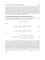
Fig. 5. The reciprocal of the condition number.
the robustness of the control system can be inferred. Fig. 5 shows the reciprocal condition
number for the case where the loudspeaker is symmetrically placed at a 1 m and 30
◦
relative
to the head center. The reciprocal condition number of the pressure control approaches to
zero, but the energy density control has the reciprocal condition numbers that are relatively
significant for entire frequencies. Thus, it can be said that the equalization in the energy
density field is more robust than the equalization in the pressure field.
Fig. 6. Simulation environments. (a) Configuration for the simulation of a multichannel
sound reproduction system. (b) Control points in the simulations. l
0

corresponds to the
center of the listener’s head.
0 2000 4000 6000 8000 10000 12000 14000 16000
0
0.5
Frequency (Hz)
V
min
/
V
max
0 2000 4000 6000 8000 10000 12000 14000 16000
0
0.5
1
Frequency (Hz)
V
min
/
V
max
(b) Energy density control
2
2
Q
Q

+
629
Robust Inverse Filter Design Based on Energy Density Control

4. Performance Evaluation
We present simulation results to validate energy density control. First, the robustness of
an inverse filtering for multichannel sound reproduction system is evaluated by simulating
the acoustic responses around the control points corresponding to the listener’s ears. The
performance of the robustness is objectively described in terms of the spatial extent of the
equalization zone.
4.1 S imulation result
In this simulation, we assumed a multichannel sound reproduction system consisting of four
sound sources (M
= 4) as shown in Fig. 6(a). Details of the control points are depicted in
Fig. 6(b). We assumed a free field radiation and the sampling frequency was 48 kHz. Impulse
responses from the loudspeakers to the control points were modeled using 256-tap FIR filters
(N
h
= 256), and equalization filters were designed using 256-tap FIR filters (N
w
= 256). The
conventional LS method was tried by jointly equalizing the acoustic pressure at l
1
, l
2
, l
3
,andl
4
points, and the energy density control was optimized only for the l
0
point. The delayed Dirac
delta function was used for the desired response, i.e., d
p,l

0
(n)=···= d
p,l
4
(n)=δ(n −n
0
).
Center The control point (cm)
frequency (0, 0) (0, 5) (2.5, 2.5) (5, 0) (5, 5)
500 Hz 0.06 -0.28 -0.13 -0.42 -0.28
1kHz 0.30 -1.39 -0.60 -1.91 -3.55
2kHz 1.26 -7.61 -2.76 -14.53 -10.25
Table 1. The error in dB for the pressure control system based on joint LS optimization at each
center frequency.
Center The control point (cm)
frequency (0, 0) (0, 5) (2.5, 2.5) (5, 0) (5, 5)
500 Hz 0.00 0.25 0.09 -0.21 0.03
1kHz 0.00 0.25 0.06 -0.95 -0.76
2kHz 0.00 0.25 -0.69 -4.50 -4.58
Table 2. The error in dB for the energy density control system at each center frequency.
We scanned the equalized responses in a 10 cm square region around the l
0
position, and
results are shown in Fig. 7. Note that only the upper right square region was evaluated due
to the symmetry. For the energy density control, velocity x and y were used. Velocity z was
not used. As evident in Fig. 7, the energy density control shows a lower error level than the
joint LS-based squared pressure control over the entire region of interest except at the points
corresponding to l
2
(2 cm,0 cm) and l

4
(0 cm,2 cm), where the control microphones for the
joint LS control were located.
Next, an equalization error was measured as the difference between the desired and actual
responses defined by
C
(dB)=10 log
⎧
⎪
⎪
⎨
⎪
⎪
⎩
ω
max
∑
ω=ω
min


D(ω) −
ˆ
D(ω)


2
ω
max
∑

ω=ω
min
|
D(
ω)
|
2
⎫
⎪
⎪
⎬
⎪
⎪
⎭
, (40)
630
Robust Control, Theory and Applications
Fig. 7. The spatial extent of equalization by controlling pressure based joint LS optimization
and energy density.
10
2
10
4
-10
0
10
(0cm, 5cm)
Response (dB)
10
2

10
4
-10
0
10
(1cm, 5cm)
10
2
10
4
-10
0
10
(2cm, 5cm)
10
2
10
4
-10
0
10
(3cm, 5cm)
10
2
10
4
-10
0
10
(4cm, 5cm)

10
2
10
4
-10
0
10
(5cm, 5cm)
10
2
10
4
-10
0
10
(0cm, 4cm)
Response (dB)
10
2
10
4
-10
0
10
(1cm, 4cm)
10
2
10
4
-10

0
10
(2cm, 4cm)
10
2
10
4
-10
0
10
(3cm, 4cm)
10
2
10
4
-10
0
10
(4cm, 4cm)
10
2
10
4
-10
0
10
(5cm, 4cm)
10
2
10

4
-10
0
10
(0cm, 3cm)
Response (dB)
10
2
10
4
-10
0
10
(1cm, 3cm)
10
2
10
4
-10
0
10
(2cm, 3cm)
10
2
10
4
-10
0
10
(3cm, 3cm)

10
2
10
4
-10
0
10
(4cm, 3cm)
10
2
10
4
-10
0
10
(5cm, 3cm)
(0cm 2cm)
(1cm 2cm)
(2cm 2cm)
(3cm 2cm)
(4cm 2cm)
(5cm 2cm)
Pressure control (LS)
Energy density control (LS)
10
2
10
4
-10
0

10
(0cm
,
2cm)
Response (dB)
10
2
10
4
-10
0
10
(1cm
,
2cm)
10
2
10
4
-10
0
10
(2cm
,
2cm)
10
2
10
4
-10

0
10
(3cm
,
2cm)
10
2
10
4
-10
0
10
(4cm
,
2cm)
10
2
10
4
-10
0
10
(5cm
,
2cm)
10
2
10
4
-10

0
10
(0cm, 1cm)
Response (dB)
10
2
10
4
-10
0
10
(1cm, 1cm)
10
2
10
4
-10
0
10
(2cm, 1cm)
10
2
10
4
-10
0
10
(3cm, 1cm)
10
2

10
4
-10
0
10
(4cm, 1cm)
10
2
10
4
-10
0
10
(5cm, 1cm)
10
2
10
4
-10
0
10
(0cm, 0cm)
Response (dB)
Frequency (Hz)
10
2
10
4
-10
0

10
(1cm, 0cm)
Frequency (Hz)
10
2
10
4
-10
0
10
(2cm, 0cm)
Frequency (Hz)
10
2
10
4
-10
0
10
(3cm, 0cm)
Frequency (Hz)
10
2
10
4
-10
0
10
(4cm, 0cm)
Frequency (Hz)

10
2
10
4
-10
0
10
(5cm, 0cm)
Frequency (Hz)
631
Robust Inverse Filter Design Based on Energy Density Control
where ω
min
and ω
max
denote the minimum and maximum frequency indices of interest,
respectively. In order to compare the robustness of equalization, we evaluated the pressure
level in the vicinity of the control points. The equalization errors are summarized in Tables
1 and 2. Results show that the energy density control has a significantly lower equalization
error than the joint LS-based squared pressure control, especially at 2 kHz where there are
7
∼ 10 dB differences.
Fig. 8. A three-dimensional plot of the error surface for the pressure control (left column) and
the energy density control (right column) at different center frequencies.
Finally, three-dimensional contour plots of the equalization errors are presented in Fig. 8.
Fig. 8(a) and (d) show both methods have similar equalization performance at 1 kHz due
to the relatively long wavelength. However, Figs. 8 (a), (b), and (c) indicate that the error
of the pressure control rapidly increases as the frequency increased. On the other hand,
the energy density control provides a more stable equalization zone, which implies that the
energy density control can overcome the observability problem to some extent. Thus, it can

be concluded that the energy density control system can provide a wider zone of equalization
than the pressure control system.
4.2 Implementation consideration
It should be mentioned that it is necessary to have the acoustic velocity components
to implement the energy density control system. It has been demonstrated that the
632
Robust Control, Theory and Applications
two-microphone approach yields performance which is comparable to that of ideal energy
density control in the field of the active noise control system Park & Sommerfeldt (1997). Thus,
it is expected that the energy density control being implemented using the two-microphone
approximation maintains the robustness of room equalization observed in the previous
simulations.
To examine this, we applied two microphone techniques, which were described in section 3.3,
to determine the acoustic velocity along an axis. By using Eq. (28), simulations were conducted
for the case of Δx
= 2cm to evaluate the performance of the two-sensor implementation.
Here, l
0
and l
2
are used for estimating the velocity component for x direction and l
0
and l
4
are used for estimating the velocity component for y direction; the velocity component for
z direction was not applied. The results obtained by using the ideal velocity signal and two
microphone technique are shown in Fig. 9. It can be concluded that the energy density system
employing the two microphone technique provides comparable performance to the control
system employing the ideal velocity sensor.
Fig. 9. The performance of the energy density control algorithm being implemented using the

two microphone technique.
5. Conclusion
In this chapter, a method of designing equalization filters based on acoustic energy density
was presented. In the proposed algorithm, the equalization filters are designed by minimizing
the difference between the desired and produced energy densities at the control points.
For the effective frequency range for the equalization, the energy density-based method
provides more robust performance than the conventional squared pressure-based method.
Theoretical analysis proves the robustness of the algorithm and simulation results showed
that the proposed energy density-based method provides more robust performance than the
conventional squared pressure-based method in terms of the spatial extent of the equalization
zone.
633
Robust Inverse Filter Design Based on Energy Density Control
6.References
Abe, K., Asano, F., Suzuki, Y. & Sone, T. (1997). Sound field reproduction by controlling the
transfer functions from the source to multiple points in close proximity, IEICE Trans.
Fundamentals E80-A(3): 574–581.
Elliott, S. J. & Nelson, P. A. (1989). Multiple-point equalization in a room using adaptive digital
filters, J. Audio Eng. Soc. 37(11): 899–907.
Gardner, W. G. (1997). Head-tracked 3-d audio using loudspeakers, Proc. IEEE Workshop on
Applications of Signal Processing to Audio and Acoustics, New Paltz, NY, USA.
Hodges, T., Nelson, P. A. & Elliot, S. J. (1990). The design of a precision digital integrator for
use in an active vibration control system, Mech. Syst. Sign. Process. 4(4): 345–353.
Kirkeby, O., Nelson, P. A., Hamada, H. & Orduna-Bustamante, F. (1998). Fast deconvolution
of multichannel systems using regularization, IEEE Trans. on Speech and Audio Process.
6(2): 189–195.
Mourjopoulos, J. (1994). Digital equalization of room acoustics, J. Audio Eng. Soc.
42(11): 884–900.
Mourjopoulos, J. & Paraskevas, M. (1991). Pole-zero modelling of room transfer functions, J.
Sound and Vib. 146: 281–302.

Nelson, P. A., Bustamante, F. O. & Hamada, H. (1995). Inverse filter design and equalization
zones in multichannel sound reproduction, IEEE Trans. on Speech and Audio Process.
3(3): 185–192.
Nelson, P. A., Hamada, H. & Elliott, S. J. (1992). Adaptive inverse filters for stereophonic
sound reproduction, IEEE Trans. on Signal Process. 40(7): 1621–1632.
Park, Y. C. & Sommerfeldt, S. D. (1997). Global control of broadband noise fields using energy
density control, J. Acoust. Soc. Am. 101: 350–359.
Parkins, J. W., Sommerfeldt, S. D. & Tichy, J. (2000). Narrowband and broadband active control
in an enclosure using the acoustic energy density, J. Acoust. Soc. Am. 108(1): 192–203.
Rao, H. I. K., Mathews, V. J. & Park, Y C. (2007). A minimax approach for the joint design
of acoustic crosstalk cancellation filters, IEEE Trans. on Audio, Speech and Language
Process. 15(8): 2287–2298.
Sommerfeldt, S. D. & Nashif, P. J. (1994). An adaptive filtered-x algorithm for energy-based
active control, J. Acoust. Soc. Am. 96(1): 300–306.
Sturm, J. F. (1999). Using sedumi 1.02, a matlab toolbox for optimization over symmetric
cones, Optim. Meth. Softw. 11-12: 625–653.
Toole, F. E. & Olive, S. E. (1988). The modification of timbre by resonances: Perception and
measurement, J. Audio Eng. Soc. 36: 122–141.
Ward, D. B. (2000). Joint least squares optimization for robust acoustic crosstalk cancellation,
IEEE Trans. on Speech and Audio Process. 8(2): 211–215.
Ward, D. B. & Elko, G. W. (1999). Effect of loudspeaker position on the robustness of acoustic
crosstalk cancellation, IEEE Signal Process. Lett. 6(5): 106–108.
634
Robust Control, Theory and Applications
30
Robust Control Approach for Combating the
Bullwhip Effect in Periodic-Review
Inventory Systems with Variable Lead-Time
Przemysław Ignaciuk and Andrzej Bartoszewicz
Institute of Automatic Control, Technical University of Łódź

Poland
1. Introduction
It is well known that cost-efficient management of production and goods distribution
systems in varying market conditions requires implementation of an appropriate inventory
control policy (Zipkin, 2000). Since the traditional approaches to inventory control, focused
mainly on the statistical analysis of long-term variables and (static) optimization performed
on averaged values of various cost components, are no longer sufficient in modern
production-inventory systems, new solutions are being proposed. In particular, due to the
resemblance of inventory management systems to engineering processes, the methods of
control theory are perceived as a viable alternative to the traditional approaches. A
summary of the initial control-theoretic proposals can be found in (Axsäter, 1985), whereas
more recent results are discussed in (Ortega & Lin, 2004) and (Sarimveis et al., 2008).
However, despite a considerable research effort, one of the utmost important, yet still
unresolved (Geary et al., 2006) problems observed in supply chain is the bullwhip effect,
which manifests itself as an amplification of demand variations in order quantities.
We consider an inventory setting in which the stock at a distribution center is used to fulfill
an unknown, time-varying demand imposed by customers and retailers. The stock is
replenished from a supplier which delivers goods with delay according to the orders
received from the distribution center. The design goal is to generate ordering decisions such
that the entire demand can be satisfied from the stock stored at the distribution center,
despite the latency in order procurement, referred to as lead-time delay. The latency may be
subject to significant fluctuations according to the goods availability at the supplier and
transportation time uncertainty. When demand is entirely fulfilled any cost associated with
backorders, lost sales, and unsatisfied customers is eliminated. Although a number of
researchers have recognized the need to explicitly consider the delay in the controller design
and stability analysis of inventory management systems, e.g. Hoberg et al. (2007),
robustness issues related to simultaneous delay and demand fluctuations remain to a large
extent unexplored (Dolgui & Prodhon, 2007). A few examples constitute the work of Boukas
et al. (2000), where an H
∞

-norm-based controller has been designed for a production-
inventory system with uncertain processing time and input delay, and Blanchini et al.
(2003), who concentrated on the stability analysis of a production system with uncertain
demand and process setup. Both papers are devoted to the control of manufacturing
Robust Control, Theory and Applications

636
systems, rather than optimization of goods flow in supply chain, and do not consider rate
smoothening as an explicit design goal. On the contrary, in this work, we focus on the
supply chain dynamics and provide formal methods for obtaining a smooth, non-oscillatory
ordering signal, what is imperative for reducing the bullwhip effect (Dejonckheere et al.,
2003).
From the control system perspective we may identify three decisive factors responsible for
poor dynamical performance of supply chains and the bullwhip effect: 1) abrupt order
changes in response to demand fluctuations, typical for the traditional order-up-to
inventory policies, as discussed in (Dejonckheere et al., 2003); 2) inherent delay between
placing of an order and shipment arrival at the distribution center which may span several
review periods; and finally, 3) unpredictable variations of lead-time delay. Therefore, to
avoid (or combat) the bullwhip effect, the designed policy should smoothly react to the
changes in market conditions, and generate order quantities which will not fluctuate
excessively in subsequent review intervals even though demand exhibits large and
unpredictable variations. This is achieved in this work by solving a dynamical optimization
problem with quadratic performance index (Anderson & Moore, 1989). Next, in order to
eliminate the negative influence of delay variations, a compensation technique is
incorporated into the basic algorithm operation together with a saturation block to explicitly
account for the supplier capacity limitations. It is shown that in the inventory system
governed by the proposed policy the stock level never exceeds the assigned warehouse
capacity, which means that the potential necessity for an expensive emergency storage
outside the company premises is eliminated. At the same time the stock is never depleted,
which implies the 100% service level. The controller demonstrates robustness to model

uncertainties and bounded external disturbance. The applied compensation mechanism
effectively throttles undesirable quantity fluctuations caused by lead-time changes and
information distortion thus counteracting the bullwhip effect.
2. Problem formulation
We consider an inventory system faced by an unknown, bounded, time-varying demand, in
which the stock is replenished with delay from a supply source. Such setting, illustrated in
Fig. 1, is frequently encountered in production-inventory systems where a common point
(distribution center), linked to a factory or external, strategic supplier, is used to provide
goods for another production stage or a distribution network. The task is to design a control
strategy which, on one hand, will minimize lost service opportunities (occurring when there
is insufficient stock at the distribution center to satisfy the current demand), and, on the
other hand, will ensure smooth flow of goods despite model uncertainties and external
disturbances. The principal obstacle in providing such control is the inherent delay between
placing of an order at the supplier and goods arrival at the center that may be subject to
significant fluctuations during the control process. Another factor which aggravates the
situation is a possible inconsistency of the received shipments with regard to the sequence of
orders. Indeed, it is not uncommon in practical situations to obtain the goods from an earlier
order after the shipment arrival from a more recent one. In addition, we may encounter
other types of disturbances affecting the replenishment process related to organizational
issues and quality of information (Zomerdijk & de Vries, 2003) (e.g. when a shipment arrives
on time but is registered in another review period, or when an incorrect order is issued from
Robust Control Approach for Combating the Bullwhip Effect in
Periodic-Review Inventory Systems with Variable Lead-Time

637
the distribution center). The time-varying latency of fulfilling of an order will be further
referred to as lead-time or lead-time delay.


Fig. 1. Inventory system with a strategic supplier

Fig. 2. System model
The schematic diagram of the analyzed periodic-review inventory system is depicted in
Fig. 2. The stock replenishment orders u are issued at regular time instants kT, where T is the
review period and k = 0, 1, 2, , on the basis of the on-hand stock (the current stock level in
the warehouse at the distribution center) y(kT), the target stock level y
d
, and the history of
previous orders. Each non-zero order placed at the supplier is realized with lead-time delay
L(k), assumed to be a multiple of the review period, i.e. L(k) = n(k)T, where n(k) and its
nominal value
n are positive integers satisfying

(
)
(
)
(
)
11nnk n
−
δ≤ ≤+δ (1)
and 0
≤
δ
< 1. Notice that (1) is the only constraint imposed on delay variations, which
means that within the indicated interval the actual delay of a shipment may accept any
statistical distribution. This implies that consecutive shipments sent by the supplier may
arrive out of order at the distribution center and concurrently with other shipments which

were sent earlier or afterwards. Since the presented model does not require stating the cause
of lead-time variations, neither specification of a particular function n(k) or its distribution, it
allows for conducting the robustness study in a broad spectrum of practical situations with
uncertain latency in delivering orders.
The imposed demand (the number of items requested from inventory in period k) is
modeled as an a priori unknown, bounded function of time d(kT),

(
)
max
0.dkT d≤≤ (2)
Notice that this definition of demand is quite general and it accounts for any standard
distribution typically analyzed in the considered problem. If there is a sufficient number of
items in the warehouse to satisfy the imposed demand, then the actually met demand h(kT)
Robust Control, Theory and Applications

638
(the number of items sold to customers or sent to retailers in the distribution network) will
be equal to the requested one. Otherwise, the imposed demand is satisfied only from the
arriving shipments, and additional demand is lost (we assume that the sales are not
backordered, and the excessive demand is equivalent to a missed business opportunity).
Thus, we may write

(
)
(
)
max
0.hkT dkT d≤≤≤
(3)

The dynamics of the on-hand stock y depends on the amount of arriving shipments u
R
(kT)
and on the satisfied demand h. Assuming that the warehouse is initially empty, i.e. y(kT) = 0
for k < 0, and the first order is placed at kT = 0, then for any kT ≥ 0 the stock level at the
distribution center may be calculated from the following equation

()
() () () ()
111 1
000 0
.
kkk k
R
jjj j
y
kT u
j
Th
j
Tu
j
TL
j
h
j
T
−−− −
=== =
⎡⎤

=−=−−
⎣⎦
∑∑∑ ∑
(4)
Let us introduce a function ξ(kT) = ξ
+
(kT) – ξ
–
(kT), where
•
ξ
+
(kT) represents the sum of these surplus items which arrive at the distribution center
by the time kT earlier than expected since their delay experienced in the neighborhood
of kT is smaller than the nominal one, and
•
ξ
–
(kT) denotes the sum of items which should have arrived by the time kT, but which
cannot reach the center due to the (instantaneous) delay greater than the nominal one.
Assuming that the order quantity is bounded by some positive value u
max
(e.g. the
maximum number of items the supplier can accumulate and send in one review period),
which is commonly encountered in practical systems, then on the basis of (1),

(
)
0maxmax
,

k
kT u L
≥
∀
ξ≤ξ=δ (5)
where
LnT= is the nominal lead-time. With this notation we can rewrite (4) in the
following way

()
()
()
()
11
00
.
kk
jj
y
kT u
j
nT kT h
j
T
−
−
==
⎡⎤
=−+ξ−
⎣⎦

∑∑
(6)
It is important to realize that because lead-time is bounded, it suffices to consider the effects
caused by its variations (represented by function ξ(·) in the model) only in the neighborhood
of kT implied by (1). Since the summing operation is commutative, all the previous
shipments, i.e. those arriving before (k –
n
δ
)T, can be added as if they had actually reached
the distribution center on time and this will not change the overall quantity of the received
items. In other words, delay variations of shipments acquired in the far past do not inflict
perturbation on the current stock.
The discussed model of inventory management system can also be presented in the state
space. The state-space realization facilitates adaptation of formal design techniques, and is
selected as a basis for the control law derivation described in detail in Section 3.
State-space representation
In order to proceed with a formal controller design we describe the discrete-time model of
the considered inventory system in the state space:
Robust Control Approach for Combating the Bullwhip Effect in
Periodic-Review Inventory Systems with Variable Lead-Time

639

(
)
(
)
(
)
(

)
(
)
() ()
12
1,
,
T
k T kT u kT h kT kT
ykT kT
⎡+ ⎤= + + +ξ
⎣⎦
=
xAxbvv
qx
(7)
where
x(kT) = [x
1
(kT) x
2
(kT) x
3
(kT) x
n
(kT)]
T
is the state vector with x
1
(kT) = y(kT)

representing the stock level in period k and the remaining state variables x
j
(kT) = u[(k –
n + j – 1)T] for any j = 2, , n equal to the delayed input signal u.
A is n × n state matrix, b,
v
1
, v
2
, and q are n × 1 vectors

12
110 0 0 1 1 1
001 0 0 0 0 0
, , , v , ,
000 1 0 0 0 0
000 0 1 0 0 0
−
⎡
⎤⎡⎤ ⎡⎤ ⎡⎤⎡⎤
⎢
⎥⎢⎥ ⎢⎥ ⎢⎥⎢⎥
⎢
⎥⎢⎥ ⎢⎥ ⎢⎥⎢⎥
⎢
⎥⎢⎥ ⎢⎥ ⎢⎥⎢⎥
=====
⎢
⎥⎢⎥ ⎢⎥ ⎢⎥⎢⎥
⎢

⎥⎢⎥ ⎢⎥ ⎢⎥⎢⎥
⎢
⎥⎢⎥ ⎢⎥ ⎢⎥⎢⎥
⎣
⎦⎣⎦ ⎣⎦ ⎣⎦⎣⎦
Abvq
…
…
    
…
…
(8)
and the system order
n = n + 1. For convenience of the further analysis, we can rewrite the
model in the alternative form

( ) () () () ()
() ()
() ()
() ()
112
23
1
1,
1,

1,
1.
nn
n

x k T x kT x kT h kT kT
xk T xkT
xkTxkT
xk T ukT
−
⎧
⎡+ ⎤= + − +ξ
⎣⎦
⎪
⎪
⎡+ ⎤=
⎣⎦
⎪
⎨
⎪
⎡+ ⎤=
⎣⎦
⎪
⎪
⎡+ ⎤=
⎣⎦
⎩

(9)
Relation (9) shows how the effects of delay are accounted for in the model by a special
choice of the state space in which the state variables contain the information about the most
recent order history. The desired system state is defined as

11
2

1
0
=,
0
0
dd
d
dn
dn
xx
x
x
x
−
⎡
⎤⎡ ⎤
⎢
⎥⎢ ⎥
⎢
⎥⎢ ⎥
⎢
⎥⎢ ⎥
=
⎢
⎥⎢ ⎥
⎢
⎥⎢ ⎥
⎢
⎥⎢ ⎥
⎣

⎦⎣ ⎦
d
x

(10)
where
x
d1
= y
d
denotes the demand value of the first state variable, i.e. the target stock level.
By choosing the desired state vector as
x
d
= [y
d
0 0 0]
T

we want the first state variable (on-hand stock) to reach the level y
d
, and to be kept at this
level in the steady-state. For this to take place all the state variables
x
2
x
n
should be zero
once
x

1
(kT) becomes equal to y
d
, precisely as dictated by (10).
In the next section, equations (7)–(10) describing the system behavior and interactions
among the principal system variables (ordering signal, on-hand stock level and imposed
demand) will be used to develop a discrete control strategy goverining the flow of goods
between the supplier and the distribution center.
Robust Control, Theory and Applications

640
3. Proposed inventory policy
In this section, we formulate a new inventory management policy and discuss its properties
related to handling the flow of goods. First, the nominal system is considered, and the
controller parameters are selected by solving a linear-quadratic (LQ) optimization problem.
Afterwards, the influence of perturbation is analyzed and an enhanced, nonlinear control
law is formulated which demonstrates robustness to delay and demand variations. The key
element in the improved controller structure is the compensator which reduces the effects
caused by delay fluctuations and information distortion.
3.1 Optimization problem
From the point of view of optimizing the system dynamics, we may state the aim of the
control action as bringing the currently available stock to the target level without excessive
control effort. Therefore, we seek for a control
u
opt
(kT), which minimizes the following cost
functional

() ( ) ( )
{

}
2
2
0
,
d
k
Ju u kT wy ykT
∞
=
=
+⎡ − ⎤
⎣
⎦
∑
(11)
where w is a positive constant applied to adjust the influence of the controller command and
the output variable on the cost functional value. Small w reduces excessive order quantities,
but lowers the controller dynamics. High w, in turn, implies fast tracking of the reference
stock level at the expense of large input signals. In the extreme case, when w → ∞, the term
y
d
– y(kT) prevails and the developed controller becomes a dead-beat scheme. From the
managerial point of view the application of a quadratic cost structure in the considered
problem of inventory control has similar effects as discussed in (Holt et al., 1960) in the
context of production planning. It allows for a satisfactory tradeoff between fast reaction to
the changes in market conditions (reflected in demand variations) and smoothness of
ordering decisions. As a result, the controller will track the target inventory level y
d
with

good dynamics, yet, at the same time, it will prevent rapid demand fluctuations from
propagating in supply chain. A huge advantage of our approach based on dynamical
optimization over the results proposed in the past is that the smoothness of ordering
decisions is ensured by the controller structure itself. This allows us to avoid signal filtering
and demand averaging, typically applied to decrease the degree of ordering variations in
supply chain, and thus to avoid errors and inaccuracies inherently implied by these
techniques.
Applying the standard framework proposed in (Zabczyk, 1974), to system (7)–(8), the
control u
opt
(kT) minimizing criterion (11) can be presented as

(
)
(
)
,
opt
ukT kTr
=
−+gx (12)
where

(
)
()
()
1
1
1

,
,
,
TT
TTT
TTT
d
r
w
y
−
−
−
=+
⎡⎤
=+ −
⎢⎥
⎣⎦
⎡⎤
=− + − −
⎢⎥
⎣⎦
n
nn
nn
gbKI bbK A
bKI bbK bb Ik
kAKIbbKbbIkq
(13)
Robust Control Approach for Combating the Bullwhip Effect in

Periodic-Review Inventory Systems with Variable Lead-Time

641
and semipositive, symmetric matrix K
n
×
n
, K
T
= K ≥ 0, is determined according to the
following Riccati equation

(
)
1
.
TT T
w
−
=+ +
n
KAKI bbK A qq (14)
Finding the parameters of the LQ optimal controller for the considered system with delay is
a challenging task, as it involves solving an nth order matrix Riccati equation. Nevertheless,
by applying the approach presented in (Ignaciuk & Bartoszewicz, 2010) we are able to solve
the problem analytically and obtain the control law in a closed form. Below we summarize
major steps of the derivation.
3.2 Solution to the optimization problem
We begin with the most general form of matrix K which can be presented as

11 12 13 1
12 22 23 2
13 23 33 3
0
123
.
n
n
n
nnn nn
kkk k
kkk k
kkk k
kkk k
⎡
⎤
⎢
⎥
⎢
⎥
⎢
⎥
=
⎢
⎥
⎢
⎥
⎢
⎥
⎣

⎦
K
…
…
…

…
(15)
In the first iteration, we place K
0
directly in (14), and after substituting matrix A and vector
b as defined by (8), we seek for similarities between the elements k
ij
on either side of the
equality sign in (14). In this way we find the relations among the first four elements in the
upper left corner of K: k
12
= k
22
= k
11
– w

(note that k
21
= k
12
since K is symmetric).
Consequently, after the first analytical iteration, we obtain the following form of K

11 11 13 1
11 11 23 2
13 23 33 3
1
123
.
n
n
n
nnnnn
kkwk k
kwkwk k
kkkk
kkk k
−
⎡
⎤
⎢
⎥
−−
⎢
⎥
⎢
⎥
=
⎢
⎥
⎢
⎥
⎢

⎥
⎣
⎦
K
…
…
…

…
(16)
Now we substitute K
1
given by (16) into the expression on the right hand side of (14) and
compare with its left hand side. This allows us to represent the elements k
i3
(i = 1, 2, 3) in
terms of k
11
as k
13
= k
23
= k
33
= k
11
– 2w. Concisely in matrix form we have

11 11 11 14 1
11 11 11 24 2

11 11 11 34 3
2
14 24 34 44 4
1234
2
2
222
.
n
n
n
n
nnnnnn
kkwkwk k
kwkwk wk k
kwkwkwk k
kkkkk
kkkkk
−−
⎡
⎤
⎢
⎥
−−−
⎢
⎥
⎢
⎥
−−−
=

⎢
⎥
⎢
⎥
⎢
⎥
⎢
⎥
⎢
⎥
⎣
⎦
K
…
…
…
…

…
(17)
We proceed with the substitutions until a general pattern is determined, i.e. until all the
elements of K can be expressed as functions of k
11
and the system order n. We get k
ij
= k
11
–
Robust Control, Theory and Applications

642
(j – 1)w for j ≥ i (the upper part of K) and k
ij
= k
11
– (i – 1)w for j < i (the lower part of K). In
matrix form

(
)
()
()
() () () ()
11 11 11 11
11 11 11 11
11 11 11 11
11 11 11 11
21
21
222 1.
111 1
kkwkwknw
kw kw k w k n w
kw kw kw knw
knwknwknw knw
⎡−−−−⎤
⎢⎥
−−− −−
⎢⎥
⎢⎥

=− − − −−
⎢⎥
⎢⎥
⎢⎥
−− −− −− −−
⎣⎦
K
…
…
…

…
(18)
If we substitute (18) into the right hand side of equation (14) and compare the first element
in the upper left corner of the matrices on either side of the equality sign, we get the
expression from which we can determine k
11
:

()
1
11 11
111.knw k n w
−
=
+−⎡ − − +⎤
⎣
⎦
(19)
Equation (19) has two roots

() ()
'"
11 11
21 4/2 and 21 4/2.kwnww kwnww
⎡⎤⎡⎤
=−−+ =−++
⎣⎦⎣⎦
(20)
Since det(
K) = w
n–1
[k
11
– (n – 1)w], only
() ()
"
11
21 4/2 1kwnww nw
⎡⎤
=−++≥−
⎣⎦

guarantees that
K is semipositive definite. Consequently, we get matrix K (18) with k
11
=
"
11
k .

This concludes the solution of the Riccati equation.
Having found
K, we evaluate g,

[]
()
{
}
1
11
111 11 1 1 .knw
−
=−⎡−−+⎤
⎣⎦
g …
(21)
Vector
k is determined by substituting matrix K given by (18) into the last equation in set
(13). We obtain

()
11 1 1
21,
T
dd d
kkwyk wy k n wy
=
⎡+ + +−⎤
⎣
⎦

k …
(22)
where

()
{
}
1
111
1.
d
kwynknw
−
=− +⎡ − − ⎤
⎣⎦
(23)
Then, using the second equation in set (13), and substituting (23), we calculate r,

(
)
() ()
1
11 11
1
.
11 1
d
d
kn wy
wy

r
knw knw
+
−
=− =
−− + −−
(24)
Finally, using (21) and (24), the optimal control u
opt
(kT) can be presented in the following
way:

() ()
()
()
()
11 11
1
1
1.
11 1
n
d
opt j
j
wy
ukT kTr xkT
knw knw
=
⎛⎞

=− + =− − +
⎜⎟
⎜⎟
−− + −−
⎝⎠
∑
gx
(25)
Robust Control Approach for Combating the Bullwhip Effect in
Periodic-Review Inventory Systems with Variable Lead-Time

643
Substituting
()
11
21 4/2kwnww
⎡⎤
=−++
⎣⎦
, we arrive at

() () ()
1
2
,
n
opt d j
j
ukT yxkT xkT
=

⎡
⎤
=α − −
⎢
⎥
⎢
⎥
⎣
⎦
∑
(26)
where the gain
(( 4) )/2ww wα= + − . From (9) the state variables x
j
(j = 2, 3, , n) may be
expressed in terms of the control signal generated at the previous n – 1 samples as

(
)
(
)
1.
j
xkT ukn j T
⎡
⎤
=−+−
⎣
⎦
(27)

Recall that we introduced the notation x
1
(kT) = y(kT). Then, substituting (27) into (26), we
obtain

() ()
()
1
,
k
opt d
jkn
ukT yykT ujT
−
=−
⎡
⎤
=α − −
⎢
⎥
⎢
⎥
⎣
⎦
∑
(28)
which completes the design of the inventory policy for the nominal system. The policy can
be interpreted in the following way: the quantity to be ordered in each period is
proportional to the difference between the target and the current stock level (y
d

– y(kT)),
decreased by the amount of open orders (the quantity already ordered at the supplier, but
which has not yet arrived at the warehouse due to lead-time delay). It is tuned in a
straightforward way by the choice of a single parameter α, i.e. smaller α implies more
dampening of demand variations (for a detailed discussion on the selection of α refer to
(Ignaciuk & Bartoszewicz, 2010)).
3.3 Stability analysis of the nominal system
The nominal discrete-time system is asymptotically stable if all the roots of the characteristic
polynomial of the closed-loop state matrix
A
c
= [I
n
– b(c
T
b)
–1
c
T
]A are located within the unit
circle on the z-plane. The roots of the polynomial

(
)
(
)
(
)
11
det 1 1 ,

nnn
zzzzz
−−
−
=+α− = ⎡−−α⎤
⎣
⎦
nc
IA (29)
are located inside the unit circle, if 0 < α < 2. Since for every n and for every w the gain
satisfies the condition 0 < α ≤ 1, the system is asymptotically stable. Moreover, since
irrespective of the value of the tuning coefficient w the roots of (29) remain on the
nonnegative real axis, no oscillations appear at the output. By changing w from 0 to ∞, the
nonzero pole moves towards the origin of the z-plane, which results in faster convergence to
the demand state. In the limit case when w = ∞, all the closed-loop poles are at the origin
ensuring the fastest achievable response in a discrete-time system offered by a dead-beat
scheme.
3.4 Robustness issues
The order calculation performed according to (28) is based on the nominal delay which
constitutes an estimate of the true (variable) lead-time set according to the contracting
agreement with the supplier. The controller designed for the nominal system is robust with
Robust Control, Theory and Applications

644
respect to demand fluctuations, yet may generate negative orders in the presence of lead-
time variations. In order to eliminate this deficiency and at the same time account for the
supplier capacity limitations, we introduce the following modification into the basic
algorithm

()

(
)
() ()
()
max
max max
0, if 0,
,if 0 ,
,if ,
kT
ukT kT kT u
ukTu
⎧ϕ<
⎪
=ϕ ≤ϕ ≤
⎨
⎪
ϕ>
⎩
(30)
where u
max
> d
max
is a constant denoting the maximum order quantity that can be provided
by the supplier in a single review period. Function φ(·) is defined as

() ()
() ()
()

11
0
.
kk
dR
jkn j
kT y y kT u jT u jT u jT L
−−
=− =
⎧
⎫
⎪
⎪
⎡
⎤
ϕ=α− − +ε − −
⎨
⎬
⎣
⎦
⎪
⎪
⎩⎭
∑∑
(31)
It consists of two elements:
•
LQ optimal controller as given by (28), and
•
delay variability compensator tuned by the coefficient ε ∈ [0, 1], which accumulates the

information about the differences between the number of items which actually arrived
at the distribution center and those which were expected to arrive.
3.5 Properties of the robust policy
The properties of the designed nonlinear policy (30)–(31) will be formulated as two
theorems and analyzed with respect to the most adverse conditions (the extreme
fluctuations of demand and delay). The first proposition shows how to adjust the warehouse
storage space to always accommodate the entire stock and in this way eliminate the risk of
(expensive) emergency storage outside the company premises. The second theorem states
that with an appropriately chosen target stock level there will be always goods in the
warehouse to meet the entire demand.
Theorem 1. If policy (30)–(31) is applied to system (7)–(8), then the stock level at the
distribution center is always upper-bounded, i.e.

(
)
(
)
max max max
0
1.
d
k
ykT y y u
≥
≤=+++εξ
∀
(32)
Proof. Based on (4), (5), and the definition of function ξ(·), the term compensating the effects
of delay variations in (31) satisfies the following relation

()
()
()
()
{}
()
()
11 1
00 0
.
kk k
R
jj j
u
j
Tu
j
TL u
j
TL
j
u
j
TL
j
TkT
−− −
== =
⎡⎤
⎡⎤

−−= − −−=ξ=ξ
⎣⎦
⎣⎦
∑∑ ∑
(33)
Therefore, we may rewrite function φ(·) as

() ()
()
()
1
.
k
d
jkn
kT y y kT u jT kT
−
=−
⎡
⎤
ϕ=α− − +εξ
⎢
⎥
⎢
⎥
⎣
⎦
∑
(34)
Robust Control Approach for Combating the Bullwhip Effect in

Periodic-Review Inventory Systems with Variable Lead-Time

645
It follows from the algorithm definition and the system initial conditions that the warehouse
at the distribution center is empty for any
(
)
1kn
≤
−δ . Consequently, it is sufficient to show
that the proposition holds for all
(
)
1kn>−δ. Let us consider some integer
(
)
1ln>−δ and
the value of φ(·) at instant lT. Two cases ought to be analyzed: the situation when φ(lT) ≥ 0,
and the circumstances when φ(lT) < 0.
Case 1. We investigate the situation when φ(lT) ≥ 0. Directly from (34), we get

() ()
()
1
.
l
d
jln
y
lT y lT u jT

−
=−
≤+εξ −
∑
(35)
Since u is always nonnegative, we have

(
)
(
)
.
d
y
lT y lT≤+εξ (36)
Moreover, since ξ(lT) ≤ ξ
max
, we obtain

(
)
max max
,
d
ylT y y≤+εξ ≤ (37)
which ends the first part of the proof.
Case 2. In the second part of the proof we analyze the situation when φ(lT) < 0. First, we
find the last instant l
1
T < lT when φ(·) was nonnegative. According to (34), φ(0) = αy

d
> 0, so
the moment l
1
T indeed exists, and the value of y(l
1
T) satisfies the inequality similar to (35),
i.e.

() ()
()
1
1
1
11
.
l
d
jl n
y
lT y lT u jT
−
=−
≤+εξ −
∑
(38)
The stock level at instant lT can be expressed as

() ( )
()

()
()
11
11
1
,
ln l
jl n jl
y
lT y l T u jT lT h jT
−− −
=− =
=+ +ξ−
∑∑
(39)
which after applying (38) leads to

() ( )
() ()
()
()
()()
() ()
1
11 1
11
1
11
1
11

1
.
l
ln l
d
jl n jl n jl
ln l
d
jl jl
y lT y l T u jT u jT lT h jT
ylTlT ujThjT
−
−− −
=− =− =
−− −
==
≤+εξ − + +ξ −
≤+εξ +ξ + −
∑∑ ∑
∑∑
(40)
The algorithm generated a nonzero quantity for the last time before lT at l
1
T, and this value
can be as large as u
max
. Consequently, the sum
()
()
1

1
1max
ln
jl
ujT ulT u
−−
=
=≤
∑
. From
inequalities (3) and the condition ξ(lT) ≤ ξ
max
we obtain the following stock estimate

(
)
(
)
(
)
(
)
11
max max max max
,
d
d
ylT y lT lT ulT
yuy
≤+εξ +ξ +

≤+εξ +ξ + =
(41)
Robust Control, Theory and Applications

646
which concludes the second part of the reasoning and completes the proof of Theorem 1. 
Theorem 1 states that the warehouse storage space is finite and never exceeds the level of
y
max
. This means that irrespective of the demand and delay variations the system output y(·)
is bounded, and the risk of costly emergency storage is eliminated. The second theorem,
formulated below, shows that with the appropriately selected target stock y
d
we can make
the on-hand stock positive, which guarantees the maximum service level in the considered
system with uncertain, variable delay.
Theorem 2. If policy (30)–(31) is applied to system (7)–(8), and the target stock level satisfies

(
)
(
)
max max
1/ 1 1 ,
d
yu n>+α+++εξ (42)
then for any k ≥ (1+δ)
n +T
max
/T, where T

max
= Ty
max
/(u
max
– d
max
), the stock level is strictly
positive.
Proof. The theorem assumption implies that we deal with time instants
(
)
max
1kT nT T≥+δ +
. Considering some
(
)
max
1/lnTT≥+δ+
and the value of signal φ(lT),
we may distinguish two cases: the situation when φ(lT) < u
max
, and the circumstances when
φ(lT) ≥ u
max
.
Case 1. First, we consider the situation when φ(lT) < u
max
. We obtain from (34)

()
()
()
1
max
.
l
d
jln
u
y
lT y u jT lT
−
=−
>− − +εξ
α
∑
(43)
The order quantity is always bounded by u
max
, which implies

(
)
(
)
max max
/.
d
y

lT y u u n lT>− α− +εξ (44)
Since ξ(·) ≥ – ξ
max
, we get

(
)
max max max
/.
d
ylT y u u n>− α− −εξ (45)
Using assumption (42), we get y(lT) > 0, which concludes the first part of the proof.
Case 2. In the second part of the proof we investigate the situation when φ(lT) ≥ u
max
. First,
we find the last period l
1
< l when function φ(·) was smaller than u
max
. It comes from
Theorem 1 that the stock level never exceeds the value of y
max
. Furthermore, the demand is
limited by d
max
. Thus, the maximum interval T
max
during which the controller may
continuously generate the maximum order quantity u
max

is determined as
T
max
= Ty
max
/ (u
max
– d
max
), and instant l
1
T does exist. Moreover, from the theorem
assumption we get l
1
T ≥ (1 + δ) nT, which means that by the time l
1
T the first shipment from
the supplier has already reached the distribution center, no matter the delay variation.
The value of φ(l
1
T) < u
max
. Thus, following similar reasoning as presented in (43)–(45), we
arrive at y(l
1
T) > 0 and

()
()
()

()
()
()
() ()
() ()
()
()
1
111
11
1
11
max
1
11 1
max
11
1
.
l
ln l
d
jl n jl n jl
ll l
d
jl jln jl
u
ylT y ujT lT ujT lT hjT
u
y

lT u lT u
j
Tu
j
TlT h
j
T
−
−− −
=− =− =
−− −
=+ =− =
>− − +εξ + +ξ −
α
=− +εξ + + − +ξ −
α
∑∑∑
∑∑ ∑
(46)
Robust Control Approach for Combating the Bullwhip Effect in
Periodic-Review Inventory Systems with Variable Lead-Time

647
Recall that l
1
T was the last instant before lT when the controller calculated a quantity smaller
than u
max
. This quantity, u(l
1

T), could be as low as zero. Afterwards, the algorithm generates
the maximum order and the first sum in (46) reduces to u
max
(l – 1 – l
1
). Moreover, since for
any k, u(kT) ≤ u
max
, the second sum is upper-bounded by u
max n
, which implies

() ( ) ( ) ()
()
1
1
max 1 max 1 max
/01 .
l
d
jl
y
lT
y
ulTullunlTh
j
T
−
=
>− α+εξ ++ −−− +ξ −

∑
(47)
According to (3), the realized demand satisfies 0 ≤ h(·) ≤ d
max
, hence

(
)
(
)
(
)
(
)
(
)
max max 1 max 1 max 1
/1 .
d
y
lT
y
uullunlTlTdll>− α+ −−− +εξ +ξ − − (48)
Since ξ(lT) ≥ – ξ
max
, we get

(
)
(

)
(
)
max max 1 max max max max 1
/1 .
d
y
lT
y
uullun dll>− α+ −−− −εξ −ξ − − (49)
Finally, using the theorem assumption (42), we may estimate the stock level at instant lT in
the following way

(
)
(
)
(
)
max max 1
.
y
lT u d l l>− −
(50)
Since l > l
1
, and by assumption u
max
> d
max

, we get y(lT) > 0. This completes the proof of
Theorem 2.

Remark. Theorem 2 defines the warehouse storage space which needs to be provided to
ensure the maximum service level. The required warehouse capacity is specified following
the worst-case uncertainty analysis (for an instructive insight how this methodology relates
to production-distribution systems see e.g. (Blanchini et. al., 2003) and (Sarimveis et al.,
2008)). Notice, however, that the value given in (42) scales linearly with the maximum order
quantity related to demand by the inequality u
max
> d
max
. Therefore, in the situation when
the mean demand differs significantly from the maximum one, it may be convenient to
substitute u
max
with some positive d
L
< d
max
< u
max
. In such a case the 100% service level is no
longer ensured, yet the average stock level, and as a consequence the holding costs, will be
reduced.
4. Numerical example
We verify the properties of the nonlinear inventory policy (30)–(31) proposed in this work in
a series of simulation tests. The system parameters are chosen in the following way: review
period T = 1 day, nominal lead-time
LnT

=
= 8 days, tolerance of delay variation δ = 0.25,
the maximum daily demand at the distribution center d
max
= 50 items, and the maximum
order quantity u
max
= 55 items. In order to provide fast response yet with a smooth ordering
signal, the controller gain should not exceed 0.618, which corresponds to the balanced
optimziation case with w = 1. Since, additionally, we should account for ordering
oscillations caused by delay changes, in the tests the gain is adjusted to α(w) = α(0.5) = 0.5.
We consider two scenarios reflecting the most common market situations.
Scenario 1. In the first series of simulations we test the controller performance in response to
the demand pattern illustrated in Fig. 3, which shows a trend in the demand with abrupt
seasonal changes. It is assumed that lead-time fluctuates according to
Robust Control, Theory and Applications

648

(
)
(
)
(
)
1 sin 2 / 1 0.25sin /4 8 ,Lk kT n nT k
⎢
⎥⎢ ⎥
=⎡+δ π ⎤ =⎡+ π ⎤
⎣⎦⎣⎦

⎣
⎦⎣ ⎦
(51)
where ⎣f⎦ denotes the integer part of f. The actual delay in procurring orders is illustrated in
Fig. 4.


Fig. 3. Market demand – seasonal trend


Fig. 4. Lead-time delay
In order to elaborate on the adverse effects of delay variations, and assess the quality of the
proposed compensation mechanism, we run two tests. In the first one (curve (a) in the
graphs), we show the controller performance with compensation turned off, i.e. with
ε
= 0,
and in the seond test, we consider the case of a full compensation in action with
ε
set equal
to 1 (curve (b) in the graphs). The target stock level y
d
is adjusted according to the
guideliness provided by Theorem 2 so that the maximum service level is obtained, and the
storage space y
max
is reserved according to the condition stipulated in Theorem 1. The actual
values used in the simulations are summarized in Table 1.
The test results are shown in Figs. 5–7: the ordering signal generated by the controller in
Fig. 5, the received orders in Fig. 6, and the resultant on-hand stock in Fig. 7. It is clear from
the graphs that the proposed controller quickly responds to the sudden changes in the

demand trend. Moreover, the stock does not increase beyond the warehouse capacity, and it
never drops to zero after the initial phase which implies the 100% service level. If we
compare the curves representing the case of a full compensation (b) and the case of the
Robust Control Approach for Combating the Bullwhip Effect in
Periodic-Review Inventory Systems with Variable Lead-Time

649
compensation turned-off (a) in Figs. 5 and 7, we can notice that the proposed compensation
mechanism eliminates the oscillations of the control signal originating from delay variations.
This allows for smooth reaction to the changes in market trend, and an ordering signal
which is easy to follow by the supplier. We can learn from Fig. 7 that the obtained smooth
ordering signal also permits reducing the on-hand stock while keeping it positive. This
means that the maximum service level is achieved, but with decreased holding costs.

Compensation
{on/off}
Target stock
y
d
[items]
Storage space
y
max
[items]
off:
ε
= 0
720 > 715 885
on:
ε

= 1
830 > 825 1105
Table 1. Controller parameters in Scenario 1


Fig. 5. Generated orders


Fig. 6. Received shipments
Scenario 2. In the second scenario, we investigate the controller behavior in the presence of
highly variable stochastic demand. Function d(·) following the normal distribution with
mean d
μ
= 25 items and standard deviation d
δ
= 25 items, D
norm
(25, 25), is illustrated in Fig. 8.

Robust Control, Theory and Applications

650

Fig. 7. On-hand stock
Since the mean demand in the stochastic pattern significantly differs from the maximum
value, we adjust the target stock according to (42) with u
max
> d
max
replaced by d

μ
= 25 items.
This results in y
d
= 375 items (with
ε
= 1). Although it is no longer guaranteed to satisfy all of
the customer demand (the service level decreases to 98%), the holding costs are nearly
halved. For the purpose of comparison we also run the tests for a classical order-up-to
(OUT) policy (order up to a target value y
OUT
if the total stock – equal to the on-hand stock
plus open orders – drops below y
OUT
). In order to compare the controllers in a fair way, we
apply the same compensation mechanism for the OUT policy as is used for our, LQ-based
scheme. We also reduce the value of the target stock level for the OUT policy y
OUT
setting
α
= 1 in (42). The controller parameters actually used in the test are grouped in Table 2.
Lead-time is assumed to follow the normal distribution D
norm
(8 days, 2 days). The actual
delay in procurring orders is illustrated in Fig. 9.


Policy
Target
stock

y
d
| y
OUT
[items]
Storage space
y
max
[items]
LQ-based 375 500
OUT 350 475
Table 2. Controller parameters in Scenario 2
The orders generated by both policies are shown in Fig. 10, the received shipments in
Fig. 11, and the on-hand stock in Fig. 12. It is evident from the plots that in contrast to the
OUT policy (a), our scheme (b) successfully dampens demand fluctuations at the very first
stage of supply chain, and it results in a smaller on-hand stock. Performing statistical
analysis we obtain 261 items
2
order variance for the OUT policy and 99 items
2
for our
controller. Consequently, according to the most popular (Miragliota, 2006) measure of the
bullwhip effect proposed by Chen et al. (2000), which is the ratio of variances of orders and
demand, we obtain for our scheme 0.44, which corresponds to 2.27 attenuation of demand
variations. The ratio of variances for the OUT policy equals 1.16 > 1 which implies amplified
variations and the bullwhip effect. This clearly shows the benefits of application of formal
control concepts, in particular dynamical optimization and disturbance compensation, in
alleviating the adverse effects of uncertainties in supply chain.
Robust Control Approach for Combating the Bullwhip Effect in
Periodic-Review Inventory Systems with Variable Lead-Time

651

Fig. 8. Market demand following the normal distribution with mean and standard deviation
equal to 25 items


Fig. 9. Lead-time delay following the normal distribution with mean 8 days and standard
deviation 2 days


Fig. 10. Generated orders