Wave Propagation Part 16 ppt
Bạn đang xem bản rút gọn của tài liệu. Xem và tải ngay bản đầy đủ của tài liệu tại đây (1.58 MB, 35 trang )
12
,
ϕ
π
λ=λ =± . The physical analog of the point at infinity is the dihedral corner reflector.
All points of the imaginary axis correspond to the objects with
{
}
Re 0
μ
=
, i.e.
12
λ=λ. In
this case, the points laying on the positive imaginary semi-axis, present radar objects which
are characterized by the phase shift 0
ϕ
> , while the negative imaginary semi-axis
Fig. 5. The complex plane of radar objects
(
{
}
Im 0
μ
<
) depicts the objects with 0
ϕ
<
. The points j
±
present the objects having
()
/2
ϕπ
=± phase shift. All real axis’s points of the complex
μ
−plane correspond to the
objects with zero phase shift
0;
ϕ
=
(i. e.
{
}
Im 0
μ
=
). However, the given case is
complicated by the fact that the object, which corresponds to the point at infinity, is the
dihedral reflector. This contradiction can be solved, considering the equality
sin 0
ϕ
= both
for
0;
ϕ
= and ;
ϕ
π
=
cases. Then the points of the real axis of the complex
μ
−plane must
be determined with the use of the conditions ( cos0 1, cos 1
π
=
=− ) as
{}
(
)
(
)
12
Re / 2
ϕ
μ
=λ−λ λ+λ+ λλ
C . Thus, into the interval
{
}
{
}
Re 0; Re 1
μμ
=
=
the
value
2
λ
reduces from
12
λ
λ
=
in the origin up to
2
0
λ
=
in the point
{
}
Re 1
μ
=
(horizontal
oriented object). This point depicts the “degenerated” radar object (long linear object, dipole,
i.e. polarizer). The phase shift in the point has an undefined value. It changes spasmodically
by
π
when passing the point
{
}
Re 1
μ
=
. Then, the value
2
λ
increases from
2
0
λ
= (in the
point
{
}
Re 1
μ
=
) up to
12
λ
λ
=
(the point at infinity). In this case, the phase shift along the
ray
{
}
{
}
Re 1; Re
μμ
==∞
equals to
π
. The similar analysis can be made with respect to the
negative semi-axis
{
}
Re
μ
. Thus, the complex
μ
−plane has the properties equivalent to the
properties of the circular complex plane . However, at that time when the circular complex
plane presents the polarization properties of electromagnetic waves, the complex
μ
−plane
is intended for presentation of the invariant polarization parameters of the radar objects
scattering matrix.
Analyzing the similarity, which exists between the
μ
−plane and the circular complex plane,
we can conclude that it is expedient to choose the circular basis as the basis for presenting
the radiated and scattered waves. The scattering matrix (8) in the circular basis can be found
in the form (Tatarinov at al, 2006)
O
μ
Im
μ
μ
μ
ar
g
μ
j
+
j
−
1
−
1
+
Δ
ϕ=0
Δ
ϕ=π
Δ
ϕ=0
Δ
ϕ=π
(
)
()
{
}
(
)
() ()
()
{}
12 12
12 12
exp 2 / 2
0,5
exp 2 / 2
RL
jl
j
Sj
j
λλ βπ λλ
λλ λλ βπ
−− +
=
+−−−
. (13)
Change of the rotation direction under backscattering is also considered in this expression.
Let us present the radiated wave in the circular basis
(
)
,
RL
ee
G
G
. The circular polarization
ratio for this wave can be written as
/
RL
RRL
PEE=
. Then, the circular polarization ratio for
the scattered wave will have the form
[]
{
}
[]
{
}
1/2//2
RL RL RL
SRR
PPP
μβπ μβπ
=+ +
jj. (14)
It is possible to set the specific polarization state of the radiated wave, when polarization
ratio of the scattered wave will have an unique form. So, if
RL
R
P
=
∞
, (right circular polarized
wave ) then we can rewrite the expression (14) in the form
1exp{-(2-/2)}
lim exp{ [ ) /2]}.
exp{- ( 2 - /2)}
RL
RL
R
S
RL
R
P
jP
Pj
RL
jP
R
μβπ
βμπ
μβπ
→∞
+
=−−−
+
(15)
If 0
θ
= , then we get
[
]
exp{ ) /2 }
RL
S
Pj
μμπ
=− +
. (16a)
Using the Jones vector
RL
E
G
we can find the circular polarization ratio in the form
(
)
(
)
{
}
tan / 4 exp 2 /2 .
RL
Pi
απ βπ
=+ −−
(16b)
Here
α
is an ellipticity angle and
β
is an orientation angle of polarization ellipse.
The comparison of expressions (16a, b)shows that the measured module of the circular
polarization ratio of the scattered wave (when the radiated wave has right circular
polarization) is equal to the complex degree polarization anisotropy (CDPA) module
RL
S
P
α
πμ
. (17)
The argument of the
RL
S
P
(for the case 0
θ
=
) can be presented as
{
}
ar
g
/2 2 /2
μπ βπ
+=−+
or
{
}
ar
g
2
μ
β
=−
. The last expression demonstrates that the
value of CDPA argument determines the orientation of the polarization ellipse in the
eigencoordinates system of the scattering object. If 0
θ
≠
, then the polarization ellipse will
be rotated additionally an angle of
2
β
. The correspondence between the circular complex
plane and the Riemann sphere, having unit diameter, was analyzed in details in (Tatarinov
at al, 2006) with the use of the stereographic projection equations, which are connecting on-
to-one the circular complex plane points
Re Im
RL RL RL
PP
j
P=+
with Cartesian coordinates
123
, , XXX of the point S , laying on the Riemann sphere surface. The transition from the
circular complex plane to the Poincare sphere , having unit radius, can be realized with the
use the modified stereographic projection equations
2
2Re / 1 ,
RL RL
XP P
⎛⎞
=+
⎜⎟
⎝⎠
2
2Im / 1 ,
RL RL
YP P
⎛⎞
=+
⎜⎟
⎝⎠
22
2/1 0,5.
RL RL
ZP P
⎧
⎫
⎛⎞
=+−
⎨
⎬
⎜⎟
⎝⎠
⎩⎭
Using these equations we can connect the complex
μ
-plane of radar objects with the sphere
of unit radius(fig. 6).
Fig. 6. Polarization sphere of radar objects
We will assume that the axes
12
, SS
G
G
of the three-dimensional space
123
, , SSS are
coinciding with real and imaginary axes
{
}
{
}
Re , Im
μ
μ
of the radar objects complex plane
Re Imj
μ
μμ
=+
respectively. In accordance with stated above, all point of this
T
S
-sphere
will be connected one-to-one with corresponding points of radar objects complex
μ
-plane.
Let us consider now that a radar object is defined on the
μ
-plane by the point
TR I
j
μ
μμ
=+
. Then we will connect the point
T
μ
with the sphere north pole by the line,
which crosses the sphere surface at point
T
S
. The projections
123
, ,
TTT
SSS of the point
T
S to
the axes
123
, , SSS
will be defined to modified stereographic projection equation. It is not
difficult to see that these values are satisfying to the unit sphere equation
(
)
(
)
(
)
222
123
1
TTT
SSS++=
.
Thus, all points of the complex plane of radar objects are corresponding one-to-one to points
of the sphere
T
S . We will name this sphere as the unit sphere of radar object .
2.3 Scattering operator of distributed radar object and its factorization
Let us to write now the Jones vector of the field scattered by the RDRO in the form
()
{}
{} {}
{} {}
11 12
0
1
11
0
0
0
2
21 22
11
exp 2 exp 2
exp 2
,
4
exp 2 exp 2
NN
MMMM
MM
S
NN
MMMM
MM
Sjk Sjk
E
jkR
Ek
R
E
Sjk Sjk
ηη
δϕ
π
ηη
==
Σ
==
−
=
∑∑
∑∑
, (18)
where
m
mm
xz
ηδϕ
′′
=+ and matrix
3
S
1
SRe
⇔
μ
2
SIm
⇔
μ
T
μ
Im
T
μ
Re
T
μ
A
0
T
S
T
1
S
T
2
S
T
3
S
()
{}
{} {}
{} {}
11 12
11
0
0
21 22
11
exp 2 exp 2
exp 2
,
4
exp 2 exp 2
NN
MMMM
MM
jl
NN
MMMM
MM
Sjk Sjk
jkR
Sk
R
Sjk Sjk
ηη
δϕ
π
ηη
==
Σ
==
−
=
∑∑
∑∑
(19)
is scattering operator, which includes space, polarization and frequency property of random
distributed radar object. It follows from the expression (19) that all elements of the RDRO
scattering operator
()
,
jl
Sk
δ
ϕ
Σ
are the function of two variables. These variables are as the
wave vector absolutely value and positional angle
ϕ
. A dependence from the wave vector
absolutely value is the frequency dependence, as far as for a media having the refraction
parameter 1n = the wave vector has the form 2 / /
kc
π
λω
=
= , where c is light velocity
and
2
f
ω
π
= . It is necessary to note here that scattered field polarization parameters at the
scattering by one-point radar object are independent both from positional angle and
frequency. For analysis of polarization-angular and polarization-frequency dependences of
the field at the scattering by the RDRO we write the exponential function
[
]
{
}
exp 2 2
MM
jkx kz
δϕ
′′
−+
that has been included into the operator (19) elements. The index
of this function is originated by the existence both angular and frequency dependences of
the field scattered by the RDRO. We will rewrite this index for its analysis:
(
)
,2 2
M
MM
f
kkxkz
δϕ δϕ
′
′
=+. (20)
Let’s us assume that the initial wave is quasimonochromatic (
0
/
ω
ω
Δ
<< 1) and that radar
radiation frequency arbitrary changes are not disturbing this condition. We can write the
wave vector
k absolutely value in the form
(
)
(
)
0
//kc c
ωωω
==+Δ, (21)
where
0
ω
is a mean constant frequency of radar radiation, and
ω
Δ
is a variable part
originated by radar radiation frequency change or frequency modulation. The substitution
of the expression (21) in the expression (20) give us
(
)
(
)
(
)
()()( )
00
00
, 2 / 2 /
2/2/2 /
MmM
MMMM
f
kxczc
xc zcx z c
δϕ ω ω δϕ ω ω
ωδϕ ω δϕω ω
′
′
⎡
⎤⎡ ⎤
=
+Δ + +Δ =
⎣
⎦⎣ ⎦
′′′′
=++Δ+Δ
. (22)
As far as the value
0
ω
is constant, then from all items of the expression (22) only the value
2/
m
xc
δ
ϕω
′
Δ
is depending simultaneously both on variable positional angle
δ
ϕ
and on
frequency variable
ω
Δ
. However, it is not difficult to see that the inequality
(
)
(
)
2/2/
MM
xczc
δϕ ω ω
′′
Δ<<Δ
(23)
is correct under the condition
1
Rad
δ
ϕ
<
<
(i.e. 10
δϕ
≤
D
). Taking into account this inequality,
we can neglect by the value
2/
M
xc
δ
ϕω
′
Δ
in the equation (23) and then we can rewrite it in
the form
(
)
00
, , 2
MMM
fk kx t
δ
ϕω δϕ ω
′
′
Δ≈ +
, (24)
where
0
ω
ωω
=+Δ, 2/
MM
tzc
′
′
=
. Thus, the angular and frequency variables in the
expression (24) are separated. It is so-called factorization operation. The value
M
t is a
doubled time interval, which is necessary for initial wave passage of a distance, which is a
projection of segment
M
z on the OZ
′
axis, i.e. on the propagation direction of radar initial
wave. This analysis shows that the scattered field polarization parameters frequency
dependence at the scattering by the RCRO is defined by the projections of the scattering
centers co-ordinates on the
OZ
′
axis, which is coinciding with the radar initial wave
propagation direction. In other words, a frequency dependence is defined by the RCRO
extension along the initial wave propagation direction. It follows simultaneously from the
equation (33) that the scattered field polarization-angular dependence on the mean
frequency
0
ω
is defined by the values
m
x
′
collection. These values are projections of
scattering centers positions on the
OX
′
axis that is perpendicular to radar initial wave
propagation direction. So, an extension of the RCRO along the
OX
′
axis is originated a
polarization-angular dependence of field polarization parameters at the scattering by a
RCRO.
3. Angular response function of a distributed object and its basic forms
Taking into account the results of subsection 2.3 we can now consider separately the
polarization-angular and polarization-frequency forms of a distributed radar object
responses on unit action, having circular polarization.
In accordance with the mentioned results the polarization-angular response of a complex
object at mean frequency
0
ω
is determined by extension of the object along the axis OX
′
,
that is perpendicular to direction of incident wave propagation’s. Taking into account the
expression (18) we can write the scattering operator (28) of the distributed radar object for
the circular polarization basis in the form
()
{}
() ()
() ()
,,
11 0 12 0
00
,
0
,,
0
21 0 22 0
, ,
exp 2
,
4
, ,
RL RL
RL
jl
RL RL
Sk Sk
jkR
Sk
R
Sk Sk
δ
ϕδϕ
δϕ
π
δ
ϕδϕ
ΣΣ
Σ
ΣΣ
−
=
, (25)
Where
()
[]
{}
,
11 0 0 3
1
,exp2
N
RL M
MM
M
Sk jkx
δϕ δϕ β
Σ
=
′
=Δ −
∑
;
()
[]
{}
,
22 0 0 1
1
,exp2
N
rl m
mm
m
Sk jkx
δϕ β
Σ
=
′
=− Δ −
∑
;
() ()
[]
{}
,,
12 0 21 0 0 2
1
,, exp2
N
rl rl m
mm
m
Sk Sk j jkx
δϕ δϕ δϕ β
ΣΣ
=
′
==Σ −
∑
.
Here
2
arg 2
M
M
M
kz
β
′
=Σ−
;
1
arg 2 2
M
M
MM
kz
βθ
′
=Δ− −
;
2
arg 2
M
M
M
kz
β
′
=Σ−
;
3
arg 2 2
M
M
MM
kz
βθ
′
=Δ+ −
and values
MMM
12 1 2
Δ =λ -λ ,
M
MM
λ
λ
Σ= +
are the difference and
union of
M
th− elementary scatterers eigen values . If the Jones vector of the incident wave
is right circular polarized, we can write for the circular Jones vector of the wave, scattered
by a distributed radar object in the form
()
{}
[]
{}
[]
{}
2
1
00
,
0
0
1
1
exp
exp 2
,
4
exp
N
M
MM
M
RL
S
N
M
MM
M
jj
jkR
Ek
R
j
δϕ β
δϕ
π
δϕ β
=
Σ
=
−Σ Ω−
−
=
ΔΩ−
∑
∑
G
. (26)
We are using here the notion of spatial frequencies
0
2
M
M
kx
′
Ω
= (Kobak, 1975), (Tatarinov et
al, 2006) that allows us to consider the elements of the Jones vector (26) as the sum of a large
number harmonic oscillations. The moving coordinate of these oscillation is the variable
positional angle
δ
ϕ
. The frequencies of these oscillations are determined by projections of
the coordinates of scattering centers
M
T on the axis OX
′
.
Amplitudes of oscillations are the values
M
Σ
,
M
Δ
can be characterized by the Rayleigh
distribution (Potekchin et al, 1966) and the random initial phases
1
M
β
,
2m
β
may have the
uniform distribution into the interval 0 2
π
÷
. Stochastic values of the spatial frequencies
M
Ω may have the uniform distribution in the interval
M
IN MAX
Ω
÷Ω . This interval
correspond to domain of definition
M
IN MAX
xx
′
′
÷
along the OX
′
axis. Thus, we can consider
the sum (26) as a complex stochastic function of the moving coordinate
δ
ϕ
.
The circular polarization ratio for mean frequency
0
ω
we can write using elements of Jones
vector (26) in this case will have the form
()
[]
{}
[]
{}
012
11
, exp / exp
NN
RL M M
SMMMM
MM
Pk j j j
δϕ δϕ β δϕ β
==
=Δ Ω− Σ Ω−
∑∑
. (27)
This ratio represents an angular distribution of the polarization parameters of an RCRO and
it is the polarization-angular response function of a random distributed radar object on the
unit action, having the form of a circular polarized wave.
Polarization-angular response function (27) is a generalization of the point object response
(16a) on the unit action, having the form of a circular polarized wave. Both the polarization
properties of scatterers, and geometrical parameters of a random distributed radar object are
represented into the polarization-angular response (27). We will transform every item of the
numerator of (27) in the following form
[]
{}
(
)
[]
{}
[]
{}
11
1
exp / exp
exp
MMMM
MM MM
MM
MM
jj
j
δϕ β δϕ β
μδϕβ
Δ Ω−=ΣΔΣ Ω−=
=Σ Ω −
Here the values
M
μ
are determined by expression (10) and represent modules of
elementary scatterer’s
M
T
complex degree polarization anisotropy. The values
M
μ
, that
are describing the polarization properties of elementary reflectors of an RDRO, make up a
general expression by using the weight factors
()()
0,5
22
12 12
2cos
MM M MM
M
λλ λλϕ
⎡
⎤
Σ= + + Δ
⎢
⎥
⎣
⎦
.
Taking into account this fact, we can find
() ()
{}
()
{}
012
11
, exp / exp
NN
RL M M M
SMMMM
MM
Pk j j j
δϕ μ δϕ β δϕ β
==
=Σ Ω− Σ Ω−
∑∑
. (28)
The weight factors
m
Σ
are connected with the radar cross sections of elementary scatterers.
The angular distribution of the polarization ratio (28) completely describes the polarization
structure of the field, scattered by a complex object
() () ()
{
}
00 0
, tan , exp 2 ,
4
RL
S
Pk k j k
π
δ
ϕαδϕ βδϕ
⎡⎤
=+
⎣⎦
. (29)
Here values
(
)
0
, k
α
δϕ
and
(
)
0
, k
β
δϕ
are angular distributions both of the ellipticity angle
and the orientation angle of the polarization ellipse of the scattered field.
Existing measurement methods allow us to carry out direct measurements of the module of
a polarization ratio. Thus, we have the possibility for the direct measurements of ellipticity
angle of the scattered wave. The measurement of the orientation needs indirect methods.
First of all we shall consider the opportunity of the characteristics of an ellipticity angle in
the analysis of wave polarization, scattered by random distributed objects. We will use all
forms of complex radar object polarization-angular response, which are different functions
of an ellipticity angle. The following parameters are connected with an ellipticity angle
value:
-
The value
()
()
0
tan / 4 ,
RL
Pk
α
πδϕ
+=
, determined in the interval
(
)
0tan /4
απ
≤+≤∞;
-
The coefficient of ellipticity
(
)
0
, tanKk
δ
ϕα
=
, determined in the interval
1tan 1
α
−≤ ≤ . This coefficient is connected with the module of circular polarization
ratio
RL
P
by
()
(
)
(
)
(
)
(
)
0
, tan 1 / 1 tan 1 / tan 1
44
RL RL
Kk P P
ππ
δϕ α α α
⎡⎤
⎡
⎤⎡ ⎤
== − += +− ++
⎢⎥
⎣
⎦⎣ ⎦
⎣⎦
; (30)
-
-The third normalized Stokes parameter
3
sin 2S
α
=
, determined in the
interval
3
11S−≤ ≤ .
This parameter is connected with the square of the circular polarization ratio module as
() () () ()
22
30 0 0 0
, sin2 , , 1 / , 1
RL RL
SS
Sk k P k P k
δϕ α δϕ δϕ δϕ
⎡
⎤⎡ ⎤
=
=− +
⎢
⎥⎢ ⎥
⎣
⎦⎣ ⎦
. (31a)
The Stokes parameter
3
S
and the ellipticity coefficient
K
are connected by the expression
()
(
)
2
3
sin 2 sin 2arctan 2 / 1SKKK
α
== = +. (31b)
The inverse function
(
)
3
KS is the solution of the equation
2
33
20SK K S
−
+=. We will
choose the solution
()
(
)
2
333
11 /KS S S=− −
from two versions
(
)
2
1/2 3 3
11 /KSS=± −
. It
follows from conformity
1K
=
− ,
3
1S
=
− ; 0K
=
,
3
0S
=
; 1K
=
,
3
1S
=
that only solution
(4c) remains. Thus, we can use the initial polarization-angular response
() ()
00
, tan , /4
rl
S
Pk k
δϕ α δϕ π
⎡
⎤
=+
⎣
⎦
and two other forms of responses -
(
)
(
)
00
, tan , Kk k
δ
ϕαδϕ
⎡⎤
=
⎣⎦
and
(
)
(
)
30 0
, sin2 , Sk k
δ
ϕαδϕ
= .
-1
-0,5
0
0,5
1
1 13 25 37 49 61 73 85 97 109 121 133 145 157 169 181 193
Fig. 7. The experimental realization of polarization- angular response function
(
)
3
S
δ
ϕ
For example, the experimental realization, having the form of narrow-band angular
dependence
(
)
3
S
δ
ϕ
has shown on the Fig. 7. The angular extension of this experimental
realization is
0
20± at the observation to radar object board . The samples of polarization-
angular response function are following with the angular interval
0
0,2 .
4. An emergence principle and polarization coherence notion
The analysis of an electromagnetic field polarization properties at the scattering by space
distributed radar object is closely connected with two key problems. The first problem is the
influence of separated scatterers space diversity on scattered field polarization. The second
key problem of polarization properties investigation at the scattering by distributed radar
object is connected with scattered field polarization properties definition on the base of the
emergence principle with the use of possible relations between complex radar object parts
polarization properties.
4.1 An emergence principle and space frequency notion for a simplest distributed
object. polarization proximity and polarization distance
Let us to define a field, scattered by RDO using the Stratton-Chu integral (1), which
allows us to represent this field as the union of waves scattered by elementary scatterers
(“bright” or “brilliant” points), forming complex object. For the case when every elementary
scatterer is characterizing by its scattering matrix
()
; , l 1, 2
M
jl
Si= then the scattered field
complex vector can be defined in the form
()
{
}
00
00
1
0
exp 2
,
4
N
M
Sjl
M
jkR
Ek S E
R
δϕ
π
Σ
=
−
=
∑
G
G
, (32)
where
0
R
is a distance between the radar and object gravity center,
δ
ϕ
is a positional angle
of the object and
0
E
G
is the complex vector of initial wave. It is necessary to indicate here
that the expression (32) has been represented only individual polarization properties of
every from scatterers, which are forming a large distributed radar object. Unfortunately, a
large system property in principle can not be bringing together to an union of this system
elements properties. The conditionality of integral system properties appear by means of its
elements relations. These relations lead to the “emergence” of new properties which could
not exist for every element separately. The emergence notion is one from main definitions of
the systems analysis (Peregudov & Tarasenko, 2001). Let us consider the simplest
distributed radar object in the form of two closely connected scatterers
A and B
(reflecting elliptical polarizers), which can not be resolved by the radar. These scatterers are
distributed in the space on the distance l and are characterizing by the scattering matrices
in the Cartesian polarization basis:
1
1
2
0
0
a
S
a
=
,
1
2
2
0
0
b
S
b
=
. (33)
It will be the case of coherent scattering and its geometry is shown on the fig. 8.
Fig. 8. The scattering by two-point radar object
Here the distances
12
, RR
between the scatterers and arbitrary point Q in far zone can be
written in the form
1,2 0 0
0,5 sin 0,5RR l R l
δ
ϕδϕ
≈
±≈± under the condition
0
0,5lR<<
. Using
these expressions, we can find the Jones vector of the scattered field for the case when
radiated signal has linear polarization 45
0
()
() ( )
() ( )
11
22
exp exp
2
2
exp exp
S
a
j
b
j
E
a
j
b
j
ξ
ξ
δϕ
ξ
ξ
+−
=
+−
G
, (34)
where kl
ξ
θ
= . Let us to define now a polarization- energetical response functions in the
form of Stokes momentary parameters
03
, SS angular dependences
(
)
(
)
(
)
(
)
(
)
0
;
XX YY
SEEEE
δ
ϕδϕδϕδϕδϕ
∗∗
=+
(
)
(
)
(
)
(
)
(
)
3
[].
XY YX
SiEEEE
δ
ϕδϕδϕδϕδϕ
∗∗
=−
The expanded form of the energetically response function
(
)
0
S
δ
ϕ
can be found as
() ()
22 22
0 0 0 11 22 1212 1212 1
0,5 cos 2
AB
S S S ab ab aabb aabb
δ
ϕξη
∗∗ ∗∗
⎡⎤
=++++ + +
⎣⎦
, (35a)
where
(
)
(
)
{
}
111221122
arctan Im / Reab ab ab ab
η
∗∗ ∗∗
⎡
⎤
=++
⎣
⎦
and
22
012
A
Saa
=
+ ,
22
012
B
Sbb
=
+ . The
values
00
,
A
B
SS
are the Stokes zero-parameters of elementary scatterers
A and B . The
polarization-angular response function
(
)
3
S
δ
ϕ
has the form
0
R
2
R
1
R
δϕ
0,5l
A
B
0,5l
() ()
22 22
3 3 3 11 22 1212 1212 2
0,5 2 ( )sin 2
AB
S S S ab ab aabb aabb
δ
ϕξη
∗∗ ∗∗
⎡⎤
=+++− + +
⎣⎦
, (35b)
where
(
)
(
)
{
}
212211221
arctan Im /Reab ab ab ab
η
∗∗ ∗∗
⎡
⎤
=−−
⎣
⎦
and
(
)
31212
05
A
S j aa aa
∗∗
=− −
,
(
)
31212
0,5
B
Sjbbbb
∗∗
=− −
are the 3-rd Stokes parameters of elementary scatterers
A
and B .
The angular harmonic functions
[
]
1
cos 2kl
δ
ϕη
+ ,
[
]
2
sin 2kl
θ
η
+ in the expressions (35a,b),
are representing the influence of scatterers
A and B space diversity to the scattered field
polarization-energetically parameters distribution in far zone. The derivative from angular
harmonic functions full phases
(
)
2
k
kl
ψ
δϕ δϕ η
=
+ (1, 2k
=
) along the angular variable is
the space frequency
(
)
(
)
[
]
1/2 / 2 2 /
SP k
f
dd kl l
π
δϕ δϕ η λ
=+=.
Now we will analyze the amplitudes of angular harmonic functions
[
]
1
cos 2kl
δ
ϕη
+ ,
[
]
2
sin 2kl
δ
ϕη
+ . Let us write first of all the polarization rations
21
/
A
Paa=
and
21
/
B
Pbb=
which are characterizing the point radar objects
A and B on the complex plane of radar
objects . We can find the spherical distance between the points
,
A
B
SS, laying on the surface
of the Riemann sphere having unit diameter, which are connected with points ,
A
B
PP
of
radar objects complex plane. The coordinates of the points
,
A
B
SS on the sphere surface are
2
1
Re /(1 );XP P=+
2
2
Im /(1 );XPP=+
22
3
/(1 )XP P=+
and a spherical distance
between these points can be found in the form (Tatarinov et al, 2006)
22
(, ) /1 1
SA B A B A B
SS P P P P
ρ
=−++
, (36) where
A
B
PP−
is the Euclidian metric on
the complex plane of radar objects. After substitution of the polarization ratios
21
/
A
Paa=
and
21
/
B
Pbb=
into the expressions (46) we can write
()
()()
22
22 22
11 22 1212 1212
2222
22
1212
()
(, )
11
A B AB AB
SA B
AB
P P PP PP
ab ab aabb aabb
SS
aabb
PP
ρ
∗∗
∗∗ ∗∗
+− +
+− +
==
++
++
, (37)
where the value
(
)
(
)
22 22 2 2 2 2
11 22 1212 1212 1 2 1 2
()/D ab ab aabb aabb a a b b
∗∗ ∗∗
⎡⎤
=+− + + +
⎣⎦
(38)
is so-called polarization distance between two waves (or radar objects polarization states),
having different polarizations (Azzam & Bashara, 1980), (Tatarinov et al, 2006). It is not
difficult to demonstrate that the waves having coinciding polarizations (
A
B
PP
=
) are having
the polarization distance value 0D
=
and the waves having orthogonal polarizations
(1/
BA
PP
∗
=−
) have the polarization distance value
1D
=
. Thus, it follows from (37) and (38)
that
(
)
(
)
22 22 2 2 2 2
11 22 1212 1212 1 2 1 2
()ab ab aabb aabb Da a b b
∗∗ ∗∗
+− + = + +
.
We can use also so-called polarization proximity value 1ND
=
− . Using values , ND we
can rewrite the expressions (35a,b) in the form
() ()
00000 1
0,5 2 cos 2
AB AB
SSSSSN
δϕ ξ η
⎡
⎤
=++ +
⎢
⎥
⎣
⎦
. (39)
() ()
33300 2
0,5 2 sin 2
AB AB
SSSSSD
δϕ ξ η
⎡
⎤
=++ +
⎢
⎥
⎣
⎦
. (40)
We can consider these expressions as generalized interference laws as far as these
expression are the generalization of Fresnel-Arago interference laws (Tatarinov et al, 2007).
It follows from the expression (39) that the orthogonal polarized waves can not give an
interference picture, as far as for the polarization proximity value 0N
=
. However, the
expression (40) demonstrates that in this case we will have the maximal value of this
interference picture visibility. It follows from expressions (40) that for every Stokes
parameters have the place some constant component, which is defined by the according
Stokes parameters of both objects (
A and B ), and space harmonics function
[
]
1
cos 2kl
δ
ϕη
+ ,
[
]
2
sin 2kl
δ
ϕη
+ , having amplitudes
00
2
AB
SSN,
00
2
AB
SSD and
space initial phase
k
η
. So, the polarization-energetically properties of complex radar object
can not be found only with the use of its elements properties. The conditionality of integral
system properties appear by means of its elements relations. These relations in our case are
polarization distance and polarization proximity. The use of these values leads to the
“emergence” of new properties which did not exist for every element separately.
4.2 A polarization coherence notion and its definition as the correlation moment of the
forth order
Let us to define a momentary visibility of generalized interference law (39) in the form
() () () ()
(
)
00 00 0000
/2/
M
AX MIN MAX MIN A B A B
WS S S S SSNSS
θθ θθ
⎡⎤⎡⎤
=− += +
⎣⎦⎣⎦
. (41)
The equation (41) is coinciding with well known expression for partial coherent field
interference law visibility (Born & Wolf, 1965 ), (Potekchin & Tatarinov, 1978)
() () () ()
[]
1212 1 2
/2/,
MAX MIN MAX MIN
WI I I I II II
θθ θθ γ
⎡⎤⎡⎤
=− += +
⎣⎦⎣⎦
where
12
, II are power of waves summarized and
12
γ
is a coherence degree. If
12
II= then
an interference law visibility is defined by coherence degree having the second order.
So, we can claim, that from physical point of view the parameter
N can be considered as
polarization coherence parameter, which defines a proximity of elementary scatterers
polarization states, analogously coherence degree of stochastic waves summarized. In this
case we have “momentary” value of polarization coherence, at the some time a coherence
degree
12
γ
is the correlation value. In this connection it is necessary to analyze statistical
effects and polarization coherence mean value.
If we will consider the interference law (39) visibility, then we can see that it is defined by a
value
N , which is a magnitude of space harmonic function
[
]
1
cos 2kl
δ
ϕη
+ . It is necessary
to point out that a value
N is corresponding to polarization coherence of the second
order. However, it is clear that value
N is corresponding to polarization coherence of the
forth order. On the fig. 9 the interference law (39) is presented for the case
00
A
B
SS=
. In this
case the interference law visibility is defined by value
N .
Fig. 9. To polarization coherence definition
A magnitude of space harmonic function
[
]
2
sin 2kl
δ
ϕη
+ into the interference law (40) for
the third Stokes parameter is defined by elementary scatterers
A and B polarization states
distance
D . As far as 1DN
=
− , then a value D can be considered also as
polarization coherence of the second order.
It follows from the expressions (39, 40) that polarization states proximity and distance are
included into the interference laws in the form
N and D . It provides power dimension
for these laws. Let us to find now an autocovariance function of the interference law (39) for
polarization coherence mean value definition. We will assume here that space harmonics
amplitudes
N and space initial phase
η
are random independent variables. For this case
their two-dimensional probability distribution can be presented as two one-dimensional
distributions densities product
(
)
(
)
()
211
, WN WNW
η
η
= . We will assume also that
()
1/2W
η
π
= ). We can presuppose also that
000
AB
SSS
=
=
. At that time auto covariance
function can be defined in the form of the mean value
()
[]
()
{
}
()
02 20
01 10
1cos2 cos2 1
S S
KSNkl kl SB
ϕ
δϕ η δϕ ϕ η ϕ
⎡
⎤
Δ= + + ⎡ +Δ+⎤= + Δ
⎣⎦
⎣
⎦
(42)
that is statistical moment of the forth order. Here the function
(
)
0
S
B
θ
Δ
is the autocorrelation
function of scattered field intensity
()
()
[]
()
()
()
()
2
0
1111
0
cos 2 cos 2
S
B N kl kl W N W d N d
ϕ
δϕ η δϕ ϕ η η η
∞∞
−∞
Δ= + ⎡ +Δ+⎤
⎣⎦
∫∫
. (43)
The integration of this expression gives us
()
()
()
()()
()
2
0
1
0
0,5
cos 2 0,5 cos 2 ,
2
S
B N kl W N d N d N kl
π
π
ϕ
ϕηϕ
π
∞
−
Δ= Δ = Δ
∫∫
(44)
where
N is the mean value of elementary scatterers
A
and B polarization states
proximity. It is defined amplitudes of space harmonics collection having
2/ .
SP
fl
λ
=
Thus, both autocovariance function and autocorrelation function are correlation function of
the forth order and they are describing the intensity correlation for interference law (39). In
this connection autocovariance function (42) is the interference law of the forth order. A
visibility of this law is defined by polarization coherence degree
N .
ψ
0MAX
S
Σ
0MIN
S
Σ
0
S
Σ
AB
00
SS
+
N
For the interference law (40) under the condition
000
AB
SSS
=
= autocovariance function has
the form
()
()
()
2
3223
03 0
0,25 / 2
SS
KSSSB
ϕ
ϕ
Σ
⎧
⎫
⎡⎤
Δ= + Δ
⎨
⎬
⎢⎥
⎣⎦
⎩⎭
(45)
and it is (how earlier) statistical moment of the forth order. Here
333
,
A
B
SSS
Σ
=+ and function
()
3
S
B
ϕ
Δ is autocorrelation function of the third Stokes parameter angular distribution.
Using the assumption how earlier, we can write
()
()
()
()()
()
2
3
1
0
0,5
cos 2 0, 5 cos 2 ,
2
S
B D kl W D d D d D kl
π
π
ϕ
ϕηϕ
π
∞
−
Δ= Δ = Δ
∫∫
(46)
where
D is the mean value of elementary scatterers A and B polarization states distance,
which was defined by the average of random values
D statistical set. The autocovariance
function (45) is the interference law of the forth order . A visibility of interference law (45) is
defined by polarization coherence degree
1DN
=
− by virtue of the result (46).
The joint experimental investigation of generalized Fresnel – Arago interference laws in
conformity to polarization-energetically properties of two-elements man-made radar objects
were realized in the International Research Centre for Telecommunication-Transmission
and Radar of TU Delft (Tatarinov et al, 2004). In this subsection we present an insignificant
part of these results for the following objects: 1). Two trihedral, where the first was empty
and the second was arranged by the elliptic polarizer in the form of special polarization
grid. The transmission coefficients along the
OX and OY axes are 0,5
YX
bb
=
and mutual
phase shift between polarizer eigen axes is
/2
XY
ϕ
π
=
(1; 0,5;
AB
PPj==
0,5;
N = 0,5D = ); This object is presented on the fig. 10. 2).Two trihedral, where the first
was empty and the second was arranged by the linear polarizer in the form of the special
polarization grid. ( 0,5; 0,5
ND
=
= );
Fig. 10. Two-point radar object N1
The phase centers of the trihedral were distributed in the space on the distance 100 cm, the
wave length of the radar was 3 cm. For these parameters the space frequency and space
period are
1
2/ ( ) ,
SP
flRad
λ
−
=
0,015
SP
TRad=
(or
0
0.855 ). The construction, where the
trihedral were placed, has rotated with the angular step
0
0,25 .
When the object includes the trihedral arranged by the elliptic polarizer and empty trihedral
(combination N1), the polarization proximity and distance theoretical estimation is
0,5.
ND== On the Fig.11a,b the experimental angular harmonics functions (generalized
interference pictures)
(
)
(
)
03
, SS
θ
θ
are shown. It follows from these figures that the
visibility for interference picture
(
)
0
S
θ
is
0
0,3W
≈
that corresponding to polarization
proximity
0
0.54N = (theoretical estimation is N=0.5). The visibility for
(
)
3
S
θ
is
3
1W = that
corresponding to polarization distance 0,5
D
=
.
For the system including the trihedral arranged by the linear polarizer and empty trihedral
(object N2), we can find the theoretical estimation visibility values
0
0,66;W
=
3
1W = that
correspond to polarization proximity values
00 33
0,82; 1NW NW
=
===. On the
Fig.12a,b the angular harmonics functions
(
)
(
)
03
, SS
θ
θ
for this situation are shown.
0
0,1
0,2
147101316
0
0,05
0,1
1 4 7 101316
Fig. 11a. Generalized interference law Fig. 11.b. Generalized interference law for the
parameter
()
0
S
θ
(object N1) for the parameter
(
)
3
S
θ
(object N1)
0
0,2
0,4
1 4 7 10 13 16
0
0,2
0,4
147101316
Fig. 12a. Generalized interference law Fig. 12.b. Generalized interference law for the
parameter
()
0
S
θ
(object N2) for the parameter
(
)
3
S
θ
(object N2)
The experimental estimation with the use of Fig.12a,b gives us
03
0,85; 1NN
≈
= what is the
satisfactory coinciding with the theoretical estimation.
5. Polarization – energetic parameters of complex radar object coherent
image formation as the interference process. Polarization speckles Statistical
analysis
It is demonstrated in the given subsection that the scattered field polarization-energetically
speckles formation at the scattering by multi-point random distributed radar object (RDRO)
is the interference process. In this case the polarization-energetic response function of a
RDRO can be considered as space harmonics collection. Every space harmonic of this
collection will be initiated by one from a great many scattered interference pair, which can
be formed by multi-point RCRO scatterers. In this connection every space harmonic will
have an amplitude, which will be defined by a value of this pair scatterers polarization
states proximity (or distance). As far as the RCRO elementary scatterers positions are
stochastic, at the positional angle change and a random number of interference pairs,
having the same space diversity under the condition of these pair scatterers polarization
states proximity stochastic difference, we have the classical stochastic problem. This setting
of a problem has been formulated in the first time.
Let’s to consider the scattering by a multi-point (complex) radar object (see Fig. 13). For the
case of coinciding linear polarization both for transmission and receiving we can write the
field scattered by a point
I
X (RCS of this scatterer is
I
σ
) for some point
Q
in far zone
()
(
)
()
0
0
0
exp 2
exp 2
4
SII
jkR
EEjkX
R
θ
σθ
π
=− −
,
where
0II
RRX
θ
≈−
is the distance between the scatterers
I
X
and
X
;
0
E
and
S
E
are initial
and scattered field electrical vectors respectively. For the case when a scatterers are
characterizing by the scattering matrix
()
;, 1,2
ik
I
Sik=
then the scattered field complex
vector will be connected with initial field complex vector as
()
(
)
()
0
0
0
exp 2
exp 2
4
ik
SII
jkR
ESEjkX
R
θ
θ
π
=− −
G
G
. (47)
Let us consider now the electromagnetic field polarization-energetic parameters distribution
formation as the interference process at the scattering by multi-point RDRO. For the
example we will find that the electrical vector of the field, scattered by 4-points complex
object for the case of coinciding linear polarization both for transmission and receiving:
()
(
)
()
4
00
1
0
exp 2
exp 2 .
4
SII
I
jkR E
EjkX
R
θ
σθ
π
=
=− −
∑
Fig. 13. Waves scattering by multi-point RDRO
Now we can define the instantaneous distribution of scattered field power in the space as
the function of the positional angle
θ
:
(
)
(
)
(
)
(
)
(
)
1 2 3 4 1 2 12 1 3 13
2cos2 2cos2
SS
PEE kd kd
θθθσσσσσσ θσσ θ
∗
= =++++ + +
(
)
(
)
(
)
(
)
1 4 14 2 3 23 2 4 24 3 4 34
2 cos 2 2 cos 2 2 cos 2 2 cos 2 .kd kd kd kd
σ
σθσσθσσθσσθ
++ + + (48)
2
X
3
X
4
X
1
X
3
R
2
R
1
R
0
R
Q
θ
4
R
X
So, the instantaneous distribution of scattered field power in the space as the function of the
positional angle
θ
is formed by the union of elementary scatterer radar cross section (4 items)
plus 6 cosine oscillations. It is not difficult to see that every cosine functions are caused by the
interference effect between the fields scattered by a pair of elementary scatterers forming the
RCRO. The number of this pairs can be found with the use binomial coefficient
(
)
!/ ! !
N
M
CMNMN
=
⎡−⎤
⎣
⎦
,
where
M is a number of values, N is a number elements in the combination. In the case
when 4
M = , 2N
=
, we have
2
4
6C
=
. So, the angular response function of the complex
radar object considered will include 6 space harmonic functions as the interference result
summarize how it follows from the expression (48) where the values
12 1 2
;dXX=−
13 1 3 14 1 4 23 2 3 24 2 4 34 3 4
;;;;dXXdXXdXXdXXdXX=− =− =− =− =−
are the space diversity
of scattered elements for every interference pair. The space harmonic function
(
)
cos 2
ik ik
kd
σ
σθ
corresponds to the definition that was done in (Kobak, 1975), (Tatarinov
et al, 2007) . In accordance with this definition, the harmonic oscillation in the space having
the type
()
cos 2kd
θ
is defined by the full phase
(
)
(
)
22/2kd d
ψ
θθπλθ
== , the derivative
from which is the space frequency
2/
SP
fd
λ
=
having the dimension
1
Rad
−
. The period
1/ /2
SP SP
Tf d
λ
==
has the dimension Rad , which corresponds to this frequency.
So, a full power distribution of the field, scattered by complex radar object, is an union of
the interference pictures, which are formed by a collection of elementary two-points
interferometers.
Thus, we can write a scattered power random angular representation, depending on the
positional angle, in the form
()
()
2
11
2cos2
MC
mikik
m
Pkd
θ
σσσ θ
=
=+
∑∑
,
where
2
M
CC= is combinations number, M is a full number of RCRO elementary scatterers.
It was demonstrated above that the electromagnetic field Stokes parameter
03
, SS angular
distribution at the scattering by two-point distributed object has the form
() ()() ()
00000 33300
2cos0,5; 2cos0,5,
ab ab ab ab
ab ab
SSSSSN SSSSSD
θ
ξϕ θ ξϕ
=++ + =++ −
where 2
kl
ξ
θ
= . It follows from this expression that the space harmonics functions
(
)
cos 2kl
θ
η
± are having amplitudes
00
ab
ab
SSN or
00
ab
ab
SSD. Here the values
,
ab ab
ND are a proximity (distance) of distributed object elementary scatterers polarization
states respectively.
Taking into account above mentioned, we can write the Stokes parameters angular
distribution for the field, scattered by random complex radar object as an union of the
generalized interference pictures, which are formed by a collection of elementary two-points
interferometers (see Fig.13):
()
()
0000
11
2cos
MC
m
i k ik ik ik
m
SSSSN
θ
ξη
=
=+ +
∑∑
,
()
()
3300
11
2cos
MC
m
i k ik ik ik
m
SSSSD
θ
ξη
=
=+ +
∑∑
,
where
2
M
CC=
is combinations number. An amplitude of every space harmonics and initial
space phases of these harmonics will be stochastic values and the further analysis must be
statistical. First of all we will find a theoretical form of scattered field Stokes parameter
S
3
angular distribution autocorrelation function. As far as we would like to find the
autocorrelation function (not covariance function!), we must eliminate a random constant
item
3
1
M
m
m
S
=
∑
from the stochastic function
(
)
3
S
θ
for the guarantee of zero mean value.
Taking into account that the value
3
1
M
m
m
S
=
∑
can be as no stationary stochastic function, the
average must be made using a sliding window. After a mean value elimination and
normalization we can write stochastic stationary function
S
3
(θ) in the form
()
()
3
1
cos 2
C
ik ik ik
SDkd
θ
θη
=+
∑
Its autocorrelation function can be found as
()
()
[][ ]
()()
2
2
1
cos2 cos2 ( ) ,
C
SNNN
N
B D kd kd W D d D d
θ
θη θ θ η η η
∞∞
=
−∞ −∞
Δ= + +Δ+
∑
∫∫
. (49)
Here amplitudes
D and space initial phase
η
of space harmonics are random values,
which can be characterized by two-dimensional probability distribution density
(
)
2
,WD
η
,
and
12
θ
θθ
Δ= − . We will suppose that random amplitudes and phases are independent
variables. For this case two-dimensional probability distribution can be presented as two
one-dimensional distributions densities product
(
)
(
)
()
211
, WD WDW
η
η
=
.
Let’s suppose also that random phase has the uniform probability distribution density on
the interval
(
)
,
π
π
−
i.e.
(
)
1/2W
η
π
=
. A probability distribution density for the random
amplitude
D can be preassigned, however for all cases it will be one-sided. After the
integration we obtain the value of double integral in the form
()
()
()()
()
2
1
0
0,5
cos 2 0, 5 cos 2
2
NN NN
I D kd W D d D d D kd
π
π
θ
ηθ
π
∞
−
=Δ=<>Δ
∫∫
, (50)
where
N
D<>
is the polarization distance mean value, which was found by the average
along the statistical ensemble of random values
N
D for all space harmonics having the
space frequency 2 /
N
SP N
fd
λ
= . Thus, we can write the theoretical form of scattered field
Stokes parameter angular distribution autocorrelation function in the form
()
()
1
0,5 cos 2
C
SNN
N
BDkd
θ
θ
=
Δ
=<> Δ
∑
. (51)
Taking into account that the every item of the union (51) is the autocorrelation function for
an isolated space harmonic oscillation
(
)
(
)
cos 2
NNNN
SDkd
θ
θη
=+ having random
amplitude
N
D and random initial space phase
N
η
, i.e.
(
)
(
)
0,5 cos 2
SN N N
BDkd
θ
θ
Δ
=<> Δ (52)
it is not difficult to see that the autocorrelation function of the Stokes parameter stochastic
realization is the union of individual autocorrelation functions of all space harmonics:
() ()
1
C
SSN
N
BB
θ
θ
=
Δ
=Δ
∑
. (53)
Let’s now to find a complex radar object averaged space spectra using the expressions (8) for
polarization-angular response autocorrelation function. The power spectra for the case of
isolated space harmonic can be found as the Fourier transformation above the
autocorrelation function (52):
()
()
()
()
()()
exp 0.5 [ ]
NN
SP SN SP N SP SP SP SP
PB jd D
θθθ δ δ
∞
−∞
Ω = Δ −ΩΔ Δ= < > Ω−Ω +Ω+Ω
∫
, (54)
where
(
)
222/
SP SP
fd
π
πλ
Ω= = is a space frequency. The spectra lines are placed on the
distances
N
SP
±Ω from the co-ordinates system origin and their positions are defined by the
space frequency 2 /
N
SP N
fd
λ
= of two-point radar object. This space frequency is
corresponding to space diversity of two reflectors distributed in the space. The intensity of
power spectra lines is determined by polarization distance between polarization states of
two scatterers forming the radar object.
The full space spectra of stochastic polarization-angular response, i.e. Fourier
transformation of the autocorrelation function (53) is:
()
()()
1
0,5 [ ]
C
NN
SP N SP SP
N
PD
δδ
=
Ω= < >−Ω++Ω
∑
. (55)
It is necessary to indicate here that a connection between scattered (diffracted) field
polarization parameters and polarization parameters distribution along a scattering
(diffracting) object in the form of Fourier transformation pair is established in the first time.
However, this connection is correct for fourth statistical moments: scattered field intensity
correlations (include mutual intensity) and polarization proximity (distance) distribution
along a scattering (diffracting) object.
In the conclusion we consider some results of scattered field polarization parameters
investigation at the scattering by random distributed object having a lot of scattering centers
– “bright” points. It follows also both from theoretical and experimental investigations
results that polarization-angular response function of a RCRO in the form of the 3-rd Stokes
parameter angular dependence corresponds to a narrow-band random process. The
experimental realization of this parameter has shown on the fig.7. The angular interval for
this dependence is
0
20±
. The rotated caterpillar vehicle (the sizes 5,5x2,5x1,5 m) placed on
the distance 2 km was used as complex radar object. The autocorrelation functions (ACF) of
this object response
(
)
3
S
θ
Δ
are shown on the fig.14. The ACF on the angular interval
0
20±
concerning the direction to the object board is designated by dotted line and the ACF into
the same interval in direction to the stern of the object is continue line. The measurements in
these directions allow us to take into account the difference in the radar object space spectra
band at its observation in areas of perpendiculars to the board and to the stern of the object.
On the fig. 15 RDRO mean power spectra are shown. Dotted line is corresponding to
direction to the object board and continue line corresponds to object stern.
-1
0
1
-0,5
0
0,5
1
Fig. 14. Autocorrelation functions of RDRO Fig.15. Mean power space spectra of RDRO
stochastic polarization-angular response
6. Conclusion
In the conclusion we can to indicate that in the Chapter proposed a new statistical theory of
distributed object polarization speckles (coherent images) has been developed. The use of
fourth statistical moments and emergence principle allow us to find the answers for a series
of problems which are having the place at the electromagnetic waves coherent scattering by
distributed (complex) radar objects.
7. References
Proceedings of the IEEE. (1965). Special issue. Vol. 53., No.8, (August 1965)
Ufimtsev, P. (1963).
A Method of Edge Waves in Physical Diffraction Theory, Soviet Radio Pub.
House, Moscow, Russia
Proceedings of the IEEE. (1989). Special issue. Vol. 77., No.5, (May 1965)
IEEE Transaction on Antennas and Propagation . (1989). Special issue. No.5, (May 1965)
Ostrovitjanov, R. & Basalov F. (1982).
A Statistical Theory of Distributed Objects Radar, Radio
and Communication Pub. House, Moscow, Russia
Shtager, E. (1986).
Waves Scattering by Complicated Radar Objects, Radio and Communication
Pub. House, Moscow, Russia
Kell, R. (1965). On the derivation of bistatic RCS from monostatic measurements.
Proceedings
of the IEEE,
Vol. 53, No. 5, (May 1965), pp 983-988
Stratton, J. & Chu, L. (1939). Diffraction theory of electromagnetic waves. Phys. Rev., Vol. 56,
pp 308-316
Tatarinov, V. ; Tatarinov S. & Ligthart L. (2006).
An Introduction to Radar Signals Polarization
Modern Theory (Vol. 1 : Plane Electromagnetic Waves Polarization and its
Transformations),
Tomsk State University Publ. House, ISBN 5-7511-1995-5, Tomsk,
Russia
Shtager, E. (1994). Radar objects characteristics calculation at random earth and sea surface.
Foreign Radioelectronics, No. 4-5, (May 1994), pp 22-40, Russia
Steinberg, B. (1989). Experimental localized radar cross section of aircraft.
Proceedings of the
IEEE,
Vol. 77, No. 5, (May 1989), pp 663-669
Kobak, V. (1975). Radar Reflectors, Soviet Radio Pub. House, Moscow, Russia
Kanareikin, D.; Pavlov, N. & Potekchin V. (1966).
Radar Signals Polarization, Soviet Radio
Pub. House, Moscow, Russia
Pozdniak, S. & Melititsky V. (1974).
An Introduction to Radio Waves Polarization Statistical
Theory,
Soviet Radio Pub. House, Moscow, Russia
Franson, M. (1980). Optic of Speckles. Nauka Pub. House, Moscow, Russia
Peregudov, F. & Tarasenko, F. (2001).
The Principles of Systems Analysis, Tomsk State
University Publ. House, Tomsk, Russia
Azzam, R. & Bashara, N. (1977).
The Ellipsometry and Polarized Light, North Holland Pub.
House, New York-Toronto-London
Tatarinov, V. ; Tatarinov, S. & van Genderen P. (2004). A Generalized Theory on Radar
Signals Polarization in Space, Frequency and Time Domains for Scattering by
Random Complex Objects.
Report of IRCTR-S-004-04, Delft Technology University,
the Netherlands
Born, M. & Wolf, E. (1959).
Principles of Optics. Pergamon Press, New-York-Toronto-London
Potekchin, V. & Tatarinov, V. (1978).
The Coherence Theory of Electromagnetic Fielg, Svjaz Pub.
House, Moskow, Russia
Tatarinov, V. ; Tatarinov S. & Kozlov, A. (2007).
An Introduction to Radar Signals Polarization
Modern Theory (Vol. 2: A Statistical Theory of Electromagnetic Field ),
Tomsk State
University Publ. House, ISBN 978-5-86889-476-3, Tomsk, Russia
1. Introduction
In the solar system, debris whose mass ranges from a few micrograms to kilograms are called
meteoroids. By penetrating into the atmosphere, a meteoroid gives rise to a meteor, which
vaporizes by sputtering, causing a bright and ionized trail that is able to scatter forward Very
High Frequency (VHF) electromagnetic waves. This fact inspired the Radio Meteor Scatter
(RMS) technique (McKinley, 1961). This technique has many advantages over other meteor
detection methods (see Section 2.1): it works also during the day, regardless of weather
conditions, covers large areas at low cost, is able to detect small meteors (starting from
micrograms) and can acquire data continuously. Not only meteors trails, but also many other
atmospheric phenomena can scatter VHF waves and may be detected, such as lightning and
e-clouds.
The principle of RMS detection consists in using analog TV stations, which are constantly
switched on and broadcasting VHF radio waves, as transmitters of opportunity in order to
build a passive bistatic radar system (Willis, 2008). The receiver station is positioned far away
from the transmitter, sufficiently to be bellow the horizon line, so that signal cannot be directly
detected as the ionosphere does not usually reflect electromagnetic waves in VHF range (30 -
300 MHz)(Damazio & Takai, 2004). The penetration of a meteor on Earth’s atmosphere creates
this ionized trail, which is able to produce the forward scattering of the radio waves and the
scattered signals eventually reach the receiver station.
Due to continuous acquisition, a great amount of data is generated (about 7.5 GB, each day).
In order to reduce the storage requirement, algorithms for online filtering are proposed in both
time and frequency domains. In time-domain the matched filter is applied, which is optimal
in the sense of the signal-to-noise ratio when the additive noise that corrupts the received
signal is white. In frequency-domain, an analysis of the power spectrum is applied.
The chapter is organized as it follows. The next section presents the meteor characteristics,
and briefly introduces the several detection techniques. Section 3 describes the meteor
radar detection and the experimental setup. Section 4 shows the online triggering algorithm
performance for real data. Finally, conclusions and perspectives are addressed in Section 5.
Eric V. C. Leite
1
, Gustavo de O. e Alves
1
, Jos
´
e M. de Seixas
1
,
Fernando Marroquim
2
, Cristina S. Vianna
2
and Helio Takai
3
1
Federal University of Rio de Janeiro/Signal Processing Laboratory/COPPE-Poli
2
Federal University of Rio de Janeiro/Physics Institute
3
Brookhaven National Labaratory
1,2
Brazil
3
USA
Radar Meteor Detection: Concept, Data
Acquisition and Online Triggering
25
2 Electromagnetic Waves
2. Meteors
Meteoroids are mostly debris in the Solar System. The visible path of a meteoroid that enters
Earth’s (or another body’s) atmosphere is called a meteor (see Fig. ??). If a meteor reaches the
ground and survives impact, then it is called a meteorite. Many meteors appearing seconds
or minutes apart are called a meteor shower. The root word meteor comes from the Greek
μτωρoν, meaning ”high in the air”. Very small meteoroids are known as micrometeoroids,
1g or less.
Many of meteoroid characteristics can be determined as they pass through Earth’s atmosphere
from their trajectories, position, mass loss, deceleration, the light spectra, etc of the resulting
meteor. Their effects on radio signals also give information, especially useful for daytime
meteor, cloudy days and full moon nights, which are otherwise very difficult to observe.
From these trajectory measurements, meteoroids have been found to have many different
orbits, some clustering in streams often associated with a parent comet, others apparently
sporadic. Debris from meteoroid streams may eventually be scattered into other orbits. The
light spectra, combined with trajectory and light curve measurements, have yielded various
meteoroid compositions and densities. Some meteoroids are fragments from extraterrestrial
bodies. These meteoroids are produced when these are hit by meteoroids and there is material
ejected from these bodies.
Most meteoroids are bound to the Sun in a variety of orbits and at various velocities. The
fastest ones move at about 42 km/s with respect to the Sun since this is the escape velocity
for the solar system. The Earth travels at about 30 km/s with respect to the Sun. Thus, when
meteoroids meet the Earth’s atmosphere head-on, the combined speed may reach about 72
km/s.
A meteor is the visible streak of light that occurs when a meteoroid enters the Earth’s
atmosphere. Meteors typically occur in the mesosphere, and most range in altitude from 75 to
Fig. 1. Debris left by a comet may enter on Earth’s atmosphere and give rise to a meteor.
538
Wave Propagation
Radar Meteor Detection: Concept, Data Acquisition and Online Triggering 3
100 km. Millions of meteors occur in the Earth’s atmosphere every day. Most meteoroids that
cause meteors are about the size of a pebble. They become visible in a range about 65 and 120
km above the Earth. They disintegrate at altitudes of 50 to 95 km. Most meteors are, however,
observed at night as low light conditions allow fainter meteors to be observed.
During the entry of a meteoroid or asteroid into the upper atmosphere, an ionization trail
is created, where the molecules in the upper atmosphere are ionized by the passage of the
meteor (Int. Meteor Org., 2010). Such ionization trails can last up to 45 minutes at a time.
Small, sand-grain sized meteoroids are entering the atmosphere constantly, essentially every
few seconds in any given region of the atmosphere, and thus ionization trails can be found in
the upper atmosphere more or less continuously.
Radio waves are bounced off these trails. Meteor radars can measure also atmospheric density,
ozone density and winds at very high altitudes by measuring the decay rate and Doppler shift
of a meteor trail. The great advantage of the meteor radar is that it takes data continuously, day
and night, without weather restrictions. The visible light produced by a meteor may take on
various hues, depending on the chemical composition of the meteoroid, and its speed through
the atmosphere. This is possible to determine all important meteor parameters such as time,
position, brightness, light spectra and velocity. Furthermore it is possible also to obtain light
curves, meteor spectra and other special features.The radiant and velocity of a meteoroid yield
its heliocentric orbit. This allows to associate meteoroid streams with parent comets. The
deceleration gives information regarding the composition of the meteoroids. From statistical
samples of meteor heights several distinct groups with different genetic origins have been
deduced.
2.1 Meteor observation methods
There are many ways to observe meteors:
– Visual Meteor Observation - Monitoring meteor activity by the naked eye. Least accurate
method but easy to carry out in special by amateur astronomers. Large numbers of
observations allow statistically significant results. Visual observations are used to monitor
major meteor showers, sporadic activity and minor showers down to a zenithal hourly
rate (ZHR) of 2. The observer can count and estimate the meteor magnitude using a tape
recorder for later to plot a frequency histogram. The visual method is very limited since
the observer cannot work during the day or cloudy nights. Such an observation can be
quite unreliable when the total meteor activity is high e.g. more than 50 meteors per hour.
The naked eye is able to detect meteors down to approximately +7mag under excellent
circumstances in the vicinity of the center of the field of view (absolute magnitude - mag - is
the stellar magnitude any meteor would have if placed in the observer’s zenith at a height
of 100 km. A 5th magnitude meteor is on the limit of naked eye visibility. The higher the
positive magnitude, the fainter the meteor, and the lower the positive or negative number,
the brighter the meteor).
– Photographic Observations - The meteors are captured on a photographic film or
plate (Hirose & Tomita, 1950). The accuracy of the derived meteor coordinates is very
high. Normal-lens photography is restricted to meteors brighter than about +1mag.
Multiple-station photography allows the determination of precise meteoroid orbits.
Photographic methods can hardly compete with video advanced techniques. The effort to
be spent for the observation equipment is much lower than for video systems. For this
reason photographic observations is widely used by amateur astronomers. On the other
hand, the photograph methods allow to obtain very important meteor parameters: accurate
539
Radar Meteor Detection: Concept, Data Acquisition and Online Triggering
4 Electromagnetic Waves
position, height, velocity, etc. The sensitivity of the films must be considered. There is now
very sensitive digital cameras with high resolution for affordable prices, which produce a
great impact to this technique. This method is restricted also to clear nights.
– Video Observations - This technique uses a video camera coupled with an image
intensifier to record meteors (Guang-jie & Zhou-sheng, 2004). The positional accuracy is
almost as high as that of photographic observations and the faintest meteor magnitudes are
comparable to visual or telescopic observations depending on the used lens. Meteor shower
activity as well as radiant positions can be determined. Multiple-station video observations
allow the determination of meteoroid orbits.
Advanced video techniques permit detection of meteors up to +8mag. Video observation
is the youngest and one of the most advanced observing techniques for meteor detection.
Professional astronomers started to use video equipment at the beginning of the seventies
of the last century. Currently the major disadvantage is the considerable price of a video
system.
– Telescopic Observations - This comprises monitoring meteor activity by a telescope,
preferably binoculars. This technique is used to determine radiant positions of major
and minor showers, to study meteors much fainter than those seen in visual observations
ones, which may reach +11mag. Although the narrower field, the measurements are more
precise.
– Radio Observations - Two main methods are used, forward scatter observations and radar
observations. The first method is easy to carry out, but delivers only data on the general
meteor activity. The last is carried out by professional astronomers. Meteor radiants and
meteoroid orbits can be determined. Radar meteors as well as telescopic ones may be as
faint as +11mag.
Radio meteor scatter is an ideal technique for observing meteors continuously, day and night
and even in cloudy days. Meteor trails can reflect radio waves from distant transmitters
back to Earth, so that when a meteor appears one can sometimes receive small portions of
broadcasts from radio stations up to 2,000 km away from the observing site.
The technique is strongly growing in popularity amongst meteor amateur astronomers. In the
recent years, some groups started automating the radio observations by monitoring the signal
from the radio receiver with a computer and even in cloudy days (see Fig. 2). Even for such
high performance, the interpretation of the observations is difficult. A good understanding of
the phenomenon is mandatory.
3. Meteor radio detection
Measurements performed by Lovell in 1947 using radar technology of the time showed that
some returned signals were from meteor trails. This was the start of a technique known today
as RMS, which was intensely developed in the 50’s and 60’s. Both experimental and theoretical
work have been developed. Today, radio meteor scatter can be easily implemented having in
hands an antenna, a good radio receiver and a personal computer.
There are two basic radar arrangements: backscattering and forward scattering. Back
scattering is the traditional radar, where the transmitting station is near the receiving antenna.
Forward scattering is used when the transmitter is located far from the receiver. Both
arrangements are used in the detection of meteors. Back scatter radar tends to be pulsed and
forward scatter continuous wave (CW). Forward scatter radar shows an increase in sensitivity
540
Wave Propagation