Optimal placement of horizontal - and vertical - axis wind turbines in a wind farm for maximum power generation using a genetic algorithm
Bạn đang xem bản rút gọn của tài liệu. Xem và tải ngay bản đầy đủ của tài liệu tại đây (532.98 KB, 12 trang )
I
NTERNATIONAL
J
OURNAL OF
E
NERGY AND
E
NVIRONMENT
Volume 3, Issue 6, 2012 pp.927-938
Journal homepage: www.IJEE.IEEFoundation.org
ISSN 2076-2895 (Print), ISSN 2076-2909 (Online) ©2012 International Energy & Environment Foundation. All rights reserved.
Optimal placement of horizontal - and vertical - axis wind
turbines in a wind farm for maximum power generation
using a genetic algorithm
Xiaomin Chen, Ramesh Agarwal
Department of Mechanical Engineering & Materials Science, Washington University in St. Louis, Jolley
Hall, Campus Box 1185, One Brookings Drive, St. Louis, Missouri, 63130, USA.
Abstract
In this paper, we consider the Wind Farm layout optimization problem using a genetic algorithm. Both
the Horizontal –Axis Wind Turbines (HAWT) and Vertical-Axis Wind Turbines (VAWT) are considered.
The goal of the optimization problem is to optimally position the turbines within the wind farm such that
the wake effects are minimized and the power production is maximized. The reasonably accurate
modeling of the turbine wake is critical in determination of the optimal layout of the turbines and the
power generated. For HAWT, two wake models are considered; both are found to give similar answers.
For VAWT, a very simple wake model is employed.
Copyright © 2012 International Energy and Environment Foundation - All rights reserved.
Keywords: Wind farm layout; Genetic algorithm; Horizontal-axis wind turbines (HAWT); Vertical-axis
wind turbines (VAWT).
1. Introduction
With increased emphasis on wind power generation worldwide, the optimal placement of large number
of wind-turbines in a wind farm is currently a problem of great interest. Several studies have addressed
the problem of optimal placement of horizontal axis wind turbines (HAWT) for maximum power
generation capacity [1-3]. These studies employ a genetic algorithm for determining the optimal
placement of turbines to maximize the generated wind power while limiting the number of turbines
installed and the acreage of land occupied. The optimal spacing between the turbines in general depends
upon the terrain, the wind direction and the speed, and turbine size. The optimization strategy requires
the models for the wake and investment cost for the turbines (which depends on the number of turbines
and their size). Most of the studies have employed a very simple wake model of Jensen [4] and a simple
cost model of Mosetti et al. [1]. For a HAWT, this study also employs a more accurate wake model due
to Werle [5] and a more realistic cost model for large turbines (80-120m diameter) with more realistic
constraints on turbine placement than random distribution of Mosetti et al. [1] or uniformly distributed
square grid arrangement of Grady et al. [2]. This study finds that the uniformly distributed square grid
arrangement of Grady et al. [2] is indeed optimal for large HAWT even with improved wake and cost
models. We also study the wind farms with vertical-axis wind turbines (VAWT) such as Darrieus rotor.
A simple wake model following the work of Jensen [4] is developed for the VAWT. We have also
developed a more complex wake model for VAWT using the double stream-tube model of Paraschivoiu
International Journal of Energy and Environment (IJEE), Volume 3, Issue 6, 2012, pp.927-938
ISSN 2076-2895 (Print), ISSN 2076-2909 (Online) ©2012 International Energy & Environment Foundation. All rights reserved.
928
[6]. However this model is not employed in the results reported in this paper. It is found that a uniform
grid arrangement is also best in the case of a VAWT for optimal power generation.
2. Wake, power and cost modeling of a HAWT
2.1 Jensen's wake modeling of a HAWT
All the results reported to date in the literature on optimal layout of wind turbines in a wind farm employ
the simple wake model of Jensen [4] and use a genetic algorithm for optimization of an objective
function based on power output or a combination of power output and cost [1-3]. In Jensen’s model, the
near field effects of the turbine wake are neglected and the near wake is simplified as an axisymmetric
wake with a velocity defect which linearly spreads with distance downstream into the far – field where it
encounters another turbine as shown in Figure 1. Let U be the mean wind speed, then employing the
inviscid actuator disc theory of Betz, it can be shown that
0
(1 2 )VaU=−
-and-
0
1
12
r
a
rr
a
−
=
−
(1)
where r
0
is the radius of the axisymmetric wake immediately behind the turbine rotor,
a
is the axial
induction factor, and r
r
is the rotor radius of the turbine.
The wind velocity in the wake at a distance x downstream can then be determined using the principle of
conservation of momentum as:
2
0
2
[1 ]
(1 ( / ))
a
uU
xr
α
=−
+
(2)
It can be shown by the Betz’s theory that the turbine thrust coefficient C
T
is related to the axial induction
factor a by the following relation:
11
2
T
C
a
−−
=
(3)
The entrainment constant α is empirically given as [2]:
0
0.5
ln( / )zz
α
=
(4)
where z is the turbine hub height and z
0
is the surface roughness.
Figure 1. Schematic of the Jensen's wake model [4]
International Journal of Energy and Environment (IJEE), Volume 3, Issue 6, 2012, pp.927-938
ISSN 2076-2895 (Print), ISSN 2076-2909 (Online) ©2012 International Energy & Environment Foundation. All rights reserved.
929
2.2 Werle's wake modeling for HAWT
Werle [5] attempted to improve on the simple wake model of Jensen [4]. He divided the wake into three
parts: the near wake, the intermediate wake and the far wake. His model is supposedly better since it
considers the near wake region, where the velocity is slightly higher compared to intermediate wake
region as shown in Figure 2. Jenson’s model does not consider the near wake region. Let X be the non-
dimensional distance downstream of the turbine:
/
p
X xD≡
(5)
where D
p
is the turbine diameter
2
p r
D r=
. Let D
w
denote the diameter of the velocity defect in the
wake at X. Then Werle's wake model can be described by the following expressions which give the wind
speed and wake growth downstream of the turbine:
For
m
X X<
,
2
12
1[1 ]
2
14
UX
u
X
−
=− +
+
(6)
1
/
2
wp
U
DD
u
+
=
(7)
For
m
XX>
,
3/2 1/2 2/3
1
1
[( )(2(1 )) / 1]
m
mmT
u
u
XX u C
−
=−
−− +
(8)
31/3
//[()/(/)1]
wp mpT m mp
DD DDCXX DD=− +
(9)
In equations (6)-(9), X
m
is the location where the far wake model is coupled to the near wake, D
m
is the
diameter of the wake at X
m
and u
m
is the velocity in the wake at X
m
. X
m
is given by:
U
U
D
r
KX
p
o
mm
−
+
+=
1
1
2
2
(10)
/
mp
DD
is given by:
0
1
/
2
mp
m
U
DD
u
+
=
(11)
and
m
u
is given by:
2
2
1
1[1 ]
2
14
m
m
m
X
U
u
X
−
=− +
+
(12)
2.3 Multiple wake and cost modeling for HAWT
In general a HAWT downstream of an array of turbines may encounter multiple wakes due to several
turbines upstream of it. Since various wakes of the array of turbines form a mixed wake, the kinetic
energy of this mixed wake is assumed to be equal to the sum of the kinetic energy of various wake
deficits. This results in the following expression for the velocity downstream of N turbines [1]:
International Journal of Energy and Environment (IJEE), Volume 3, Issue 6, 2012, pp.927-938
ISSN 2076-2895 (Print), ISSN 2076-2909 (Online) ©2012 International Energy & Environment Foundation. All rights reserved.
930
2
2
1
(1 ) (1 )
N
i
i
u
u
UU
=
−= −
∑
(13)
In equation (13),
u
is the average velocity experienced by the turbine due to the wake deficit velocity of
multiple turbines given by u
i
, i = 1….. N. Assuming the non-dimensionalized cost/year of a single
turbine to be 1, a maximum cost reduction of 1/3 can be obtained for each turbine if a large number of
machines are installed. We then assume that the total cost/year of the whole wind farm can be expressed
by the following relation [2]:
2
0.00174
21
()
33
N
cost N e
−
=+
(14)
The power curve presented in Mosetti et al. [1] for the HAWT gives the following expression for power
output of the whole wind farm:
3
1
0.3
N
i
i
Pu
=
=
∑
(15)
The optimization is based on the following objective function:
Objective-function=
cost
P
(16)
Equation (16) is the cost function for the optimization with genetic algorithm.
Figure 2. Schematic of Werle's wake model [5]
3. Wake, power and cost modeling of a VAWT
3.1 Single stream model of a VAWT
The book by Manwell, McGowan and Rogers [7] describes the analysis of the single stream tube model
for a two-dimensional single straight-blade vertical axis wind turbine. The geometry of this simple model
is shown in Figure 3; the blade is rotating in the counter-clockwise direction while the wind blows from
left to the right. Some modifications are made to the model described in the book by Manwell et al. [7]
so that it can be applied to the flow field with multiple wakes. Let
/
local
eu U=
, where
local
u
represents
the velocity
u
in the wake of a single turbine or
u
, the velocity due to multiple wakes. Now, applying
the blade element theory together with the principle of momentum conservation and assuming high tip
speed ratios
λ
, the following expressions for induction factor a and power coefficient Cp for a single
vertical axis wind turbine are obtained [7]:
International Journal of Energy and Environment (IJEE), Volume 3, Issue 6, 2012, pp.927-938
ISSN 2076-2895 (Print), ISSN 2076-2909 (Online) ©2012 International Energy & Environment Foundation. All rights reserved.
931
,
1
16
l
Bc
aeC
R
α
λ
≈
(17)
23
,0
1
4(1 )
2
pd
Bc
Ceaa C
R
λ
≈−−
(18)
Then, the power output of single VAWT is given by:
()
ps
CURHP
3
2
2
1
ρ
=
(19)
where
B
is the number of blades,
c
is the chord length of the blade airfoil,
R
is the rotor radius,
λ
is
the tip speed ratio,
H
is the total blade length,
ρ
is air density,
U
is the free stream velocity and
,l
C
α
is
the lift curve slope for small angles of attack (below stall).
We assume a symmetrical airfoil; the lift coefficient is linearly related to the angle of attack, that is
,ll
CC
α
α
=
.
,l
C
α
is calculated from the lift vs. angle of attack curve for NACA0015 from NACA report
[8]. In this study,
,
18
l
C
α
π
≈
and
,0d
C
is assumed to be zero.
Figure 3. Single stream tube geometry of a VAWT
3.2 Wake model for a VAWT
Again, we assume the VAWT to be an actuator disc so the near field behind the wind turbine is
neglected. We modify the Jensen’s model [4] of the wake and apply it to determine the wake of a
VAWT. Now, the cross-section area of the streamtube is a square of width 2R and height H instead of a
circle. From the conservation of momentum,
00 0
22()2
rHV r r HU rHu
+− =
(20)
where
0
r
and
r
are as shown in Figure 1.
Therefore, we obtain the following expression for the velocity downstream of a single VAWT:
0
2
[1 ]
1(/)
a
uU
x r
α
=−
+
(21)
In equation (21), α is the same as given in equation (4). For wind turbine downstream encountering
multiple wakes, again equation (13) is employed. The velocity
u
is then used to determine the power
output of the wind turbine.