Wind_Farm Technical Regulations Potential Estimation and Siting Assessment Part 6 ppt

Community Wind Power – A Tipping Point Strategy
for Driving Socio-Economic Revitalization in Detroit and Southeast Michigan

89
Yearly elected collaborative board of directors (i.e. champions):
• Community Champion(s) [26]
• Community Special Interest Champion(s) [26]
• Religious Community Champion
• Municipal Champion – Mayoral and City Council Champion [22, 26]
• State of Michigan Champion – Representative of congressional district staff
• Utility Champion
• School Champion(s) – One per school, where alternative energy curricula is being
taught
• Business Community Champion
• Bank/Financial Institution Champion
• Legal Community Champion
The Detroit Model is based on a localized community enterprise zone concept that is
especially well suited to meet the socio-economic needs of many Southeast Michigan
communities today. We believe that because the state of Michigan is currently experiencing
here-to-fore unheard of negative dynamics in regard to its socio-economic viability that it is
precisely due to these factors that the region is optimally positioned for the introduction of
the Detroit Model. Perhaps at no other time in its modern history are so many people in the
region united in purpose and conviction because of the commonality of economic cause that
they have experienced. We believe that because of these factors the model is unexpectedly
and yet opportunistically positioned to address the socio-economic needs of the community.
We base this opinion on the fact that in history it has been noted that in many cases that
tipping points occur when certain critical streams of events or conditions converge and
present themselves in a city’s, country’s or even a civilization’s field of view as they
progress throughout history. These “conditions” are temporal and opportunistic. If as time
passes these conditions such as population, demographic, economic status or social
condition changes, the window of opportunity also changes and in many cases vanishes

forever.
Case in point is in our own country’s history. Our forefathers, Thomas Paine amongst them
had the foresight in his call to arms book “Common Sense” to recognize that our population
of 2,500,000 citizens in 1775 was at a tipping point in regard to knowing when it was of
optimal size for our country to stage a rebellion. More-over he was able to see that waiting
50 years hence when the population might become 25,000,000 that we would not be able to
stage a rebellion because the population would in his opinion be too large, distributed and
unwieldy to focus their attention on a common cause. There were of course several other
critical factors such as the level of industry and commerce that we had achieved, the support
of the population for a popular cause, the experience the new country’s army officers had
gained over the previous 20 years fighting the Indian Wars, and not the least of which, the
will of the people in both the U.S. as well as lack there-of in England, as well as other factors
that opportunistically converged and were so very obvious to Mr. Paine for him to express
that it was exactly the right time to attempt the rebellion. He intuitively knew that our
country had reached a tipping point and just like in our own times there was the recognition
that certain critical factors and circumstances might never converge again. As a man with
foresight, vision and not afraid to lead, he intuitively knew that if these temporal factors
changed in the predictable manner that he anticipated, that the window of opportunity
could and most probably would vanish forever, unless he acted upon the opportunity. We

Wind Farm – Technical Regulations, Potential Estimation and Siting Assessment

90
need to heed this lesson and apply its wisdom in modern times when we see these
opportunities borne out of painful experience that confront us and make use of them in
order to take action and leverage our cause.
The point is that when the time is right it takes foresight and leadership to recognize
when it is the optimal time to act in order to not miss the window of opportunity being
presented to us, even if it is borne out of painful experience. This is what the Detroit
Model attempts to accomplish by providing a roadmap for addressing the rebirth of

Southeastern Michigan’s communities. The difference is only that we use the community
wind power collaborative concept as the vehicle to achieve the goal. It is important to
note however that it is a model that is untested up to now, in any highly urbanized city
setting. There are large projects such as the LACCD project previously mentioned, but
none of the smaller, more modular scale and intentionally tailored to be easily replicable
as the Detroit Model proposes. As such we propose that the initial project(s) to be limited
in size and scope as follows:
• Size will vary but be based on relatively small area neighborhoods or subunits thereof
within the city. This is crucial especially in the initial phases of the models introduction
to the city. Initially two neighborhoods should be selected via a Six Sigma Process
through collaboration with the city leadership and Wayne State Engineering and Urban
Planning department personnel.
• All of the previously mentioned pre-project preparation group dynamic management
tools shall be applied in the model.
• Six Sigma, Lean and Best Practices including Toyota A3 project status reports shall be
integrated into the methodologies of the project in order to optimize results. This
includes establishing reliable timelines and formalized process management procedures
for all of the key performance goals and milestones established for the project [4, 20].
• Currently there are several community revitalization projects being implemented
within the city. The three best of these should be considered as possible implementation
sites. And one selected for implementation of the model.
• The size of the neighborhood should depend on the mix of residential, commercial and
industrial usage within the neighborhood and its physical footprint should be kept to a
relatively small size for sake of simplicity and ease of management for the initial
project.
• We recommend 1 square mile quadrants or less. By limiting the project to one of relatively
small size such as this, effective understanding of the outcome(s) can be appreciated,
firmly understood and finally formalized into a “How To” best practice guide.
• This initial project is to be considered an alpha test site project (with the community’s
knowledge and buy in of course).

• That “Before” and “After” snapshots of the project should be documented in order to
provide a comparative validation to the community, stakeholders, partners and outside
observers for the justification of the project. And to provide the project itself with a
“Vision”.
• Future projects shall then be “cookie cut” with appropriate modifications based on the
“How To” best practice guide described above. It is important that this “smaller is better”
regimen is adhered to because it provides for the greatest chance for success, as opposed
to trying to implement a project on a larger scale. Once the model is optimized, then it is
appropriate to expand the size and scope of the future projects to be considered.
Community Wind Power – A Tipping Point Strategy
for Driving Socio-Economic Revitalization in Detroit and Southeast Michigan

91
• Initially a “community outreach” is required after the sites are selected. Continuous and
ongoing meetings shall be scheduled to include, inform and involve the public. All
interested and “invested” partners are reached-out to in order to develop a robust
collaborative environment and group.
• Initially meetings will focus on conveying the concept of the community sustainability
model in order to educate the community on how collaborative efforts of this type are
formed and how they operate. This is a crucial step, as it sets the tone, guidelines and
behavioral attitudes before commencing with the work of developing the community
plan. This phase can take up to a year to complete.
• A “vision” for the community shall be established. It should include the E3 + 1
Community Partnership concept in its charter. The entire focus should be put on how
the wind, solar and utility initiative shall benefit the community and its partners.
• Legal entities shall be formed between the community and utility to form a 50/50
community cooperative business structure. This idea is a cornerstone of the model.
From it several other key advantages to the community and the utility shall evolve.
• Several key subgroups shall be formed within the cooperative as follows and they shall
each be responsible for developing their part of the overall plan:

- Community/Municipality/Legal to form a partnership to manage the political and
legal aspects of the project at local level
- Community/Federal/State/Local Government and Religious community to work
on the socio-economic aspects of the project and grant submission process to the
state and federal govt.
- Community/Utility to form a partnership that will allow for business and technical
mentorship, apprenticeship and profit sharing.
- Community/Utility/Education to form a partnership to develop a K-12,
community college and university training program to support the business,
operational and technical aspects of the community collaborative.
- Community/Business/Financial Institution to form a partnership to address the
business and financial socio-economic aspects of the partnership. And determine
the optimal financial solutions for project implementation.
- An advisory group consisting of members from each of the stakeholder groups that
help guide and focus the project and subgroup activities.
- The cooperative shall be based on the concept of either a for profit or not for profit
model, but the result should be that it provides the community with: Business
ownership; Jobs as employees of the utility Educational opportunities to train
specifically for all of the disciplines required to operate the power system; Profit
sharing from the business opportunity; Lowering of electric bills.; Direct control
over the business decisions that are made in regard to management of the power
system cooperative thus helping to mitigate the cost of energy for the community.
- Development of a program similar to the Detroit Edison Green Currents Solar
purchase program is a focus and will help the community lower and manage its
energy costs. This is a program that gives the community access to funding for
alternative energy projects within Michigan communities, which is paid for by DTE.
Ultimately through use of instruments such as those discussed in the LACCD example, the
Detroit model shall seek and make every effort to make the project “pay for itself” through
carful financial planning of the project financing package. The goal is to lower monthly

Wind Farm – Technical Regulations, Potential Estimation and Siting Assessment

92
energy bills such as the LACCD project did and gradually gain complete financial
ownership of the system over a period of years, thus at that point in time allow for even
further reductions in cost by separating the monthly energy unit delivery charges from the
cost of paying for the assets over time via 3
rd
party investors (community partners) through
optimized financial loan agreements that get paid back over time, thus leaving just
maintenance costs remaining for the life of the system, leaving the community with a
reduced bill at the end of the month for this aspect of the project as well.
This coupled with the financing being provided by the community’s own “Common Good
Bank” discussed previously, will allow the community members to not only partake in the
wind power project’s financial, jobs, educational and socio-economic benefits, but also give
them the same opportunity to share in the same type of benefits derived from the
community cooperative bank in which they have their own ownership interest.
As previously mentioned we recommend the integration of the Six Sigma and Lean concepts
into the model. Six Sigma is a continuous improvement methodology that optimizes
processes and quantifies expected results in a very deterministic way in terms of the
project’s execution as well as its financial return. This methodology has proven to be very
successful and has helped to streamline the coordination and implementation of community
wind projects in multiple cities all across the country [4, 17, 20].
7. Discussion and conclusion
A socio-economic model of community based wind power systems was given in the
chapter. The application of the model in the Detroit area was also discussed in this chapter.
In order to “ground” the model in practical and not just lofty terms it is necessary to include
a business oriented perspective and approach to solving the challenges that developing
community wind power present. This involves understanding the “how to” part of the
equation that is necessary in order to take action while using measured and yet community

sensitive techniques and methodologies to achieve the goals. Business models exist for
satisfying this requirement and will be included in our model as well.
It is also of paramount importance to insure that the group dynamic is stable. The human
action model makes it clear that it may be impossible to progress to the stage of effective
group collaboration without accommodating group dynamics first. The “group dynamic”
must supersede all other dynamics involved in the project including the technical dynamic.
As a primary variable in our effort it can prevent us from achieving project success despite
the quality or success of other dynamics involved in the project. The human action model
provides us with insight and concrete solutions for addressing the group dynamic before
“team dynamics” issues become critical.
Above all the Detroit Model is a model for establishing a socio-economic engine that uses
community wind power cooperatives as the vehicle for creating community jobs, education,
socio-economic wealth and pride of ownership that is supportive of community
sustainability ideals that will result ultimately in a vibrant and successful future for the
residents of the communities in Southeastern Michigan.
8. References
[1] The White House, Office of the Press Secretary, “FACT SHEET: The State of the Union:
President Obama's Plan to Win the Future,” />Community Wind Power – A Tipping Point Strategy
for Driving Socio-Economic Revitalization in Detroit and Southeast Michigan

93
press-office/2011/01/25/fact-sheet-state-union-president-obamas-plan-win-future,
Accessed January 25, 2011.
[2] States with Renewable Portfolio Standards, The Office of EERE, DOE,

[3] Windustry Community Wind Toolbox. pp. 12-14. Available Online:

[4] Billman, L. (2009). Rebuilding Greensburg, Kansas, as a Model Green Community: A
Case Study (National Renewable Energy Laboratory).
[5] Edwards, A. R. (2005). The Sustainability Revolution. BC Canada: New Society Publishers.

[6] Gallagher, J. (2010). Reimagining Detroit, Opportunities for Redefining an American
City. Detroit, MI: Wayne State University Press.
[7] Gipe, P. (2004). Wind Power, Renewable Energy for Home, Farm, and Business. White
River Junction, Vermont: Chelsea Green Publishing Company.
[8] Gipe, P. (2009). Wind Energy Basics, A Guide to Home and Community-Scate Wind
Energy Systems (Second Edition ed.). White River Junction, VT: Chelsea Green
Publishing Company.
[9] Hubbard, A., & Fong, C. (1995). Community Energy Workbook, A Guide to Building a
Sustainable Economy. Snowmass, Colorado: Rocky Mountain Institute.
[10] Roseland, M. (2005). Toward Sustainable Communities, Resources for Citizens and
Their Governments (Revised ed.). BC, Canada: New Society Publishers.
[11] Stewart, C., Smith, Z., & Suzuki, N. (2009, December 2009). A Practitioners’ Perspective
on Developmental Models, Metrics and Community. Integral Review, 5(2).
[12] U.S. Department of Energy. (2009). Wind for Schools: A Wind Powering America
Project (GO-102009-2830). Washington, DC: U.S. Government Printing Office.
[13] Walker, G., & Devine-Wright, P. (2007). Community renewable energy: What should it
mean? Available Online:

[14] Walker, G., Devine-Wright, P., Hunter, S., High, H., & Evans, B. (2009). Trust and
community: Exploring the meanings, contexts and dynamics of community
renewable energy.
/>s_gn.shtml.
[15] Baring-Gould, I., Flowers, L., Kelly, M., Barnett, L., & Miles, J. (2009). Wind for
Schools: Developing Education Programs to Train the Next Generation of the
Wind Energy Workforce (NREL/CP-500-45473). : .
[16] Clark II, W. W. (Ed.). (2010). Sustainable Communities. New York, New York: Springer
Science+Business Media, LLC.
[17] Kaufmann-Hayoz, R., & Gutscher, H. (Eds.). 2001. Changing Things – Moving People,
Strategies for Promoting Sustainable Development at the Local Level. Germany:
Birkhauser Verlag

[18]
Community Sustainability Guide, 2010. Affordable Housing Program, FHLBank
Pittsburg. Available Online: />Community-Sustainability-Guidebook.doc
[19] Community Sustainability Guide, (2010). Affordable Housing Program, FHLBank
Pittsburg. Available Online:
pdf
[20] B. Wortman. (2008). Comprehensive Lean Six Sigma Handbook, Villanova University:
Quality Council of Indiana

Wind Farm – Technical Regulations, Potential Estimation and Siting Assessment

94
[21] Common Good Finance, (2010). Common good finance: democratic economics for a
sustainable world. The Common Good Bank,
Ashfield, MA
[22] Green Task Force Interim Report, Detroit City Council Presided by Kenneth V. Cockrel
Jr. Detroit City Council President
[23] Bing: Let’s move Detroiters into the city’s viable areas, Detroit News, 12-09-2010. Pg. 1A
[24] Right-size the right way, Detroit Free Press Editorial, 12-12-2010. Pg. 28A
[25] Urban Farmers Still Waiting on City, Detroit Free Press, 11-13-2010. Pg. 1A
[26] Lesson of Detroiters’ trip: Eat, love, play, Detroit Free Press 11-25-2010. Pg. 2A
[27] P. Gipe. Community Wind: The Third Way, Community Wind Slide Show, 2003.

[28] Pavel, M., (2009). Breakthrough Communities: Cambridge, MA; London, England: The
MIT Press
[29] Lantz, E., Tegans,S. (2009). Economic Development Impacts of Community Wind
Projects: A Review and Empirical Evaluation. Boulder, CO. National Renewable
Energy Laboratory. Conference Paper NREL/CP-500-45555
[30] Bolinger, M., (2001). Community Wind Power Ownership Schemes in Europe and Their
Relevance to the United States. Berkeley, CA. Lawrence Berkeley National Laboratory

[31] Bailey, B., McDonald, S. (1997). Wind Resource Assessment handbook, AWS Scientific,
Inc., Prepared for : national Renewable Energy Laboratory Sub Co ntract Number
TAT-5- 15-283-01
[32] Lambert, J., Elix, J. (2003). Buliding Community Capacity Assessing Corporate
Sustainability, Total Environment Center
[33] Editors of E Magazine, (2005). Green Living, the E Magazine Handbook for Living
Lightly on the Earth: NY, NY; Plume Book
[34] Clean Energy Magazine, Guest Editorial: Feolmillbank, Tweed Hadley and McCloy,
The American Recovery and Reinvestment Act of 2009, Pg. 8. LLPVolume 3, Issue
2, March/April 2009, Editor Michelle Froese, 255 Newport Drive, Ste. 356 Port
Moody, B.C. V3H 5H1
[35] Wescott, G. (2002). Partnerships for Capacity Building Community, Governments and
Universities. Working Together. Elsivier Ltd. Burwood, Australia
[36] Powers, A. (2004). An Evaluation of Four Placed-Based Education Programs.
Education Research Associates. Richmond, VA
[37] Management Steering Committee, (2009). Preparing the U.S. Foundation for Future
Electric Energy Systems: A Strong Power and Energy Engineering Workforce.
Prepared by the Management Steering Committee of the U.S. Power and Energy
Engineering Workforce Collaborative. IEEE PES Power and Energy Society
[38] Bolinger, M., Wiser, R., Wind, T., Juhl, D., Grace, R., West, P., (2005). A Comparative
Analysis of Community wind Power Development Models. University of California,
Lawrence Berkeley National Laboratory, escholorship Repository, Paper LBNL-58043
[39]
Weissman, j., (2004). Defining the Workforce Development Framework and Labor
Market Needs for the Renewable Energy Industries. Interstate Renewable Energy
Council, Latham, NY. www.ireusa.org
[40] Global Water Intelligence Magazine, (5-1-2011). China to Double Environmental
Spending. Volume11,Issue1, January2010.
/>enviornmental- spending.html
Part 2

Potential Estimation and Impact
on the Environment of Wind Farms

4
Methodologies Used in the Extrapolation of
Wind Speed Data at Different Heights and Its
Impact in the Wind Energy Resource
Assessment in a Region
Francisco Bañuelos-Ruedas
1
, César Ángeles Camacho
1

and Sebastián Rios-Marcuello
2

1
Instituto de Ingeniería de la UNAM
2
Escuela de Ingeniería de la Pontificia Universidad Católica de Chile
1
México

2
Chile
1. Introduction
For many centuries to date, wind energy has been used as a source of power for a whole
host of purposes. In early days it was used for sailing, irrigation, grain grinding, etc. At the
onset of the 20
th

century, wind energy was put to work on a different use: power generation
and electricity-generating wind turbines were produced.
Wind turbines do convert the wind renewable energy into electricity, thus becoming a clean
and sustainable power generation alternative. There is a large number and wide assortment of
wind turbines which, over time, have evolved in its two key areas: capacity and efficiency. The
evolution of wind turbines has been boosted thanks to the growing awareness on
environmental issues which in turn stems from an equally growing concern over conventional
fossil fuel energy sources. Furthermore, high oil prices and other financial incentives are also
bearing their respective weights on the issue. Large scale wind turbines in the range 4 to 10
MW are now being developed and used for equipping large-scale wind farms worldwide.
The power developed with wind generators depends on several factors with the noteworthy
ones being the height above the ground level, the humidity rating and the geographic
features of the area but the chief factor is the wind speed. Therefore, the first step in
ascertaining the energy that can be produced and the effects of a wind farm on the overall
electricity network calls for a thorough understanding of wind itself.
There are different methods used in estimating the wind potential. This paper is aimed at
presenting the impact of various methods and models used for extrapolating wind speed
measurements and generate a relevant wind speed profile. The results are compared against
the real life wind speed readings. Wind resource maps come as a plus factor.
2. Wind power
Each turbine in a wind farm extracts kinetic energy from the wind. The commonplace
literature states that real power produced by a turbine can be expressed with the following
equation:

Wind Farm – Technical Regulations, Potential Estimation and Siting Assessment

98

3
1

2
p
PAvc=ρ
(1)
where
P is the real power in Watts, ρ is the air density in kg/m
3
, A is the rotor area in m
2
, v
is the wind speed in m/s, and
c
p
is the power coefficient (Masters, 2004). Air density is a
function of temperature, altitude and, to a much smaller extent, humidity. The power
coefficient is simply the ratio of power extracted by the wind turbine rotor to the power
available in the wind. This data is supplied in tabular and, sometimes, graphical formats.
Since the power developed is proportional to the cube of wind speed, wind power
production is highly dependent on the wind speed resources; thus an understanding of the
wind speed variability is crucial if we are to determine the wind resources available at each
wind farm location.
3. Factors influencing wind speeds
Empirical evidence has shown that at a great height over the ground surface (in the region
of one kilometre) the land surface influence on the wind is negligible. However, in the
lowest atmospheric layers the wind speed is affected by ground surface friction factors
(Danish Wind Industry Association, 2003).
Local topography and weather patterns are predominant factors influencing both wind
speed and wind availability. Differences in altitude can produce thermal effects. Usually the
wind speed increases with altitude, so hills and mountains may come close to the high wind
speed areas of the atmosphere. There is also an acceleration of wind flows around or over

hills and the funnelling effect when flowing through ravines or along narrow valleys. On
the other hand, artificial obstacles can affect wind flows. In short, there are two well-defined
factors affecting wind speed:
environmental factors, ranging from local topography, weather
to farming crops, etc. and
artificial factors ranging from man-made structures to permanent
and temporary hindrances such as buildings, houses, fences and chimneys.
Natural or man-made topographical obstacles interfere with the wind laminated regime. A
low level disruption will cause the wind speed to increase in the higher layers and drop in
the opposite layers. In urban areas, a different situation arises: the so-called "island of heat";
an effect that will produce local winds. Due to this island of heat effect, the wind
measurements readings at urban meteorological stations are not useful for predicting the
wind patterns in other areas adjacent to large conurbations (Escudero, 2004).
The profile of average wind speed at one site is the representation of the wind speed
variations in line with the height or distance of the site. Fig. 1 compares wind profiles at the
CNA measurement station (CNA, “Comisión Nacional del Agua”) in Guadalupe, Zacatecas
during a four-month period; in it we can see a display of the profile variations in the months
concerned (Torres, 2007). We have noted also that, usually, the wind profile repeats itself
year-on-year.
4. Wind speed calculations at varying heights
The initial measurements are generally taken at some ten-metre heights (Johnson, 2001;
Masters, 2004), although there are data capture undertaken at lower heights and for other
purposes such as agricultural monitoring. The commonly used technique is to estimate
speeds at higher altitudes and extrapolate the readings obtained and build-up the site’s
wind speed profile.
Methodologies Used in the Extrapolation of Wind Speed Data at Different
Heights and Its Impact in the Wind Energy Resource Assessment in a Region

99
2200

2250
2300
2350
2400
2450
2500
2550
2600
2650
2700
2750
0 5 10 15 20
A
l
t
i
t
u
d
e

m
Wind speed m/s
2200
2250
2300
2350
2400
2450
2500

2550
2600
2650
2700
2750
0246810
A
l
t
i
t
u
d
e

m
Wind speed m/s

(a) (b)
2200
2250
2300
2350
2400
2450
2500
2550
2600
2650
2700

2750
0246810
A
l
t
i
t
u
d
e

m
Wi nd speed m/s
2200
2250
2300
2350
2400
2450
2500
2550
2600
2650
2700
2750
051015
A
l
t
i

t
u
d
e

m
Wind speed m/s

(c) (d)
Fig. 1. Typical wind profile monitored at the station of CNA in Guadalupe, Zacatecas during
the months of (a) January; (b) May; (c) July; and (d) November
There are sundry theoretical expressions used for determining the wind speed profile. The
Monin-Obukhov method is the most widely used to depict the wind speed
v at height z by
means of a log-linear profile clearly described by:

()
0
ln
f
v
zz
vz
Kz L



=−ξ







(2)
where
z is the height, v
f
is the friction velocity, K is the von Karman constant (normally
assumed as 0.4),
z
0
is the surface roughness length, and L is a scale factor called the Monin-
Obukhov length. The function
ξ(z/L) is determined by the solar radiation at the site under
survey. This equation is valid for short periods of time, e.g. minutes and average wind
speeds and not for monthly or annual average readings.
This equation has proven satisfactory for detailed surveys at critical sites; however, such a
method is difficult to use for general engineering studies. Thus the surveys must resort to
simpler expressions and secure satisfactory results even when they are not theoretically
accurate (Johnson, 2001). The most commonly used of these simpler expressions is the
Hellmann exponential law that correlates the wind speed readings at two different heights
and is expressed by:

Wind Farm – Technical Regulations, Potential Estimation and Siting Assessment

100

00
vH

vH
α

=


(3)
In which
v is the speed to the height H, v
0
is the speed to the height H
0
(frequently referred
to as a 10-metre height) and
α is the friction coefficient or Hellman exponent. This coefficient
is a function of the topography at a specific site and frequently assumed as a value of 1/7 for
open land (Bansal et al., 2002; Masters, 2004; Patel, 2006). However, it must be borne in mind
that this parameter can vary for one place with 1/7 value during the day up to 1/2 during at
night time (Camblong, 2003). Equation (3) is also known as the power law when the value of
α is equal to 1/7 is commonly referred to as the one-seventh power law.
Provided there are no significant ground level obstacles, the friction coefficient
α (equation
(3)) is set empirically and the equation can be used to adjust the data reasonably well in the
range of 10 up to 100-150 metres. The coefficient varies with the height, hour of the day, time
of the year, land features, wind speeds and temperature. All such findings have emerged
from the analysis undertaken at several locations worldwide (Farrugia, 2003; Jaramillo &
Borja, 2004; Rehman, 2007). Table 1 shows the friction coefficients of various land spots that,
in each case, are given in function of the land roughness (Fernández, 2008; Masters, 2004;
Patel, 2006).

Landscape type
Friction coefficient α
Lakes, ocean and smooth hard ground 0.10
Grasslands (ground level) 0.15
Tall crops, hedges and shrubs 0.20
Heavily forested land 0.25
Small town with some trees and shrubs 0.30
City areas with high rise buildings 0.40

Table 1. Friction coefficient α for a variety of landscapes
Another formula, known as the logarithmic wind profile law and which is widely used
across Europe, is the following:

()
()
0
000
ln /
ln /
Hz
v
vHz
=
(4)
where
z
0
is called the roughness coefficient length and is expressed in metres, and which
depends basically on the land type, spacing and height of the roughness factor (water, grass,
etc.) and it ranges from 0.0002 up to 1.6 or more. These values can be found in the common

literature (Danish Wind Industry Association, 2003; Masters, 2004). In addition to the land
roughness, these values depend on several factors: they can vary during the day and at
night and even during the year. For instance the reading or monitoring stations can be
within farming land; it follows that the height/length of the crops will change. However,
once the speeds have been calculated at other heights, the relevant equations can be used for
calculating the power or average useful energy potential via different methods such as
Methodologies Used in the Extrapolation of Wind Speed Data at Different
Heights and Its Impact in the Wind Energy Resource Assessment in a Region

101
Weibull or Rayleigh distributions. The specialist software package available for calculating
such data is known as WAsP
©
.
Something worth highlighting is that
z
0
, for a homogeneous land, can be obtained by means
of measurements at two different heights. Once this new
z
0
is to hand, it becomes very
straightforward to calculate the speed at other heights and the speed profile would be the
one expressed by equation (3), thus turning calculations into a much simpler task (Borja et
al., 1998).
It is also important to consider that as well as a wind compass rose is used for tracing the
map of the amount of energy coming from different directions, a roughness rose is often
created for a given site and where the roughness is specified for each directional sector. For
each sector an estimate of the roughness is assumed, with a view to estimate how the wind
speed does change in each sector due to the varying land roughness (Danish Wind Industry

Association, 2003).
It is quite common to extract from the tables a rated value of such roughness factor.
However, when these factors are compared against factor calculations you can conclude that
the factors shown in the tables are not always accomplished. The common literature is fairly
prolific on roughness coefficients used with Tables 2, 3 and 4 being the most commonly
used. From the tables it is easy to note the differences among them, and a good sample of
such differences is the value allocated to large cities and sizable forest areas.

Roughness
Class
Description
Roughness
length z
0
(m)
0 Water surface 0.0002
1 Open areas dotted with a handful of windbreaks 0.03
2
Farmland dotted with some windbreaks more than 1 km
apart
0.1
3 Urban districts and farmland with many windbreaks 0.4
4 Densely populated urban or forest areas 1.6

Table 2. Roughness classes and lengths (Masters, 2004)
A way forward that allows us to obtain fairly reliable friction and roughness coefficients is
to undertake estimates in similar places (proximity and environmental conditions’ wise) is
to register the wind speed readings from at least two different heights during a reasonable
length of time. The friction coefficient
α is firstly obtained for two different heights and

speeds using equation (3), by:

0
0
ln( ) ln( )
ln( ) ln( )
vv
HH
−
α=
−
(5)
And then by using equations (3) and (4) with the roughness coefficient
z
0
being obtained via;

00
0
0
ln ln
exp
HHHH
z
HH
αα
αα
−
=
−

(6)

Wind Farm – Technical Regulations, Potential Estimation and Siting Assessment

102
Land features
z
0
(mm)
Very soft; ice or mud 0.01
Calm open seas 0.20
Chopped high seas 0.50
Snow Surface 3.00
Grassland and green areas 8.00
Pasture areas 10.00
Arable land 30.00
Annual crops 50.00
Scant trees 100.00
Heavily forested areas and few buildings 250.00
Forest land covered with large-size trees 500.00
City outskirts 1500.00
Downtown city areas with plenty of high rise buildings 3000.00

Table 3. Roughness lengths for varying landscape types (Borja et al., 1998)

Roughness
class
Roughness
length (m)
Landscape type

0 0.0002 Water surface.
0.5 0.0024
Completely open ground with a smooth surface, e.g.
concrete runways at the airports, mowed grassland, etc.
1 0.03
Open farming areas fitted with no fences and hedgerows
and very scattered buildings. Only softly rounded hills.
1.5 0.055
Farmin
g
land dotted with some houses and 8 m tall
sheltering hedgerows within a distance of some 1,250
metres.
2 0.1
Farming land dotted with some houses and 8 m tall
sheltering hedgerows within a distance of some 500 metres.
2.5 0.2
Farming land dotted with many houses, shrubs and plants,
or with 8 m tall sheltering hedgerows of some 250 metres.
3 0.4
Villa
g
es, hamlets and small towns, farmin
g
land with
many or tall sheltering hedgerows, forest areas and very
rou
g
h and uneven terrai
n

3.5 0.8
Large cities dotted with high rise buildings.
4 1.6
Ver
y
lar
g
e cities dotted with hi
g
h rise buildin
g
s and
skyscrapers.

Table 4. Roughness classes and lengths considered by the Danish Wind Industry Association
(Danish Wind Industry Association, 2003)

Methodologies Used in the Extrapolation of Wind Speed Data at Different
Heights and Its Impact in the Wind Energy Resource Assessment in a Region

103
Both friction α and roughness z
0
coefficients are completed for two different measurements
and then it becomes feasible to depict the corresponding wind profile and relevant factors
for one day, time and year for different wind directions (Farrugia, 2003; Jaramillo & Borja,
2004).
There are locations where it is difficult to match these factors or the results appear to be
wrong because they do not show very reliable data. These locations are usually in mountain
ranges where, according to national and international recommendations, it makes sense to

take the readings at several altitudes during a reasonable length of time.
In 1947 Frost (Sisterson et al., 1983) proved that equation (3) with a value of
α = 1/7
described good atmospheric wind profiles for heights ranging from 1.5 and 122 metres
during almost neutral conditions (adiabatic). However, this data indicates that the values of
α drop with the heat (unstable conditions) and increase with a land cooling down cycle
(stable conditions). Nowadays the atmosphere trends, below the 10 metre mark, are
illustrated easily by means of flux–gradient relationships whenever the land surface features
and the momentum fluxes and heat have known values.
5. Case studies
With a view to showing the effectiveness of the extrapolation methods in securing a wind
profile, three case studies are thoroughly scrutinised. In such case studies the information
shown stems from the monitoring stations at different altitudes. Measurements are used for
calculating the wind speeds using the exponential Hellmann law equation (3) and the
logarithmic law profile equation (4).
5.1 Base case
This case was extracted from the paper published (Jaramillo & Borja, 2004) in which the
average registered annual speeds in year 2001 – at 15 and 32 metres above ground level -
were 9.3 and 10.557 m/s respectively. According to such data the friction coefficient
α is
0.1673 and the roughness coefficient
z
0
, is 0.055. These coefficients are used for calculating
wind speeds at 32 and 60 metres. The calculated and measured average speeds are shown in
Table 5, with a difference in the estimated speed at 60 metres with the calculated coefficients
α and z
0
.

Height 15 m 32 m 60 m
Measured speed [m/s] 9.3 10.557 -
Calculated speed [m/s] with α - 10.5568 11.7277
Calculated speed [m/s] with z
0
- 10.5563 11.5994

Table 5. Average wind speeds broken down by urban areas
The wind profile obtained from equations (3) and (4) is almost coincidental in the lowest
heights but, as shown in Fig. 2, when going over the 35-metre ceiling, the wind speed value

Wind Farm – Technical Regulations, Potential Estimation and Siting Assessment

104
differences start to show up. It is clear that calculated coefficients operate well for the first
extrapolation but have a poor accuracy rating for speeds at higher altitudes.

9 9.5 10 10.5 11 11.5 12 12.5 13
10
20
30
40
50
60
70
80
90
100
Wind speed [m/s]
Height [m]

Logarithmic law
Hellman law

Fig. 2. Wind profile built up using the logarithmic law and the Hellman law applicable to
rural areas
The curves of Fig. 2 shows that for a height of 100 m the difference between the speed values
using both equations (3) and (4), is for about 0.35 m/s, which would represent a difference
of approximately 100 W/m
2
, since the energy content of the wind varies with the cube of the
average wind speed, which is why one must be very careful when making extrapolated
values using a single method, as this would impact on the estimation of wind resources, and
economic aspects.
5.2 Case study: urban areas
In this case we considered the data from two different monitoring stations located in the
main Universidad Nacional Autónoma de México (UNAM) campus, one of them known as
DGSCA and the other referred to as JARBO (UNAM, 2008).
As regards the DGSCA station, the data was measured along a time horizon of 15 months at
10-minute intervals using two anemometers at 20 and 30 metres over the roof level of a
building which is some 15 metres high and surrounded with vegetation whose altitude is
some 15 metres over the roof level.
The JARBO station readings were taken over 11 months at 10-minute intervals and using 3
anemometers located at 20, 30 and 40 metres above ground level.
The procedure entailed using the readings for calculating the exponent
α for two different
heights and then secure the roughness coefficient
z
0

using equation (5). The graphic results
for both coefficients of the DGSCA station are shown in Fig. 3.
As you may have noted from the previous graphs, the roughness coefficient gets to values
very close to zero and it is also distinctly obvious the sharp variations experienced in the
roughness and friction coefficients during January and February in 2 different serial years.
Thus, this case attracts very special attention and a considerable error will arise when
Methodologies Used in the Extrapolation of Wind Speed Data at Different
Heights and Its Impact in the Wind Energy Resource Assessment in a Region

105
managing average coefficients. For instance, during the month of May and using equations
(3) and (4), the estimated wind profile would be the one shown in Fig. 4. Likewise, Fig. 5
shows the wind profiles for December 2006 and 2007 highlights that although it is the same
month for two consecutive years, the readings showed different wind average speeds and
profiles.

0
0.05
0.1
0.15
0.2
0.25
Dec-06
Jan-07
Feb-07
Mar-07
Apr -07
May-07
Jun-07
Jul-07

Aug 07
Sep -07
Oct-07
Nov-07
Dec-07
Jan-07
Feb-07
Rougnhess coefficient Zo
0
0.05
0.1
0.15
0.2
0.25
Dec-06
Jan-07
Feb-07
Mar-07
Apr-07
May-07
Jun-07
Jul-07
Aug 07
Sep -07
Oct-07
Nov-07
Dec-07
Jan-07
Feb-07
Friction coefficient α

(a) (b)
Fig. 3. Variation of the (a) friction coefficients and (b) roughness coefficients, at the DGSCA
station

2.2 2.4 2.6 2.8 3 3.2 3.4 3.6
10
20
30
40
50
60
70
80
90
100
y
Wind speed [m/s]
Height [m ]


Logarithmic law
Hellman law

Fig. 4. Wind profile build-up for May 2007 using the logarithmic law and the Hellman law
for urban areas at the DGSCA station
Looking at the JARBO station case - and resorting to the same procedure as with the DGSCA
station case - friction coefficients were obtained for 20 and 30 metres (
α

1
), then for 20 and 40
metres (
α
2
) and finally for 30 and 40 metres (α
3
). Such friction coefficients were then used to
work out the respective roughness coefficients and their average values. The outcome is
shown in Fig. 6.

Wind Farm – Technical Regulations, Potential Estimation and Siting Assessment

106
1.6 1.8 2 2.2 2.4 2.6 2.8 3
10
20
30
40
50
60
70
80
90
100
Height [m]


Wind speed [m/s]
Logarithmic law Dic 2006

Hellman law Dic 2006
Hellman law Dic 2007
Logarithmic law Dic 2007

Fig. 5. Comparison of wind profiles for the months of December 2006 and December 2007,
compiled with the use of the logarithmic law and the Hellman law for case study B, with all
data captured at the DGSCA station



(a) (b)
Fig. 6. Variation of the (a) friction coefficients and (b) roughness coefficients for the JARBO
station
Furthermore, Fig. 6 shows that the variation of the two monthly average coefficients is
remarkable. This is an issue we need to address since it would indicate that the
extrapolation method is not the right one or is inconsistent when it comes to sites located
within urban areas. The wind profiles for this case are more complex. Indeed Fig. 7 presents
the average wind profiles for two different months together with the coefficients’ average
values. This finding illustrates that wind energy calculation errors using a friction coefficient
of 1/7 could become quite significant.
Methodologies Used in the Extrapolation of Wind Speed Data at Different
Heights and Its Impact in the Wind Energy Resource Assessment in a Region

107
1 1.5 2 2.5 3 3.5 4 4.5
10
20
30
40
50

60
70
80
90
100
Wind speed [m/s]
Height [m]
py p y


Logarithmic law Sep 2007
Hellman law Sep 2007
Hellman law Feb 2008
Logarithmic law Feb 2008

Fig. 7. Comparison of the wind profile for the months of September 2007 and February 2008
compiled using the logarithmic law and Hellman law for case study B, with all data
captured at the JARBO station
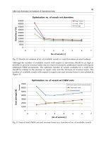
For completeness sake, Fig. 8 shows the wind resource maps for the JARBO station referred
to wind speed and power density at 20 metres high. The wind speed obtained in this area
ranges from 1.70 to 2.38 m/s and the wind power variation goes from 7 to 18 W/m
2
, which
can hardly make a case for installing a wind turbine.



(a) ( b)
Fig. 8. Wind resource maps for (a) wind speed and (b) power density at the JARBO station
produced with the use of the WAsP package

Wind Farm – Technical Regulations, Potential Estimation and Siting Assessment

108
5.3 Case study: rural areas
In this case, the surveyed data stems from measurements taken at a monitoring station
located in the UAA-UAZ rural and farming area (Medina, 2006; IIE, 2008). These readings
were taken at three different altitudes, namely 3, 20 and 40 metres above ground level.
Three friction coefficients were obtained from this data while resorting to equation (3) at 3
and 20 metres (
α
1
), at 3 and 40 metres (α
2
) and, finally, at 20 and 40 metres (α
3
). With these
friction coefficients the relevant roughness coefficients and their average values were
calculated using equation. (6). Thereafter we calculated the annual average values for the
friction and roughness coefficient at 0.240 and 0.181 m respectively. The average speeds of
every month and the annual average were calculated with the use of both friction and
roughness coefficients. We then undertook a comparison between calculated and measured
data at 20 and 40 metres high and we identified some variations. Tables 6 and 7 show the
sets of calculated and measured data as well as highlighting the differences between them;
in some cases in excess of 8%, as shown in the average speed columns calculated for 40 m
(
V
3
in August, column 4 from Table 6 and column 5 from Table 7) with both friction and
roughness coefficients at the

H
1
and H
3
altitudes.

Month
V
1
(1)
V
2
(2)
V
3

(3)
α
1

(4)
α
2

(5)
α
3

(6)
Zo

(7)
Zo
(8)
Zo
(9)
August-2005 2.02 3.92 4.25 0.350 0.287 0.117 0.400 0.288 0.005
September 2005 2.53 4.55 5.03 0.309 0.265 0.145 0.279 0.218 0.028
October 2005 2.22 3.99 4.47 0.309 0.270 0.164 0.278 0.233 0.063
November 2005 2.04 3.78 4.34 0.325 0.292 0.199 0.325 0.302 0.186
December 2005 1.75 3.66 4.14 0.387 0.331 0.178 0.521 0.445 0.101
January 2006 2.20 4.18 4.63 0.337 0.286 0.148 0.360 0.284 0.032
February 2006 2.23 4.10 4.62 0.321 0.281 0.172 0.312 0.268 0.085
March 2006 2.92 4.83 5.47 0.265 0.242 0.180 0.165 0.155 0.107
April 2006 2.71 4.39 4.9 0.252 0.227 0.159 0.137 0.119 0.051
May 2006 2.63 4.34 4.85 0.264 0.236 0.160 0.162 0.139 0.055
June 2006 3.06 4.77 5.21 0.234 0.205 0.127 0.100 0.075 0.011
July 2006 2.84 4.40 4.91 0.231 0.211 0.158 0.095 0.086 0.051
Annual average 2.43 4.24 4.73 0.299 0.261 0.159 0.261 0.218 0.065
Notes:
(1) Speed averages, at
H1 = 3 m, in m/s
(2) Speed averages, at
H2 = 20 m, in m/s
(3) Speed averages, at
H3 = 40 m, in m/s
(4) Friction coefficient, monthly average using measurements at
H1, H2, V
1
, V

2
and Eq. (5)
(5) Friction coefficient, monthly average using measurements
at H1, H3, V
1
, V
3
and Eq. (5)
(6) Friction coefficient, monthly average using measurements
at H2, H3, V
2
, V
3
and Eq. (5)
(7) roughness coefficient, monthly average using measurements
at H1, H2, V
1
, V
2
and Eq. (6), in m.
(8) Roughness coefficient, monthly average using measurements
at H1, H3, V
1
, V
3
and Eq. (6), in m.
(9) Roughness coefficient, monthly average using measurements
at H2, H3, V
2
, V

3
and Eq. (6) in m.
Table 6. Data and results for average friction and roughness coefficients in rural areas