Chaotic Systems Part 3 docx
Bạn đang xem bản rút gọn của tài liệu. Xem và tải ngay bản đầy đủ của tài liệu tại đây (4.54 MB, 25 trang )
3
Relationship between the Predictability Limit
and Initial Error in Chaotic Systems
Jianping Li and Ruiqiang Ding
State Key Laboratory of Numerical Modeling for Atmospheric Sciences and
Geophysical Fluid Dynamics, Institute of Atmospheric Physics,
Chinese Academy of Sciences, Beijing 100029
China
1. Introduction
Since the pioneer work of Lorenz on predictability problems [1–2], many studies have
examined the relationships between predictability and initial error in chaotic systems [3–7];
however, these previous studies focused on multi-scale complex systems such as the
atmosphere and oceans [4–6]. Because large uncertainties exist regarding the dynamic
equations and observational data related to such complex systems, there also exists
uncertainty in any conclusions drawn regarding the relationship between the predictability
of such systems and initial error. In addition, multi-scale complex systems such as the
atmosphere are thought to have an intrinsic upper limit of predictability due to interactions
among different scales [2, 4–6]. The predictability time of multi-scale complex systems,
regardless of the errors in initial conditions, cannot exceed their intrinsic limit of
predictability.
For relatively simple chaotic systems with a single characteristic timescale driven by a small
number of variables (e.g., the logistic map [7] and the Lorenz63 model [1]), their predictability
limits continuously depend on the initial errors: the smaller the initial error, the greater the
predictability limit. If the initial perturbation is of size
0
δ
and if the accepted error tolerance,
Δ , remains small, then the largest Lyapunov exponent
1
Λ
gives a rough estimate of the
predictability time:
10
1
~ln()
p
T
Λ
δ
Δ
. However, reliance on the largest Lyapunov exponent
commonly proves to be a considerable oversimplification [8]. This generally occurs because
the largest Lyapunov exponent
1
Λ
, which we term the largest global Lyapunov exponent, is
defined as the long-term average growth rate of a very small initial error. It is commonly the
case that we are not primarily concerned with averages, and, even if we are, we may be
interested in short-term behavior. Consequently, various local or finite-time Lyapunov
exponents have been proposed, which measure the short-term growth rate of initial small
perturbations [9–12]. However, the existing local or finite-time Lyapunov exponents, which
are the same as the global Lyapunov exponent, are established based on the assumption that
the initial perturbations are sufficiently small that their evolution can be approximately
governed by the tangent linear model (TLM) of the nonlinear model, which essentially belongs
to linear error dynamics. Clearly, as long as an uncertainty remains infinitesimal in the
Chaotic Systems
40
framework of linear error dynamics, it cannot pose a limit to predictability. To determine the
limit of predictability, any proposed ‘local Lyapunov exponent’ must be defined with respect
to the nonlinear behavior of nonlinear dynamical systems [13–14].
Recently, the nonlinear local Lyapunov exponent (NLLE) [15–17], which is a nonlinear
generalization to the existing local Lyapunov exponents, was introduced to study the
predictability of chaotic systems. NLLE measures the averaged growth rate of initial errors of
nonlinear dynamical models without linearizing the governing equations. Using NLLE and its
derivatives, the limit of dynamical predictability in large classes of chaotic systems can be
efficiently and quantitatively determined. NLLE shows superior performance, compared with
local or finite-time Lyapunov exponents based on linear error dynamics, in determining
quantitatively the predictability limit of chaotic system. In the present study, we explore the
relationship between the predictability limit and initial error in simple chaotic systems based
on the NLLE approach, taking the logistic map and Lorenz63 model as examples.
2. Nonlinear local Lyapunov exponent (NLLE)
For an n-dimensional nonlinear dynamical system, its nonlinear perturbation equations are
given by:
() ()() ( )
d
t
dt
= ttδ Jx δ
+ () ()(,)ttGx δ , (1)
where
T
1
()=(
2
(), (), , ())
n
txt xt""txx is the reference solution, T is the transpose,
() ()()ttJx δ
are the tangent linear terms, and
() ()(,)ttGx δ
are the high-order nonlinear terms of the
perturbation
T
12
() ( (), (), , ())
n
ttt t
δδ δ
= ""δ . Most previous studies have assumed that the
initial perturbations are sufficiently small that their evolution could be approximately
governed by linear equations [9–12]. However, linear error evolution is characterized by
continuous exponential growth, which is not applicable to the description of a process that
evolves from initially exponential growth to finally reaching saturation for sufficiently small
errors (see Fig. 1). This linear approximation is also not applicable to situations in which the
initial errors are not very small. Therefore, the nonlinear behaviors of error growth should
be considered to determine the limit of predictability. Without linear approximation, the
solutions of Eq. (1) can be obtained by numerical integration along the reference solution
()tx
from
0
=tt
to
0
τ
+
t
:
0
()
000
()(,(),)()ttt
ττ
+= tδηx δδ, (2)
where
0
()
0
(,(),)t
τ
tη x δ
is the nonlinear propagator. NLLE is then defined as
0
()
0
0
0
()
1
(,(),)ln
()
t
t
t
τ
λτ
τ
+
=
t
δ
x δ
δ
, (3)
where
0
()
0
(,(),)t
λ
τ
tx δ depends in general on the initial state
0
()tx in phase space, the initial
error
0
()tδ , and time
τ
. This differs from the existing local or finite-time Lyapunov
exponents, which are defined based on linear error dynamics [9–12]. In the case of double
limits of
0
() 0t →δ and
τ
→∞, NLLE converges to the largest global Lyapunov exponent
1
Λ
. The ensemble mean NLLE over the global attractor of the dynamical system is given by
Relationship between the Predictability Limit and Initial Error in Chaotic Systems
41
000
λ
(( ),) λ(( ),( ),)tttd
ττ
Ω
=
∫
δ x δ x
00
λ
(( ),( ),)
N
tt
τ
= x δ , ( N →∞) (4)
where Ω represents the domain of the global attractor of the system, and
N
denotes the
ensemble average of samples of sufficiently large size N (N →∞). The mean relative
growth of initial error (RGIE) can be obtained by
00
() ()(,)exp((,))E
τ
λττ
=ttδδ. (5)
Using the theorem from Ding and Li [16], then we obtain
0
(( ),)
P
Et c
τ
⎯
⎯→δ ( N →∞), (6)
where
P
⎯
⎯→ denotes the convergence in probability and c is a constant that depends on
the converged probability distribution of error growth
P . This is termed the saturation
property of RGIE for chaotic systems. The constant
c
can be considered as the theoretical
saturation level of
0
(( ),)Et
τ
δ
. Once the error growth reaches the saturation level, almost all
information on initial states is lost and the prediction becomes meaningless. Using the
theoretical saturation level, the limit of dynamical predictability can be determined
quantitatively [15–16]. In addition, for
00
1
(( ),) ln (( ),)tEt
t
λ
ττ
⎡
⎤
=
⎣
⎦
δδ, based on the above
analysis, we have
0
1
(( ),) ln
P
tc
λτ
τ
⎯⎯→×δ
as
τ
→∞; (7)
therefore,
0
(( ),)t
λ
τ
δ asymptotically decreases like O( 1
τ
) as
τ
→∞. The magnitude of the
initial error
δ
0
is defined as the norm of the vector error
0
()tδ in phase space at the initial
time
0
t ; i.e.,
00
()t
δ
= δ . The results show that the limit of dynamical predictability depends
mainly on the magnitude of the initial error
0
()tδ
and rather than on its direction, because
the error direction in the phase space becomes rapidly aligned toward the most unstable
direction (Fig. 2).
3. Experimental predictability results
The first example is the logistic map [7],
1
(1 )
nnn
y
ay y
+
=
− , 0 4a
≤
≤ , (8)
Here, we choose the parameter value of a
=
4.0, for which the logistic map is chaotic on the
set (0,1) [18–19]. Figure 3 shows the dependence of the mean NLLE and the mean RGIE on
the magnitude of the initial error. The mean NLLE is essentially constant in a plateau region
that widens as decreasing initial error
δ
0
(Fig. 3a). For a sufficiently long time, however, all
the curves are asymptotic to zero. This finding reveals that for a very small initial error,
Chaotic Systems
42
error growth is initially exponential, with a growth rate consistent with the largest global
Lyapunov exponent, indicating that linear error dynamics are applicable during this phase.
Subsequently, the error growth enters a nonlinear phase with a steadily decreasing growth
rate, finally reaching a saturation value.
Figure 3b shows that the time at which the error growth reaches saturation also lengthens as
δ
0
is reduced. Regardless of the magnitude of the initial error
δ
0
, all the errors ultimately
reach saturation. To estimate the predictability time of a chaotic system, the predictability
limit is defined as the time at which the error reaches 99% of its saturation level. The limit of
dynamic predictability is found to decrease approximately linearly as increasing logarithm
of initial error (Fig. 4). For a specific initial error, the limit of dynamic predictability is longer
than the time for which the tangent linear approximation holds, which is defined as the time
over which the mean NLLE remains constant. The difference between the predictability
limit and the time over which the tangent linear approximation holds, remains largely
constant as increasing logarithm of initial error, suggesting that the time over which the
nonlinear phase of error growth lasts may be constant for initial errors of various
magnitudes.
The second example is the Lorenz63 model [1],
XXY
YrXYXZ
ZXYbZ
σσ
⎧
=− +
⎪
⎪
=−−
⎨
⎪
=−
⎪
⎩
, (9)
where σ =10, r =28, and b =8/3, for which the well-known “butterfly” attractor exists.
Figure 5 shows the mean NLLE and mean RGIE with initial errors of various magnitudes as
a function of time
τ
. For all initial errors, the mean NLLE is initially unstable, then remains
constant and finally decreases rapidly, approaching zero as increasing
τ
(Fig. 5a). For a very
small initial error, it does not take long for error growth to become exponential, with a
growth rate consistent with the largest global Lyapunov exponent, indicating that linear
error dynamics are applicable during this phase. Subsequently, error growth enters a
nonlinear phase with a steadily decreasing growth rate, finally reaching a saturation value
(Fig. 5b). For initial errors of various magnitudes, the predictability limit of the Lorenz63
model is defined as the time at which the error reaches 99% of its saturation level, similar to
the case for the logistic map.
Figure 6 shows the predictability limit and the time over which the tangent linear
approximation holds as a function of the magnitude initial error. The predictability limit of
the Lorenz63 model decreases approximately linearly as increasing logarithm of initial error,
similar to the logistic map. For the Lorenz63 model, the difference between the predictability
limit and the time over which the tangent linear approximation holds, remains largely
constant as increasing logarithm of initial error.
4. Theoretical predictability analysis
As shown above, there exists a linear relationship between the predictability limit and the
logarithm of initial error, for both the logistic map and Lorenz63 model. To understand the
reason for this linear relationship, it is necessary to further investigate the relationship
between the predictability limit and the logarithm of initial error using the theoretical
Relationship between the Predictability Limit and Initial Error in Chaotic Systems
43
analysis, to determine if a general law exists between the predictability limit and the
logarithm of initial error for chaotic systems.
For relatively simple chaotic systems such as the logistic map and Lorenz63 model, the
predictability limit
p
T
is assumed to consist of the following two parts:
p
LN
TTT
=
+ , (10)
where
L
T is the time over which the tangent linear approximation holds, and
N
T is the time
over which the nonlinear phase of error growth occurs. When the mean error reaches a
critical value
c
δ
, which is thought to be almost constant for a chaotic system under the
condition of the given parameters, the tangent linear approximation is no longer valid and
the error growth enters the nonlinear phase. Under the condition of the given parameters,
the saturation value of error
*
E is constant, which is not dependent on the initial error.
Consequently, the time
N
T taken for the error growth from
c
δ
to
*
E can be considered as
almost constant, not relying on the initial error. This assumption is confirmed by the
experimental results shown in Figs. 3 and 5, which indicate that the interval between the
predictability limit and the time over which the tangent linear approximation holds, remains
almost constant as increasing logarithm of initial error. Then,
N
T can be written as a
constant:
1N
TC
=
. (11)
For
L
T , the time over which the tangent linear approximation holds, we get
1
()
cL
T
δ
δΛ
0
=
exp , (12)
where
δ
0
is the initial error and
1
Λ
is the largest global Lyapunov exponent. From Eq. (12),
we have
1
1
ln
c
L
T
δ
Λ
δ
0
⎛⎞
=
⎜⎟
⎝⎠
. (13)
From Eqs. (10), (11), and (13), we obtain
[]
1
1
1
ln ln
pc
TC
δ
δ
Λ
0
=+ − . (14)
Under the condition of the given parameters,
1
Λ
of the chaotic system is fixed, as is
1
1
ln
c
δ
Λ
. Then, we have
2
1
1
ln
c
C
δ
Λ
= (where
2
C is a constant). Therefore,
p
T
can be written
as
1
1
ln
p
TC
δ
Λ
0
=− , (15)
where
12
CC C=+. Eq. (15) can be changed to
Chaotic Systems
44
o
o
10
110
lg
1
lg
p
TC
e
δ
Λ
0
=− . (16)
If the largest global Lyapunov exponent
1
Λ
and the constant C are known in advance, the
predictability limit can be obtained for initial errors of any magnitude, according to Eq. (16).
The constant
C can be calculated from Eq. (16) if the predictability limit corresponding to a
fixed initial error has been obtained in advance through the NLLE approach.
5. Experimental verification of theoretical results
Using the method proposed by Wolf et al. [20], the largest global Lyapunov exponent
1
Λ
of the logistic map is 0.693 when 4.0
a
=
. From Eq. (16), we have the formula that
describes the relationship between the predictability limit and the initial error of the
logistic map:
o
10
3.32l g
p
TC
δ
0
=
− . (17)
For
6
10
δ
−
0
= , the predictability limit of the logistic map is 18
p
T
=
, as obtained using the
NLLE approach. Then, we have 1.92
C
=
− in Eq. (17). Therefore, the predictability limit for
various initial errors can be obtained from Eq. (17). The predictability limits obtained in this
way are in good agreement with those obtained using the NLLE approach (Fig. 7). This
finding indicates that the assumptions presented in Section 3 are indeed reasonable.
Therefore, it is appropriate to determine the predictability limit of the logistic map by
extrapolating Eq. (17) to various initial errors.
The largest global Lyapunov exponent
1
Λ
of the Lorenz63 model is obtained to be 0.906
when
σ
=10, r =28, b =8/3. From Eq. (16), we have the formula that describes the
relationship between the predictability limit and the initial error of the Lorenz63 model:
o
10
2.54l g
p
TC
δ
0
=
− . (18)
For
6
10
δ
−
0
= , the predictability limit of the Lorenz63 model is 22.19
p
T
=
, as obtained using
the NLLE approach. Then, we have 6.95
C
=
in Eq. (17). Therefore, the predictability limits
for various initial errors can be obtained by extrapolating the Eq. (17) to various initial
errors. The resulting limits are in good agreement with those obtained using the NLLE
approach (Fig. 8). The linear relationship between the predictability limit and the logarithm
of initial error is further verified by the Lorenz63 model, and the relationship may be
applicable to other simple chaotic systems.
6. Summary
Previous studies that examine the relationship between predictability and initial error in
chaotic systems with a single characteristic timescale were based mainly on linear error
dynamics, which were established based on the assumption that the initial perturbations are
sufficiently small that their evolution could be approximately governed by the TLM of the
nonlinear model. However, linear error dynamics involves large limitations, which is not
applicable to determine the predictability limit of chaotic systems.
Relationship between the Predictability Limit and Initial Error in Chaotic Systems
45
Taking the logistic map and Lorenz63 model as examples, we investigated the relationship
between the predictability limit and initial error in chaotic systems, using the NLLE
approach, which involves nonlinear error growth dynamics. There exists a linear
relationship between the predictability limit and the logarithm of initial error. A theoretical
analysis performed under the nonlinear error growth dynamics revealed that the growth of
mean error enters a nonlinear phase after it reaches a certain critical magnitude, finally
reaching saturation. For a given chaotic system, if the control parameters of the system are
given, then the saturation value of error growth is fixed. The time taken for error growth
from the nonlinear phase to saturation is also almost constant for various initial errors. The
predictability limit is only dependent on the phase of linear error growth. Consequently,
there exists a linear relationship between the predictability limit and the logarithm of initial
error. The linear coefficient is related to the largest global Lyapunov exponent: the greater
the latter, the more rapidly the predictability limit decreases as increasing logarithm of
initial error. If the largest global Lyapunov exponent and the predictability limit
corresponding to a fixed initial error are known in advance, the predictability limit can be
extrapolated to various initial errors based on the linear relationship between the
predictability limit and the logarithm of initial error.
It should be noted that the linear relationship between the predictability limit and the
logarithm of initial error holds only in the case of relatively small initial errors. If the initial
errors are large, the growth of the mean error would directly enter into the nonlinear phase,
meaning that the linear relationship would fail to describe the relationship between the
predictability limit and the logarithm of initial error. A more complex relationship may exist
between the predictability limit and initial errors, which is an important subject left for
future research.
7. Acknowledgment
This research was funded by an NSFC Project (40805022) and the 973 program
(2010CB950400).
Fig. 1. Linear (dashed line) and nonlinear (solid line) average growth of errors in the Lorenz
system as a function of time. The initial magnitude of errors is 10
–5
.
Chaotic Systems
46
Fig. 2. Mean NLLE
0
(( ),)t
λ
τ
δ (a) and the logarithm of the corresponding mean RGIE
0
(( ),)Et
τ
δ (b) in the Lorenz63 model as a function of time
τ
. In (a) and (b), the dashed and
solid lines correspond to the initial errors
0
()tδ = (10
–6
, 0, 0) and
0
()tδ = (0, 0, 10
–6
),
respectively.
Fig. 3. Mean NLLE
0
(( ), )tn
λ
δ (a) and the logarithm of the corresponding mean RGIE
0
(( ), )Etnδ (b) in the logistic map as a function of time step
n
and
0
δ
of various
magnitudes. From above to below, the curves correspond to
0
δ
=10
–12
, 10
–11
, 10
–10
, 10
–9
, 10
–8
,
10
–7
, 10
–6
, 10
–5
, 10
–4
, and 10
–3
, respectively. In (a), the dashed line indicates the largest global
Lyapunov exponent.
Relationship between the Predictability Limit and Initial Error in Chaotic Systems
47
Fig. 4. Predictability limit
P
T
and the time
L
T
over which the tangent linear approximation
holds in the logistic map as a function of
0
δ
of various magnitudes.
Fig. 5. Same as Fig. 3, but for the Lorenz63 model.
Chaotic Systems
48
Fig. 6. Same as Fig. 4, but for the Lorenz63 model.
Fig. 7. Predictability limits obtained from Eq. (17) (open circles) and those obtained using the
NLLE approach (closed triangles) in the logistic map as a function of
0
δ
of various
magnitudes.
Relationship between the Predictability Limit and Initial Error in Chaotic Systems
49
Fig. 8. Same as Fig. 7, but for the Lorenz63 model.
8. References
[1] E. N. Lorenz, J. Atmos. Sci. 20 (1963) 130.
[2] E. N. Lorenz, J. Atmos. Sci. 26 (1969) 636.
[3] J. P. Eckmann, D. Ruelle, Rev. Mod. Phys. 57 (1985) 617.
[4] Z. Toth, Mon. Wea. Rev. 119 (1991) 65.
[5] W. Y. Chen, Mon. Wea. Rev. 117 (1989) 1227.
[6] V. Krishnamurthy, J. Atmos. Sci. 50 (1993) 2215.
[7] R. M. May, Nature 261 (1976) 459.
[8] E. N., Lorenz, in Proceedings of a Seminar Held at ECMWF on Predictability
(I),
European Centre for Medium-Range Weather Forecasts, Reading, UK, 1996, p. 1.
[9] J. M. Nese, Physica D 35 (1989) 237.
[10] E. Kazantsev, Appl. Math. Comp. 104 (1999) 217.
[11] C. Ziemann, L. A. Smith, J. Kurths, Phys. Lett. A 4 (2000) 237.
[12] S. Yoden, M. Nomura, J . Atmos. Sci . 50 (1993) 1531.
[13] J. F. Lacarra, O. Talagrand, Tellus 40A (1988) 81.
[14] M. Mu, W. S. Duan, B. Wang, Nonlinear Process. Geophys. 10 (2003) 493.
[15] J. P. Li, R. Q. Ding, B. H. Chen, in Review and prospect on the predictability study of the
atmosphere,
Review and Prospects of the Developments of Atmosphere Sciences in Early
21st Century
, China Meteorology Press, 96.
[16] R. Q. Ding, J. P. Li,
Phys. Lett. A 364 (2007) 396.
[17] R. Q. Ding, J. P. Li, K. J. Ha,
Chin. Phys. Lett. 25 (2008) 1919.
[18] C. Rose, M. D. Smith, Mathematical Statistics with Mathematica, Springer-Verlag, New
York, 2002.
Chaotic Systems
50
[19] J. Guckenheimer, P. J. Holmes, Nonlinear Oscillations, Dynamical Systems, and
Bifurcations of Vector Fields, Springer-Verlag, New York, 1983.
[20] A. Wolf, J. B. Swift, H. L. Swinney, J. A. Vastano, Physica D 16 (1985) 285.
0
Microscopic Theory of Transport Phenomenon in
Hamiltonian Chaotic Systems
Shiwei Yan
College of Nuclear Science and Technology, Beijing Normal University
China
1. Introduction
It has been one of the important fields of contemporary science to explore the microscopic
origin of the damping phenomenon of collective motion in the finite many-body system.
The evolution of the early universe, that of the chemical reaction, many active processes
in biological system, the fission and fusion processes in nuclear system, the quantum
correspondent of the classically chaotic system and the measurement theory are typical
examples among others(1–14). Although these processes have been successfully described
by the phenomenological transport equation, there still remain some basic problems, such
as, how to derive the macro-level transport equation describing the macroscopic irreversible
motion from the micro-level reversible dynamics from the fundamental level dynamics; how
the statistical state is realized in the irrelevant subsystem and why the irreversible macro-level
process is generated as a result of the reversible micro-level dynamics.
The study on this subject has been one of the most fundamental and challenging fields in
the various fields of contemporary science. Intensive studies have been carried out (15–29),
however, an acceptance microscopic understanding is still far from realization and there still
remain a lot of studies(30–33).
1.1 From reversible to irreversible: Foundation of statistical physics
Before discussing the microscopic origin of irreversibility phenomenon, one should be aware
of an informal indication of the problem in explaining the meaning of the foundation
of statistical physics, which can be seen in the presence of two types of processes: (1)
time-irreversible macroscopic (relevant or collective) process which obey the thermodynamics,
or kinetic, laws; and (2) time-reversible microscopic (irrelevant or intrinsic)processwhich
obey, say, the Newton and Maxwell equations of motion. The great difference between
both descriptions of the processes in nature, is not clearly understood and an acceptance
explanation on the origin of irreversibilityis still lack(34). The formal definition of the problem
is to derive a macroscopic equation which describes an irreversible evolution which begins
with a reversible Hamiltonian equation.
Before the recognition of the importance of chaos, the attempts to unite, in a formal way,
the statistical and dynamical description of a system, usually starts with dividing the total
system into the relevant and irrelevant degrees of freedom by hand and assuming the
irrelevant system placed in a state of micro-canonical equilibrium (thermodynamical) state
4
(Ref. Boltzmann’s pioneer proposal(35) and the textbooks as (36)). This is the Boltzmann
principle
S
= k ln A(E).(1)
where
A(E) is the area of the phase space explored by the system in a micro-canonical state,
k the Boltzmann constant and S the entropy. However, such the derivations are essentially
based on the assumption of an infinitely large number of degrees of freedom and the existence
of two different time scales τ
r
τ
i
,whereτ
r
is the time scale of relevant degrees of freedom
and τ
i
is that of irrelevant ones. Under such assumption, the irreversibility or the equilibrium
condition is supplemented for the dynamical equations, and the resultant distribution has the
form
P
() ∼ e
−β
β ≡ 1/kT (2)
where is the energy of the irrelevant degrees of freedom and T the temperature of the system.
Distribution (2) is called the equilibrium Boltzmann distribution which corresponds to the
thermodynamical state and thus only can be adopted to describe the equilibrium process rather
than nonequilibrium states. It also should be mentioned that Poincar
´
e recurrence theorem says
that for a finite and area-preserving motion, any trajectory should return to an arbitrarily
taken domain Σ in a finite time and should do so repeatedly for an infinite number of time.
However, Boltzmann had rightly argue that for a large number of particles, this recurrence
time would be astronomically long. This assumption only can be justified for a system with
infinite number of degrees of freedom. When one want to study the origin of irreversibility
of a finite system where dynamical chaos occurs, this assumption of infinite occurrence time
will cause some serious problems.
Many attempts have been successfully achieved in different ways and with some
supplementary conditions on microscopic Hamiltonian equations, such as the random phase
approximation (mixing)(37; 38), Gaussian orthogonal ensemble (GOE), or other equivalent
conditions played the role of statistical element(15–20; 25–29; 39). The ergodic and irreversible
property is assumed for the irrelevant system with infinite number of degree of freedom.
Temperature, so as thermodynamics, is introduced by hand through the supplementary
conditions. From dynamical point of view, such the derivation is unsatisfactory since the
strong condition like randomness of some variables or statistical ansatz should be introduced
by hand. Following the recognition of the importance of chaos, it has been supposed that there
is an intimate relation between the realization of irreversibility and the order-to-chaos transition within
the microscopic Hamilton dynamics. When one derives the macroscopic irreversibility from
the fundamental Hamiltonian equations, the stochastic processes can be obtained for some
specific parameters and initial conditions. However even in this case, such the supplementary
assumptions still remain to be justified. The main problems are: whether or not one may
substantiate statistical state in the way dynamical chaos is structured in real Hamiltonian
system, whether or not there are some difficulties of using the properties of dynamical chaos as
a source of randomness, whether one can derive a random process from the dynamical chaotic
motion and whether or in what conditions, the derived stochastic process may correspond
to the above-mentioned random assumptions. It is well known that Poincar
´
erecurrence
time is finite for finite Hamiltonian systems and its phase space has fractal (or multi-fractal)
structure, where the ergodicity of motion is not generally satisfied. Therefore, specially in
the finite system, it is not a trivial discussion whether or not the irrelevant subsystem can be
effectively replaced by a statistical object as a heat bath, even when it shows chaotic behavior
52
Chaotic Systems
and its Lyapunov exponent has a positive value everywhere in the phase space. It is also an
interesting question to explore the relation between the dynamical definition of the statistical
state, if it exists, and the static definition of it.
1.2 From infinite to finite system
It should say that there is substantial difficulty, or it is almost impossible in some extent, for
us to derive the macroscopic irreversibility from the fundamental Hamiltonian equations for
an infinite system because which has an infinite (or extremely large) number of degrees of
freedom. This fact is generally accepted as the reason for the introduction of the statistical
assumptions. On another hand, when one derive macroscopic equations by averaging over
microscopic random variables resulted in a reduced description of an innite system, the
detailed structure of micro phase space will lose its importance. In this sense, for an innite
system, such the statistical approach seems to be reasonable and will not cause any serious
problems.
However, in such systems as atoms, nuclei and biomolecules whose environment is not
infinite, where assumption of a large number of degrees of freedom is not justified, and
in a case when one intends to derive the macroscopic irreversibility and phenomenological
transport equation from the fundamental level dynamics, it is not obvious whether or not one
may introduce the statistical assumptions for the irrelevant degrees of freedom. The decisive
problem in the finite system is how to justify an introduction of some statistical state or some
statistical concept like the temperature or the heat bath, which is one of the basic ingredient to
derive an irreversible process to the Hamilton system.
With regards to the damping phenomena observed in the giant resonance on top of the
highly excited states in the nuclear system, its microscopic description has been mainly
based on the temperature dependent mean-field theory(40–45). However, an introduction
of the temperature in the finite-isolated nuclei is by no means obvious, when one explicitly
introduce many single-particle excitation modes on top of the temperature-dependent shell
model. Could one introduce a chaotic (complex) excitation mode on top of the chaotic (heat
bath characterized by the temperature) system? When one considers the 2p-2h (two-particle
two-hole) state as a door way state to be coupled with the 1p-1h collective excitation mode,
a naive classical model Hamilton would be something like a β Fermi-Pasta-Ulam (FPU)
system(46–49) where no heat bath is assumed, rather than the temperature-dependent shell
model where the Matsubara Green function is used.
The recent development in the classical theory of nonlinear Hamiltonian system (22; 34; 50–
53) has shown that there appears an exceedingly rich structure in the phase space, which is
usually considered to prevent a fully developed chaos. The existence of fractal structure is a
remarkable property of Hamilton chaos and a typical feature of the phase space in real system.
Due to the fractal structure of the phase space, the motion of Hamilton system of general type
is not ergodic, specially for a finite Hamiltonian system. In this case, the questions then arise:
what kind random process corresponds to the dynamical chaotic motion? whether or not
the system dynamically reaches some statistical object? The microscopic derivation of the
non-equilibrium statistical physics in relation with the exceedingly rich structure of the phase
space as well as with the order-to-chaos transition might be explored within the microscopic
Hamilton dynamics. This subject will be further discussed in Sec. 4.1.2.
Another important issue related to this study is how to divide the total system into the relevant
and irrelevant degrees of freedom. However, in many approaches(24; 26; 27), one usually
starts with dividing the total system into the relevant and irrelevant degrees of freedom
53
Microscopic Theory of Transport Phenomenon in Hamiltonian Chaotic Systems
by hand. In the system where a total number of degrees of freedom can be approximately
treated as an infinite, there does not arise any serious problem how to introduce the relevant
degrees of freedom. In the finite system as nuclei where a number of the degrees of freedom
is not large enough, and a time scale of the relevant motion and that of the irrelevant one
is typically less than one order of magnitude difference, there arises an important problem
how to distinguish the relevant ones from the rest in a way consistent with the underlying
microscopic dynamics for aiming to properly characterize the collective motion. Here it worth
to mention another important issue is related with an applicability of the linear response theory
(LRT)(54–59), because a validity of the linear approximation for the macro-level dynamics
does not necessarily justify that for the micro-level dynamics. Furthermore, there arises a
basic question whether or not one may divide the total system into the relevant and irrelevant
subsystems by leaving the linear coupling between them(30; 50; 60–62). At the best of our
knowledge, it seems that there is no compelling physical reason to choose the linear coupling
interaction between the relevant and irrelevant subsystems.
Summarily speaking, in exploring the microscopic dynamics in nite Hamiltonian system,says,
answering the basic questions as listed in the beginning of this section, there are two main
subjects. One is how to divide the total system into the relevant and irrelevant ones and another is how
to derive the macroscopic statistical properties from microscopic dynamics.
1.3 The nonlinear theory of the classical Hamiltonian system
From above discussion, one can conclude that the theory of chaotic dynamics should play a
decisive role in understanding the origin of microscopic irreversibility within the microscopic
Hamilton dynamics. It is imperative to remember the recent development in the classical
theory of nonlinear Hamilton system(34; 51–53).
The chaos phenomenon is often used to describe the motions of the system’s trajectories
which are sensitive to the slightest changes of the initial condition. The motion known as
chaotic occupies a certain area (called stochastic sea) in the phase space. In idea chaos,
the stochastic sea is occupied in uniform manner. This is, however, not the case in real
systems. The phase space has exceedingly rich structure where the chaotic and regular
motions co-exist and there are many islands which a chaotic trajectory can not penetrate
(as stated in KAM Theorem). Many important properties of chaotic dynamics, such as the
order-to-chaos transition dynamics, are determined by the properties of the motion near the
boundary of islands.
Thanks to H. Poincaré and his successors, we know how important it is to understand why
there appears an exceedingly rich structure in the phase space and how the order-to-chaos
transition occurs, rather than to understand individual trajectory under a specific initial
condition. A set of closed orbits having the same property (characterized by a set of local
constants of motion) forms a torus structure around a certain stable fixed point in the phase
space, and is separated from the other types of closed orbits (characterized by another set of
local constants of motion) through separatrices. Depending on the strength of the nonlinear
interaction or on the energy of the system, there appear many kinds of new periodic orbits
characterized by respective local constants of motion along the known periodic orbits, which
are called bifurcation phenomena.
When different separatrices start to overlap in a small region of the phase space, there appears
a local chaotic sea. In this overlap region where two kinds of periodic orbits characterized
by different sets of constants of motion start to coexist, it might become difficult to realize
a well-developed closed orbit characterized by a single set of local constants of motion any
54
Chaotic Systems
-1
-0.5
0
0.5
1
-1 -0.5 0 0.5 1
P1
Q1
Fig. 1. Poincaré section map of SU(3) Hamiltonian on (q
1
, p
1
)planeforacasewithE = 40
and V
i
= −0.01
more. This overlap criterion on an appearance of the chaotic sea has been considered to be a
microscopic origin of the order-to-chaos transition dynamics.
A classical example of the order-to-chaos transition for the SU(3) classical Hamiltonian system
(66) is shown in Figs. 1 to 4 for the cases with V
i
=-0.01, -0.03, -0.045 and -0.07, respectively. In
the cases with V
i
=-0.01 and -0.03, i.e., the smaller interaction strength or weaker nonlinearity,
the whole phase space is covered by the regular motions, forming many islands structure.
When the nonlinearity of interaction goes to stronger, there appears chaotic sea in a region
where the crossing point of the separatrics (Fig. 3), i.e., the unstable fixed point is expected in
Fig. 2. Moreover, there appear many secondary islands around the primary island structure,
which has already existed in Fig. 2. A chaotic trajectory can not penetrate the island and a
regular trajectory from an island is not be able to escape from it. Around some secondary
island, one may find some tertiary island structure, and so forth, as shown in Fig. 5. This
repeated complex structure is called fractal phenomena. The fractal structure of phase space
is a remarkable property of Hamiltonian chaos and a typical feature of the phase space in
real systems. For a classical Hamiltonian system, the distribution of the Poincar
´
erecurrence
is time- and space-fractal, which plays a crucial role in an understanding of the general
properties of chaotic dynamics and the foundation of statistical physics.
The general theory of the nonlinear dynamics has been developed for aiming to understand
these complex structure by studying why there appear many stable and unstable fixed points,
and how to get an information on their constants of motion. And also the theory of nonlinear
chaotic dynamics plays an important role in understanding the foundation of statistical
physics.
55
Microscopic Theory of Transport Phenomenon in Hamiltonian Chaotic Systems
-1
-0.5
0
0.5
1
-1 -0.5 0 0.5 1
P1
Q1
Fig. 2. Poincaré section map of SU(3) Hamiltonian on (q
1
, p
1
)planeforacasewithE = 40
and V
i
= −0.03
1.4 The self-consistent collective coordinate (SCC) method & the optimum coordinate
system
As discussed in Sect. 1.2, for finite system, an important problem is to explore how to divide
the total system into the relevant and irrelevant degrees of freedom in a way consistent
with the underlying microscopic dynamics for aiming to properly characterize the collective
motion. In a case of the Hamiltonian system, a division may be performed by applying
the self-consistent collective coordinate (SCC) method(60). In the following, for the sake of
self-containedness, the SCC method is briefly reformulated within the classical Hamiltonian
system. The detailed description can be found in Ref. (60) and a review article (50).
The SCC method was proposed within the usual symplectic manifold, which intends to
define the maximally-decoupled coordinate system where the minimum number of coordinates is
required in describing the trajectory under discussion. In such a finite system as the nucleus,
it is not obvious how to introduce the relevant (collective or distinguished) coordinates which
are used in describing macroscopic properties of the system. This problem is also very
important to explore why and how the statistical aspect could appear in the finite nuclear
system, and whether or not the irrelevant system could be expressed by some statistical object,
because there is no obvious reason to divide the nuclear system into two, unlike a case with
the Brownian particle plus molecular system.
The basic idea of the SCC method rests on the following point: The nonlinear canonical
transformation between the original coordinate system and a new coordinate one is defined
in such a way that the anharmonic effects causing the microscopic structure change of the
relevant coordinates are incorporated into the latter coordinate system as much as possible,
and the coupling between the relevant and irrelevant subsystems is optimally minimized.
56
Chaotic Systems
-1
-0.5
0
0.5
1
-1 -0.5 0 0.5 1
P1
Q1
Fig. 3. Poincaré section map of SU(3) Hamiltonian on (q
1
, p
1
)planeforacasewithE = 40
and V
i
= −0.045
Trajectories in a 2K dimensional symplectic manifold expressed by
M
2K
:
C
∗
j
, C
j
; j = 1, ···, K
(3)
are organized by the canonical equations of motion given as
i
˙
C
j
=
∂H
∂C
∗
j
, i
˙
C
∗
j
= −
∂H
∂C
j
, j = 1, ···, K,(4)
where H denotes the Hamiltonian of the system. Let us consider one of the trajectories
which are obtained by solving Eq. (4) under a set of specific initial conditions. In describing
a given trajectory, it does not matter what coordinate system one may use provided one
employs the whole degrees of freedom without any truncation. An arbitrary representation
used in describing the canonical equations of motion in Eq. (4) will be called the initial
representation (IR). Out of many coordinate systems which are equivalent with each other
and are related through the canonical transformations with one another, however, one may
select a maximally-decoupled coordinate system where the minimum number of coordinates is
required in describing a given trajectory. What one has to do is to extract a small dimensional
submanifold denoted as M
2L
(L < K) on which the given trajectory is confined. The
representation characterizing the maximally-decoupled coordinate system will be called the
dynamical representation (DR). Let us introduce a set of canonical variables in the DR. A set
of coordinates
{η
∗
a
, η
a
; a = 1, ···, L} are called the relevant degrees of freedom and are used
in describing the given trajectory, whereas
{ξ
∗
α
, ξ
α
; α = L + 1, ··· , K} are called the irrelevant
57
Microscopic Theory of Transport Phenomenon in Hamiltonian Chaotic Systems
-1
-0.5
0
0.5
1
-1 -0.5 0 0.5 1
P1
Q1
Fig. 4. Poincaré section map of SU(3) Hamiltonian on (q
1
, p
1
)planeforacasewithE = 40
and V
i
= −0.07
0.4
0.45
0.5
0.55
0.6
0.65
0.7
0.75
0.8
-0.4 -0.3 -0.2 -0.1 0 0.1 0.2 0.3 0.4
P1
Q1
Fig. 5. Magnification of the top island of Fig. 3.
58
Chaotic Systems
degrees of freedom, and this new coordinate system provides us with another chart expressed
as I
2K
.
In order to find the DR, one has to know the canonical transformation between IR and DR,
M
2K
:
C
∗
j
, C
j
⇔ I
2K
:
{
η
∗
a
, η
a
; ξ
∗
α
, ξ
α
}
.(5)
Ensuring Eq. (5) to be a canonical transformation, there should hold the following canonical
variable condition given by
∑
j
C
j
∂C
∗
j
∂η
∗
a
−C
∗
j
∂C
j
∂η
∗
a
= η
a
+ i
∂S
∂η
∗
a
, (6a)
∑
j
C
j
∂C
∗
j
∂ξ
∗
α
−C
∗
j
∂C
j
∂ξ
∗
α
= ξ
α
+ i
∂S
∂ξ
∗
α
,(6b)
where S is a generating function of the canonical transformation, and is an arbitrary real
function of η
a
, η
∗
a
, ξ
α
and ξ
∗
α
satisfying S
∗
= S. From Eq. (6), one may obtain the following
relations
∑
j
∂C
j
∂η
b
∂C
∗
j
∂η
∗
a
−
∂C
j
∂η
∗
a
∂C
∗
j
∂η
b
= δ
a,b
, (7a)
∑
j
∂C
j
∂ξ
β
∂C
∗
j
∂ξ
∗
α
−
∂C
j
∂ξ
∗
α
∂C
∗
j
∂ξ
β
= δ
α,β
,(7b)
∑
j
∂C
j
∂ξ
α
∂C
∗
j
∂η
∗
a
−
∂C
j
∂η
∗
a
∂C
∗
j
∂ξ
α
= 0, etc. (7c)
Since the transformation in Eq. (5) is canonical, the new variables in the DR also satisfy the
canonical equations of motion given as
i
˙
η
a
=
∂H
∂η
∗
a
, i
˙
η
∗
a
= −
∂H
∂η
a
, i
˙
ξ
α
=
∂H
∂ξ
∗
α
, i
˙
ξ
∗
α
= −
∂H
∂ξ
α
.(8)
Since the trajectory under consideration is supposed to be described by the relevant degrees
of freedom alone, and since the irrelevant degrees of freedom are assumed to describe a
small-amplitude motion around it, one may introduce a Taylor expansion of C
∗
j
and C
j
with
respect to ξ
∗
α
and ξ
α
on the surface of the submanifold M
2L
as
C
j
=
C
j
+
∑
α
ξ
α
∂C
j
∂ξ
α
+ ξ
∗
α
∂C
j
∂ξ
∗
α
+ ··· ,(9)
where the symbol
[g] for an arbitrary function g(η
∗
a
, η
a
; ξ
∗
α
, ξ
α
) denotes a function on the
surface M
2L
, and is a function of the relevant variables alone,
[g] ≡ g( η
∗
a
, η
a
; ξ
∗
α
= 0, ξ
α
= 0). (10)
59
Microscopic Theory of Transport Phenomenon in Hamiltonian Chaotic Systems
Here, it should be noticed that a set of functions [C
j
] and [C
∗
j
] provides us with a knowledge
on how the submanifold M
2L
is embedded in M
2K
. In other words, a diffeomorphic mapping
I
2L
→ M
2L
embedded in M
2K
:
{
η
∗
a
, η
a
}
→
[C
j
], [C
∗
j
]
. (11)
is determined by the set of
[C
j
] and [C
∗
j
] which are functions of the relevant variables η
∗
a
and
η
a
alone.
In the same way, one may have an expansion form as
∂H
∂C
∗
j
=
∂H
∂C
∗
j
+
∑
α
ξ
α
∂
2
H
∂ξ
α
∂C
∗
j
+ ξ
∗
α
∂
2
H
∂ξ
∗
α
∂C
∗
j
+ ··· ,andc.c., (12)
which appears on the r.h.s. in Eq. (4).
Here, one has to notice that there hold the following relations,
∂H
∂η
a
=
∑
j
∂C
j
∂η
a
∂H
∂C
j
+
∂C
∗
j
∂η
a
∂H
∂C
∗
j
, (13a)
∂H
∂ξ
α
=
∑
j
∂C
j
∂ξ
α
∂H
∂C
j
+
∂C
∗
j
∂ξ
α
∂H
∂C
∗
j
. (13b)
Using Eqs. (9) and (12), one may apply the Taylor expansion to the quantities appearing on
the lhs in Eq. (13). Its lowest order equation is given as
∂H
∂η
a
=
∑
j
∂C
j
∂η
a
∂H
∂C
j
+
∂C
∗
j
∂η
a
∂H
∂C
∗
j
, (14a)
∂H
∂ξ
α
=
∑
j
∂C
j
∂ξ
α
∂H
∂C
j
+
∂C
∗
j
∂ξ
α
∂H
∂C
∗
j
. (14b)
The basic idea of the SCC method formulated within the TDHF theory rests on the invariance
principle of the Schrödinger equation(63). In the present case of the classical system, it is
expressed as the invariance principle of the canonical equations of motion,whichisgivenby
i
d
dt
C
j
=
∂H
∂C
∗
j
, i
d
dt
C
∗
j
= −
∂H
∂C
j
, j
= 1, ··· , K. (15)
Since the time-dependence of
[C
j
] and [C
∗
j
] is supposed to be described by that of η
a
and η
∗
a
,
Eq. (15) is expressed as
∂H
∂C
∗
j
= i
∑
a
⎧
⎨
⎩
˙
η
a
∂
C
j
∂η
a
+
˙
η
∗
a
∂
C
j
∂η
∗
a
⎫
⎬
⎭
,andc.c., j
= 1, ···, K. (16)
60
Chaotic Systems
Substituting Eq. (16) into the r.h.s. of Eq. (14), one gets
∂H
∂η
∗
a
= i
∑
b
˙
η
b
∑
j
⎧
⎨
⎩
∂
C
j
∂η
b
∂
C
∗
j
∂η
∗
a
−
∂
C
j
∂η
∗
a
∂
C
∗
j
∂η
b
⎫
⎬
⎭
+ i
∑
b
˙
η
∗
b
∑
j
⎧
⎨
⎩
∂
C
j
∂η
∗
b
∂
C
∗
j
∂η
∗
a
−
∂
C
j
∂η
∗
a
∂
C
∗
j
∂η
∗
b
⎫
⎬
⎭
,andc.c (17)
When there holds the lowest order relation derived from Eq. (6), i.e.,
Condition I
∑
j
⎧
⎨
⎩
C
j
∂
C
∗
j
∂η
∗
a
−
C
∗
j
∂
C
j
∂η
∗
a
⎫
⎬
⎭
= η
a
, (18)
called the Canonical Variable Condition,Eq.(17)reducesinto
i
˙
η
a
=
∂H
∂η
∗
a
, i
˙
η
∗
a
= −
∂H
∂η
a
, (19)
which just corresponds to the lowest order equation of Eq. (8), and is called the Equation of
Collective Motion.
Condition II 0
=
∂H
∂C
∗
j
−
∑
a
⎧
⎨
⎩
∂
[
H
]
∂η
∗
a
∂
C
j
∂η
a
−
∂
[
H
]
∂η
a
∂
C
j
∂η
∗
a
⎫
⎬
⎭
,andc.c., (20)
which is called the Maximally-Decoupling Condition.
Conditions I and II constitute a set of basic equations of the SCC method in the classical
Hamilton system. From the Maximally-Decoupling Condition, one can get the following
relation,
∂H
∂ξ
α
= 0. (21)
Equation (21) simply states that the new coordinate system
{η
a
, η
∗
a
, ξ
α
, ξ
∗
α
} determined by
the SCC method has no first order couplings between the relevant and irrelevant degrees
of freedom. With the aid of the SCC method, one may introduce the maximally-decoupled
coordinate system, where the linear coupling between the relevant and irrelevant degrees of
freedom is eliminated. This result is very important to treat the collective dissipative motion
coupled with the irrelevant system. In a case of the infinite system, one may usually apply the
linear response theory where the relevant system is assumed to be coupled with the irrelevant
one through the linear coupling, and the latter is usually expressed by a thermal reservoir.
As we have discussed in this section, however, one may introduce a concept of “relevant”
degrees of freedom in the finite system after requiring an elimination of the linear coupling
with leaving only the nonlinear couplings.
1.5 The scope of the present work
In order to explore the microscopic dynamics responsible for the macroscopic transport
phenomena, a theory of coupled-master equation has been formulated as a general framework
for deriving the transport equation, and for clarifying its underlying assumptions(23). In order
61
Microscopic Theory of Transport Phenomenon in Hamiltonian Chaotic Systems
to self-consistently and optimally divide the finite system into a pair of weakly coupled systems,
the theory employs the SCC method(60) as mentioned in Sec. 1.4. The self-consistent and
optimal separation in the degrees of freedom enables us to study the dissipation mechanisms
of large-amplitude relevant motion and nonlinear dynamics between the relevant and
irrelevant modes of motion. An important point of using the SCC method(60) for dynamically
dividing the total system into two subsystems is a form of the resultant coupling between
them, where a linear coupling is eliminated by the maximal decoupling condition imposed by
the method.
In this chapter, with the microscopic Hamiltonian, we will discuss how to derive the
transport equation from the general theory of coupled-master equation and how to realize
the dissipation phenomena in the finite system on the basis of the microscopic dynamics,
what kinds of necessary conditions there are in realizing the dissipative process, what
kinds of dynamical relations there are between the micro-level and phenomenological-level
descriptions, without introducing the any statistical anastz.
It will be clarified(30) that the macroscopic transport equation is obtained from the fully
microscopic master equation under the following microscopic conditions: (I) The effects
coming from the irrelevant subsystem on the relevant one are taken into account and
mainly expressed by an average effect over the irrelevant distribution function. Namely,
the fluctuation effects are considered to be sufficiently small and are able to be treated as
a perturbation around the path generated by the average Hamiltonian. (II) The irrelevant
distribution function has already reached its time-independent stationary state before the
main microscopic dynamics responsible for the damping of the relevant motion dominates.
As discussed in Sec. 3.1.2, this situation was turned out to be well realized even in the two
degrees of freedom system. (III) The time scale of the motion for the irrelevant subsystem is
much shorter than that for the relevant one.
The numerical simulations are carried out for a microscopic system composed of the relevant
one-degree of freedom system coupled to the irrelevant two-degree of freedom system
(described by a classical SU(3) Hamiltonian) through a weak coupling interaction. The
novelties of our approach are: (I) the total system is dynamically and optimally divided
into the relevant and irrelevant degrees of freedom in a way consistent with the underlying
microscopic dynamics for aiming to properly characterize the collective motion; (II) the
macroscopic irreversibility is dynamically realized for a finite system rather than introducing
any statistical anastz as for infinite system with extremely large number of degrees of freedom.
The transport phenomenon will been established numerically(30). It will be also clarified
that for the case with a small number degrees of freedom (say, two), the microscopic
dephasing mechanism, which is caused by the chaoticity of irrelevant system, is responsible
for the energy transfer from the collective system to the environment. Although our
numerical simulation by employing the Langevin equation was able to reproduce the
macro-level transport phenomenon, it was also clarified that there are substantial differences
in the micro-level mechanism between the fully microscopic description and the Langevin
description, and in order to reproduce the same results the parameters used in the Langevin
equation do not satisfy the fluctuation-dissipation theorem.
Therefore various questions related to the transport phenomenon realized in the finite
system on how to understand the differences between the above-mentioned two descriptions,
what kinds of other microscopic mechanisms are there besides the dephasing,andwhen
the fluctuation-dissipation theorem comes true etc. are still remained. In the conventional
approaches like the Fokker-Planck or Langevin type equations, the irrelevant subsystem is
62
Chaotic Systems
always assumed to have a large (even innite) number of degrees of freedom and is placed
in a canonically equilibrated state. It is then quite natural to ask whether these problems are
caused by a limited number (only two) of degrees of freedom in the irrelevant subsystem
considered in our previous work. In order to fill the gap between two and infinite degrees of
freedom for the irrelevant subsystem, it is extremely important to study how the microscopic
dynamics depends on the number of the degrees of freedom in the irrelevant subsystem.
In this chapter, we will further use a β-Fermi-Pasta-Ulam (β-FPU) system representing
the irrelevant system, which allows us to change the number of degrees of freedom very
conveniently and meanwhile retain the chaoticity of the dynamics of β-FPU system with the
same specific dynamical condition. It will be shown that although the dephasing mechanism
is the main mechanism for a case with a small number of degrees of freedom (say, two),
the diffusion mechanism will start to play a role as the number of degrees of freedom
becomes large (say, eight or more), and, in general, the energy transport process occurs by
passing through three distinct stages, such as the dephasing, the statistical relaxation, and
the equilibrium regimes. By examining a time evolution of a non-extensive entropy(84), an
existence of three regimes will be clearly exhibited.
Exploiting an analytical relation, it will be shown that the energy transport process
is described by the generalized Fokker-Planck and Langevin type equation, and a
phenomenological fluctuation-dissipation relation is satisfied in a case with relatively large
degrees of freedom system. It will be clarified that the irrelevant subsystem with finite
number of degrees of freedom can be treated as a heat bath with a finite correlation
time, and the statistical relaxation turns out to be an anomalous diffusion, and both the
microscopic approach and the conventional phenomenological approach may reach the same
level description for the transport phenomena only when the number of irrelevant degrees of
freedom becomes very large.
It should be mentioned that a necessity of using a non-extensive entropy for characterizing
the damping phenomenon in the finite system is very interesting in connecting the
microscopic dynamics and the statistical mechanics, because the non-extensive entropy(83; 84)
might characterize the non-statistical evolution process more properly than the physical
Boltzmann-Gibbs entropy. This might suggest us that the damping mechanism in the finite
system is a non-statistical process, where the usual fluctuation-dissipation theorem is not
applicable.
We will be able to reach all these goals only within a microscopic classical dynamics of a
finite system. The outline of this chapter is as follows. In Sec. 1, we have briefly introduced
some background knowledge and motivations of this study. This section is written in a very
compact way because I want to pay my most attention on introducing our new progresses
what the readers really want to know. The detailed information can be easily found in
references. In Sec. 2, we briefly recapitulate the theory of coupled-master equation(23) for the
sake of self-containedness. Starting from the most general coupled-master equation, we try
to derive the Fokker-Planck and Langevin type equation, by clarifying necessary underlying
conditions. Aiming to realize such a physical situation where these conditions are satisfied,
in Sec. 3.1, various numerical simulations will be performed for a system where a relevant
(collective) harmonic oscillator is coupled with the irrelevant (intrinsic) SU(3) model. After
numerically realizing a macro-level transport phenomena, we will try to reproduce it by
using a phenomenological Langevin equation, whose potential is derived microscopically. In
Sec. 3.2, special emphasis will be put on the effects depending on the number of irrelevant
degrees of freedom with a microscopic Hamiltonian where irrelevant system is described by
63
Microscopic Theory of Transport Phenomenon in Hamiltonian Chaotic Systems