Chaotic Systems Part 4 docx
Bạn đang xem bản rút gọn của tài liệu. Xem và tải ngay bản đầy đủ của tài liệu tại đây (1.01 MB, 25 trang )
a β-Fermi-Pasta-Ulam (β-FPU) system. We will discuss the behavior of the energy transfer
process, energy equipartition problem and their dependence on the number of degrees of
freedom. The time evolution of entropy by using the nonextensive thermo-dynamics and
microscopic dynamics of non-equilibrium transport process will be examined in Sec. 4. In
Sec. 5, we will further explore our results in an analytical way with deriving a generalized
Fokker-Planck equation and a phenomenological Fluctuation-Dissipation relation, and will
discuss the underlying physics. By using the β-FPU model Hamiltonian, we will further
explore how different transport phenomena will appear when the two systems are coupled
with linear or nonlinear interactions in Sec. 6. The last section is devoted for summary and
discussions.
2. Theory of coupled-master equations and transport equation of collective
motion
As repeatedly mentioned in Sec. 1, when one intends to understand a dynamics of evolution
of a finite Hamiltonian system which connects the macro-level dynamics with the micro-level
dynamics, one has to start with how to divide the total system into the weakly coupled
relevant (collective or macro η, η
∗
) and irrelevant (intrinsic or micro ξ, ξ
∗
) systems. As an
example, the nucleus provides us with a very nice benchmark field because it shows a
coexistence of “macroscopic” and “microscopic” effects in association with various “phase
transitions”, and a mutual relation between “classical” and “quantum” effects related with
the macro-level and micro-level variables, respectively. At certain energy region, the nucleus
exhibits some statistical aspects which are associated with dissipation phenomena well
described by the phenomenological transport equation.
2.1 Nuclear coupled master equation
Exploring the microscopic theory of nuclear large-amplitude collective dissipative motion,
whose characteristic energy per nucleon is much smaller than the Fermi energy, one may start
with the time-dependent Hartree-Fock (TDHF) theory. Since the basic equation of the TDHF
theory is known to be formally equivalent to the classical canonical equations of motion (64),
the use of the TDHF theory enables us to investigate the basic ingredients of the nonlinear
nuclear dynamics in terms of the TDHF trajectories. The TDHF equation is expressed as :
δ
Φ(t)|(i
∂
∂t
−
ˆ
H
)|Φ(t) = 0, (22)
where
|Φ(t) is the general time-dependent single Slater determinant given by
|Φ(t) = exp
i
ˆ
F
|Φ
0
> e
iE
0
t
, i
ˆ
F =
∑
μi
{f
μi
(t)
ˆ
a
†
μ
ˆ
b
†
i
− f
∗
μi
(t)
ˆ
b
i
ˆ
a
μ
}, (23)
where
|Φ
0
denotes a HF stationary state, and
ˆ
a
†
μ
(μ = 1, 2, , m) and
ˆ
b
†
i
(i = 1,2, , n) mean
the particle- and hole-creation operators with respect to
|Φ
0
. The HF Hamiltonian H and the
HF energy E
0
are defined as
H
= Φ(t)|
ˆ
H
|Φ(t)−E
0
, E
0
= Φ
0
|
ˆ
H
|Φ
0
. (24)
With the aid of the self-consistent collective coordinate (SCC) method (60), the whole system
can be optimally divided into the relevant (collective) and irrelevant (intrinsic) degrees
64
Chaotic Systems
of freedom by introducing an optimal canonical coordinate system called the dynamical
canonical coordinate (DCC) system for a given trajectory. That is, the total closed system η
ξ
is dynamically divided into two subsystems η and ξ, whose optimal coordinate systems are
expressed as η
a
, η
∗
a
: a = 1, ··· and ξ
α
, ξ
∗
α
: α = 1, ···, respectively. The resulting Hamiltonian
in the DCC system is expressed as:
H
= H
η
+ H
ξ
+ H
coupl
, (25)
where H
η
depends on the relevant, H
ξ
on the irrelevant, and H
coupl
on both the relevant
and irrelevant variables. The TDHF equation (22) can then be formally expressed as a set of
canonical equations of motion in the classical mechanics in the TDHF phase space (symplectic
manifold), as
i
˙
η
a
=
∂H
∂η
∗
a
, i
˙
η
∗
a
= −
∂H
∂η
a
, i
˙
ξ
α
=
∂H
∂ξ
∗
α
, i
˙
ξ
∗
α
= −
∂H
∂ξ
α
(26)
Here, it is worthwhile mentioning that the SCC method defines the DCC system so as to
eliminate the linear coupling between the relevant and irrelevant subsystems, i.e., the maximal
decoupling condition(23) given by Eq. (20),
∂H
coupl
∂η
ξ=ξ
∗
=0
= 0, (27)
is satisfied. This separation in the degrees of freedom will turn out to be very important for
exploring the energy dissipation process and nonlinear dynamics between the collective and
intrinsic modes of motion.
The transport, dissipative and damping phenomena appearing in the nuclear system may
involve a dynamics described by the wave packet rather than that by the eigenstate. Within
the mean-field approximation, these phenomena may be expressed by the collective behavior
of the ensemble of TDHF trajectories, rather than the single trajectory. A difference between
the dynamics described by the single trajectory and by the bundle of trajectories might
be related to the controversy on the effects of one-body and two-body dissipations(28; 40;
41; 65; 66), because a single trajectory of the Hamilton system will never produce any
energy dissipation. Since an effect of the collision term is regarded to generate many-Slater
determinants out of the single-Slater determinant, an introduction of the bundle of trajectories
is considered to create a very similar situation which is produced by the two-body collision
term.
In the classical theory of dynamical system, the order-to-chaos transition is usually regarded
as the microscopic origin of an appearance of the statistical state in the finite system. Since
one may express the heat bath by means of the infinite number of integrable systems like the
harmonic oscillators whose frequencies have the Debye distribution, it may not be a relevant
question whether the chaos plays a decisive role for the dissipation mechanism and for the
microscopic generation of the statistical state in a case of the infinite system. In the finite
system where the large number limit is not secured, the order-to-chaos is expected to play a
decisive role in generating some statistical behavior.
To deal with the ensemble of TDHF trajectories, we start with the Liouville equation for the
distribution function:
65
Microscopic Theory of Transport Phenomenon in Hamiltonian Chaotic Systems
˙
ρ
(t)=−iLρ(t), L∗ ≡ i{H, ∗}
PB
, (28)
ρ
(t)=ρ(η(t), η(t)
∗
, ξ(t), ξ(t)
∗
),
which is equivalent to TDHF equation (22). Here the symbol
{}
PB
denotes the Poisson bracket.
Since we are interested in the time evolution of the bundle of TDHF trajectories, whose bulk
properties ought to be expressed by the relevant variables alone, we introduce the reduced
distribution functions as
ρ
η
(t)=Tr
ξ
ρ(t), ρ
ξ
(t)=Tr
η
ρ(t). (29)
Here, the total distribution function ρ
(t) is normalized so as to satisfy the relation
Trρ
(t)=1, (30)
where
Tr
≡ Tr
η
Tr
ξ
, (31)
Tr
η
≡
∏
a
dη
a
dη
∗
a
, Tr
ξ
≡
∏
α
dξ
α
dξ
∗
α
. (32)
With the aid of the reduced distribution functions ρ
η
(t) and ρ
ξ
(t),onemaydecomposethe
Hamiltonian in Eq. (25) into the form
H
= H
η
+ H
ξ
+ H
coupl
(33a)
= H
η
+ H
η
(t)+H
ξ
+ H
ξ
(t)+H
Δ
(t) − E
0
(t), (33b)
H
η
(t) ≡ Tr
ξ
H
coupl
ρ
ξ
(t), (33c)
H
ξ
(t) ≡ Tr
η
H
coupl
ρ
η
(t), (33d)
H
aver
(t) ≡ H
η
(t)+H
ξ
(t), (33e)
E
0
(t) ≡ Tr H
coupl
ρ(t), (33f)
H
Δ
(t) ≡ H
coupl
− H
aver
(t)+E
0
(t). (33g)
The corresponding Liouvillians are defined as
L
η
∗≡i{H
η
, ∗}
PB
(34a)
L
η
(t)∗≡i{H
η
(t), ∗}
PB
(34b)
L
ξ
∗≡i{H
ξ
, ∗}
PB
(34c)
L
ξ
(t)∗≡i{H
ξ
(t), ∗}
PB
(34d)
L
coupl
∗≡i{H
coupl
, ∗}
PB
(34e)
L
Δ
(t)∗≡i{H
Δ
(t), ∗}
PB
(34f)
66
Chaotic Systems
Through above optimal division of the total system into the relevant and irrelevant degrees of
freedom, one can treat the two subsystems in a very parallel way. Since one intends to explore
how the statistical nature appears as a result of the microscopic dynamics, one should not
introduce any statistical ansatz for the irrelevant distribution function ρ
ξ
by hand, but should
properly take account of its time evolution. By exploiting the time-dependent projection
operator method (67), one may decompose the distribution function into a separable part and
a correlated one as
ρ
(t)=ρ
s
(t)+ρ
c
(t),
ρ
s
(t) ≡ P(t)ρ(t)=ρ
η
(t)ρ
ξ
(t), (35)
ρ
c
(t) ≡ (1 − P(t))ρ(t),
where P
(t) is the time-dependent projection operator defined by
P
(t) ≡ ρ
η
(t)Tr
η
+ ρ
ξ
(t)Tr
ξ
−ρ
η
(t)ρ
ξ
(t)Tr
η
Tr
ξ
. (36)
From the Liouville equation (28), one gets
˙
ρ
s
(t)=−iP(t)Lρ
s
(t) − iP(t)Lρ
c
(t), (37a)
˙
ρ
c
(t)=−i
1 −P(t)
Lρ
s
(t) − i
1 − P( t)
Lρ
c
(t). (37b)
By introducing the propagator
g
(t, t
) ≡ Texp
⎧
⎨
⎩
−i
t
t
1
− P(τ)
Ldτ
⎫
⎬
⎭
, (38)
where T denotes the time ordering operator, one obtains the master equation for ρ
s
(t) as
˙
ρ
s
(t)=−iP(t)Lρ
s
(t) − iP(t)Lg(t, t
I
)ρ
c
(t
I
)
−
t
t
I
dt
P(t)Lg(t, t
){1 − P( t
)}Lρ
s
(t
), (39)
where t
I
stands for an initial time. In the conventional case, one usually takes an initial
condition
ρ
c
(t
I
)=0, i.e., ρ(t
I
)=ρ
η
(t
I
) ·ρ
ξ
(t
I
). (40)
That is, there are no correlation at the initial time. According to this assumption, one may
eliminate the second term on the rhs of Eq. (39). In our present general case, however, we
have to retain this term, which allows us to evaluate the memory effects by starting from
various time t
I
.
With the aid of some properties of the projection operator P
(t) defined in Eq. (36) and the
relations
Tr
η
L
η
= 0, Tr
ξ
L
ξ
= 0, Tr
η
L
η
(t)=0, Tr
ξ
L
ξ
(t)=0,
67
Microscopic Theory of Transport Phenomenon in Hamiltonian Chaotic Systems
L
η
∗≡i
H
η
, ∗
PB
, L
η
(t)∗≡i
H
η
(t), ∗
PB
, (41)
L
ξ
∗≡i
H
ξ
, ∗
PB
, L
ξ
(t)∗≡i
H
ξ
(t), ∗
PB
,
as is easily proved, the Liouvillian
L appearing inside the time integration in Eq. (39) is
replaced by
L
coupl
defined by L
coupl
∗ = {H
coupl
, ∗}
PB
and Eq. (39) is reduced to
˙
ρ
s
(t)=−iP(t)Lρ
s
(t) − iP(t)Lg(t, t
I
)ρ
c
(t
I
)
−
t
t
I
dt
P(t)L
Δ
(t)g(t, t
){1 − P( t
)}L
Δ
(t
)ρ
s
(t
), (42)
Expressing ρ
s
(t) and P(t) in terms of ρ
η
(t) and ρ
ξ
(t), and operating Tr
η
and Tr
ξ
on Eq. (39),
one obtains a coupled master equation
˙
ρ
η
(t)=−i[L
η
+ L
η
(t)]ρ
η
(t) −iTr
ξ
[L
η
+ L
coupl
]g(t, t
I
)ρ
c
(t
I
)
−
t
t
I
dτTr
ξ
L
Δ
(t)g(t, τ)L
Δ
(τ)ρ
η
(τ)ρ
ξ
(τ), (43a)
˙
ρ
ξ
(t)=−i[L
ξ
+ L
ξ
(t)]ρ
ξ
(t) −iTr
η
[L
ξ
+ L
coupl
]g(t, t
I
)ρ
c
(t
I
)
−
t
t
I
dτTr
η
L
Δ
(t)g(t, τ)L
Δ
(τ)ρ
η
(τ)ρ
ξ
(τ), (43b)
where
L
Δ
(t)∗≡{H
Δ
(t), ∗}
PB
. The first (instantaneous) term describes the reversible motion
of the relevant and irrelevant systems while the second and third terms bring on irreversibility.
The coupled master equation (43) is still equivalent to the original Liouville equation (28)
and can describe a variety of dynamics of the bundle of trajectories. In comparison with
the usual time-independent projection operator method of Nakajima-Zwanzig (68) (69)
where the irrelevant distribution function ρ
ξ
is assumed to be a stationary heat bath, the
present coupled-master equation (43) is rich enough to study the microscopic origin of the
large-amplitude dissipative motion.
2.2 Dynamical response and correlation functions
As was discussed in Sec. 3.1.2 and Ref.(22), a bundle of trajectories even in the two degrees
of freedom system may reach a statistical object. In this case, it is reasonable to assume that
the effects on the relevant system coming from the irrelevant one are mainly expressed by
an averaged effect over the irrelevant distribution function (Assumption). Namely, the effects
due to the fluctuation part H
Δ
(t) are assumed to be much smaller than those coming from
H
aver
(t). Under this assumption, one may introduce the mean-eld propagator
g
mf
(t, t
)=Tex p
⎧
⎨
⎩
−i
t
t
1
− P(τ)
L
mf
(τ)dτ
⎫
⎬
⎭
, (44a)
L
mf
(t)=L
mf
η
(t)+L
mf
ξ
(t), (44b)
68
Chaotic Systems
L
mf
η
(t) ≡L
η
+ L
η
(t), (44c)
L
mf
ξ
(t) ≡L
ξ
+ L
ξ
(t), (44d)
which describes the major time evolution of the system, while the fluctuation part is regarded
as a perturbation. By further introducing the following propagators given by
G
mf
(t, t
) ≡ Texp
⎧
⎨
⎩
−i
t
t
L
mf
(τ)dτ
⎫
⎬
⎭
= G
η
(t, t
)G
ξ
(t, t
), (44a)
G
η
(t, t
) ≡ Texp
⎧
⎨
⎩
−i
t
t
L
mf
η
(τ)dτ
⎫
⎬
⎭
, (44b)
G
ξ
(t, t
) ≡ Tex p
⎧
⎨
⎩
−i
t
t
L
mf
ξ
(τ)dτ
⎫
⎬
⎭
, (44c)
one may prove that there holds a relation
g
mf
(t, τ)L
Δ
(τ)ρ
η
(τ)ρ
ξ
(τ)=G
mf
(t, τ)L
Δ
(τ)ρ
η
(τ)ρ
ξ
(τ). (45)
The coupling interaction is generally expressed as
H
coupl
(η, ξ)=
∑
l
A
l
(η)B
l
(ξ). (46)
For simplicity, we hereafter discard the summation l in the coupling. By introducing the
generalized two-time correlation and response functions, which have been called dynamical
correlation and response functions in Ref. (21), through
φ
(t, τ) ≡ Tr
ξ
G
ξ
(τ, t)B ·(B− < B >
t
)ρ
ξ
(τ), (47)
χ
(t, τ) ≡ Tr
ξ
G
ξ
(τ, t)B, B
PB
ρ
ξ
(τ), (48)
with
< B >
t
≡ Tr
ξ
Bρ
ξ
(t), the master equation in Eq.(43) for the relevant degree of freedom is
expressed as
˙
ρ
η
(t)=−i[L
η
+ L
η
(t)]ρ
η
(t) − iTr
ξ
[L
η
+ L
coupl
]g(t, t
I
)ρ
c
(t
I
)
+
t−t
I
0
dτχ(t, t − τ)
A, G
η
(t, t − τ)(A− < A >
t−τ
)ρ
η
(t −τ)
PB
+
t−t
I
0
dτφ(t, t − τ)
A, G
η
(t, t − τ)
A, ρ
η
(t −τ)
PB
PB
, (49)
with
< A >
t
≡ Tr
η
Aρ
η
(t). Here, it should be noted that the whole system is developed exactly
up to t
I
. In order to make Eq.(49) applicable, t
I
should be taken to be very close to a time
when the irrelevant system approaches very near to its stationary state (, i.e., the irrelevant
69
Microscopic Theory of Transport Phenomenon in Hamiltonian Chaotic Systems
system is very near to the statistical state where one may safely make the assumption to be
stated in next subsection). In order to analyze what happens in the microscopic system which
is situated far from its stationary states, one has to study χ
(t
I
, t
I
− τ) and φ(t
I
, t
I
− τ) by
changing t
I
.Sincebothχ(t
I
, t
I
− τ) and φ(t
I
, t
I
− τ) are strongly dependent on t
I
,itisnot
easy to explore the dynamical evolution of the system far from the stationary state. So as to
make Eq.(49) applicable, we will exploit the further assumptions.
2.3 Macroscopic transport e quation
In this subsection, we discuss how the macroscopic transport equation is obtained from the
fully microscopic master equation (49) by clearly itemizing necessary microscopic conditions.
Condition I Suppose the relevant distribution function ρ
η
(t − τ) inside the time
integration in Eq. (49) evolves through the mean-field Hamiltonian H
η
+ H
η
(t)
1
.Namely,
ρ
η
(t −τ) inside the integration is assumed to be expressed as ρ
η
(t)=G
η
(t, t −τ)ρ
η
(t −τ),
so that Eq.(49) is reduced to
˙
ρ
η
(t)=−i[L
η
+ L
η
(t)]ρ
η
(t) −iTr
ξ
[L
η
+ L
coupl
]g(t, t
I
)ρ
c
(t
I
)
+
t−t
I
0
dτχ(t, t − τ)
A, G
η
(t, t − τ)(A− < A >
t−τ
) · ρ
η
(t)
PB
+
t−t
I
0
dτφ(t, t − τ)
A,
G
η
(t, t −τ)A, ρ
η
(t)
PB
PB
. (50)
This condition is equivalent to Assumption discussed in the previous subsection, because
the fluctuation effects are sufficiently small and are able to be treated as a perturbation
around the path generated by the mean-field Hamiltonian H
η
+ H
η
(t), and are sufficient
to be retained in Eq. (50) up to the second order.
Condition II Suppose the irrelevant distribution function ρ
ξ
(t) has already reached its
time-independent stationary state ρ
ξ
(t
0
). According to our previous paper(22), this
situation is able to be well realized even in the 2-degrees of freedom system. Under this
assumption, the relevant mean-field Liouvillian
L
η
+ L
η
(t) becomes a time independent
object. Under this assumption, a time ordered integration in G
η
(t, t
) defined in Eq. (44) is
performed and one may introduce
G
η
(t, t −τ) ≈ G
η
(τ) ≡ exp
−iL
mf
η
τ
, L
mf
η
≡L
η
+ L
η
(t
0
), (51)
where t
0
denotes a time when the irrelevant system has reached its stationary state.
Condition III Suppose the irrelevant time scale is much shorter than the relevant time
scale. Under this assumption, the response χ
(t, t − τ) and correlation functions φ(t, t −τ)
are regarded to be independent of the time t,becauset in Eq.(50) is regarded to describe a
very slow time evolution of the relevant motion. By introducing an approximate one-time
response and correlation functions
χ
(τ) ≈ χ(t, t − τ), φ(τ) ≈ φ(t, t − τ), (52)
1
The same assumption has been introduced in a case of the linear coupling(27).
70
Chaotic Systems
one may get
˙
ρ
η
(t)=−i[L
η
+ L
η
(t)]ρ
η
(t) −iTr
ξ
[L
η
+ L
coupl
]g(t, t
I
)ρ
c
(t
I
)
+
∞
0
dτχ(τ)
A,exp
−iL
mf
η
τ
(A− < A >
t−τ
) · ρ
η
(t)
PB
+
∞
0
dτφ(τ)
A,
exp
(−iL
mf
η
τ)A, ρ
η
(t)
PB
PB
. (53)
This condition is different from the diabatic condition(17; 19), where the ratio between
the characteristic times of the irrelevant degrees of freedom and of the relevant one is
considered arbitrary small. However this condition is only partly satisfied for the most
realistic cases. The dissipation is necessarily connected to some degree of chaoticity of the
overall dynamics of the system(28).
Here it should be noted that such one-time response and correlation functions are still different
from the usual ones introduced in the LRT where the concepts of linear coupling and of heat
bath are adopted. Under the same assumption, the upper limit of the integration t
−t
I
in Eq.
(53) can be extended to the infinity, because the χ
(τ) and φ(τ) are assumed to be very fast
damping functions when it is measured in the relevant time scale.
Here, one may introduce the susceptibility ζ
(t)
ζ(t)=
t
0
dτχ(τ), ζ(0)=0. (54)
Defining ζ
≡ ζ(∞), one may further introduce another dynamical function c(t):
ζ
(t)=[1 − c(t)]ζ,withc(0)=1, c(∞)=0, (55)
which satisfies the following relation
χ
(t)=
∂ζ(t)
∂t
= −ζ
∂c
(t)
∂t
. (56)
Inserting Eq. (56) into Eq. (53) and integrating by part, one gets
˙
ρ
η
(t)=−i[L
η
+ L
η
(t)]ρ
η
(t) −iTr
ξ
[L
η
+ L
coupl
]g(t, t
I
)ρ
c
(t
I
)
+
ζ
A, (A− < A >
t
) ·ρ
η
(t)
PB
+ζ
∞
0
dτc(τ)
A,
d
dτ
(exp(−iL
mf
η
τ)(A− < A >
t
)) ·ρ
η
(t)
PB
+
∞
0
dτφ(τ)
A,
exp
(−iL
mf
η
τ)A, ρ
η
(t)
PB
PB
. (57)
This equation is a Fokker-Planck type equation. The first term on the right-hand side of Eq.
(57) represents the contribution from the mean-field part, and the second term a contribution
71
Microscopic Theory of Transport Phenomenon in Hamiltonian Chaotic Systems
from the correlated part of the distribution function at time t
I
. The last three terms represent
contribution from the dynamical fluctuation effects H
Δ
. The friction as well as fluctuation
terms are supposed to emerge as a result of those three terms. We will discuss the role of each
term with our numerical simulation in the next section.
At the end of this subsection, let us discuss how to obtain the Langevin equation from our
fully microscopic coupled master equation, because it has been regarded as a final goal of
the microscopic or dynamical approaches to justify the phenomenological approaches. For a
sake of simplicity, let us discuss a case where the interaction between relevant and irrelevant
degrees of freedom has the following linear form,
H
coupl
= λQ
∑
i
q
i
,i.e.A =
√
λQ, B =
√
λ
∑
i
q
i
, (58a)
Q
=
1
√
2
(η + η
∗
), P =
i
√
2
(η
∗
−η), (58b)
q
i
=
1
√
2
(ξ
i
+ ξ
∗
i
), p
i
=
i
√
2
(ξ
∗
i
−ξ
i
). (58c)
Here, we assume that the relevant system consists of one degree of freedom described by
P, Q. Even though we apply the linear coupling form, the generalization for the case with
more general nonlinear coupling is straightforward. In order to evaluate Eq. (57), one has to
calculate
Q
(τ)=exp(−iL
mf
η
τ)Q, (59)
where Q
(τ) is a phase space image of Q through the backward evolution. Thus the Poisson
bracket
Q
(τ), ρ
η
(t)
PB
in Eq. (57) is expressed as
Q
(τ), ρ
η
(t)
PB
=
∂Q(τ)
∂Q
∂ρ
η
(t)
∂P
−
∂Q(τ)
∂P
∂ρ
η
(t)
∂Q
. (60)
By introducing the following quantities,
α
1
(P, Q) ≡ λ
∞
0
dτφ(τ)
∂Q(τ)
∂Q
, (61a)
α
2
(P, Q) ≡−λ
∞
0
dτφ(τ)
∂Q(τ)
∂P
, (61b)
β
(P, Q) ≡ λζ
∞
0
dτc(τ)
∂Q(τ)
∂τ
, (61c)
Eq. (57) is reduced to
˙
ρ
η
(t)= −iTr
ξ
[L
η
+ L
coupl
]g(t, t
I
)ρ
c
(t
I
)
+
−i(L
η
+ L
η
(t)) + λζ(Q −Q
t
)
∂
∂P
(62)
+
∂
∂P
β
(P, Q)+
∂
∂P
α
1
(P, Q)
∂
∂P
+
∂
∂P
α
2
(P, Q)
∂
∂Q
ρ
η
(t)
72
Chaotic Systems
As discussed in Ref. (26), Eq. (62) results in the Langevin equation with a form
¨
Q
= −
1
m
∂U
(Q)
∂x
−γ
˙
Q + f (t), (63)
by introducing a concept of mechanical temperature.
The above derivation of the Langevin equation is still too formal to be applicable for the
general cases. However it might be naturally expected that the Conditions I, II and III are
met in the actual dynamical processes.
3. Dynamic realization of transpor t phenomenon in finite system
In order to study the dissipation process microscopically, it is inevitable to treat a system with
more than two degrees of freedom, which is able to be divided into two weakly coupled
subsystems: one is composed of at least two degrees of freedom and is regarded as an
irrelevant system, whereas the rest is considered as a relevant system. The system with two
degrees of freedom is too simple to assign the relevant degree of freedom nor to discuss its
dissipation, because the chaotic or statistical state can be realized by a system with at least two
degrees of freedom.
3.1 The case of the system with three degrees of freedom
3.1.1 Description of the microscopic system
The system considered in our numerical calculation is composed of a collective degree of
freedom coupled to intrinsic degrees of freedom through weak interaction, which simulates a
nuclear system. The collective system describing, e.g., the giant resonance is represented by
the harmonic oscillator given by
H
η
(q, p)=
p
2
2M
+
1
2
Mω
2
q
2
. (64)
and the intrinsic system mimicking the hot nucleus is described by the modified SU(3) model
Hamiltonian (70) given by
ˆ
H
=
2
∑
i=0
i
ˆ
K
ii
+
1
2
2
∑
i=1
V
i
ˆ
K
i0
ˆ
K
i0
+ h.c.
;
ˆ
K
ij
=
N
∑
m=1
C
†
im
C
jm
(65)
where C
†
im
and C
im
represent the fermion creation and annihilation operators. There are three
N-fold degenerate levels with
0
<
1
<
2
. In the case with an even N particle system, the
TDHF theory gives a classical Hamiltonian with two degrees of freedom as
H
ξ
(q
1
, p
1
, q
2
, p
2
)=
1
2
(
1
−
0
)(q
2
1
+ p
2
1
)+
1
2
V
1
(N −1)(q
2
1
− p
2
1
)
+
1
2
(
2
−
0
)(q
2
2
+ p
2
2
)+
1
2
V
2
(N −1)(q
2
2
− p
2
2
) (66)
−
N − 1
4N
V
1
(q
4
1
− p
4
1
) −
N − 1
4N
V
2
(q
4
2
− p
4
2
)
+
N − 1
4N
−V
1
(q
2
1
− p
2
1
)(q
2
2
+ p
2
2
) −V
2
(q
2
1
+ p
2
1
)(q
2
2
− p
2
2
)
.
73
Microscopic Theory of Transport Phenomenon in Hamiltonian Chaotic Systems
In our numerical calculation, the used parameters are M=18.75, ω
2
=0.0064,
0
=0,
1
=1,
2
=2,
N=30 and V
i
=-0.07. In this case, the collective time scale τ
col
characterized by the harmonic
oscillator in Eq. (64) and the intrinsic time scale τ
in
characterized by the harmonic part of the
intrinsic Hamiltonian in Eq.(66) satisfies a relation τ
col
∼ 10τ
in
.
For the coupling interaction, we use the following nonlinear interaction given by
H
coupl
= λ(q − q
0
)
2
2
∑
i=1
q
2
i
+ p
2
i
. (67)
A physical meaning of introducing a quantity q
0
in Eq. (67) will be discussed at the end of this
subsection as well as the next subsection.
In performing the numerical simulation, the time evolution of the distribution function ρ
(t) is
evaluated by using the pseudo-particle method as:
ρ
(t)=
1
N
p
N
p
∑
n=1
2
∏
i=1
δ(q
i
−q
i,n
(t))δ(p
i
− p
i,n
(t)) ·δ(q −q
n
(t))δ(p − p
n
(t)), (68)
where N
p
means the total number of pseudo-particles. The distribution function in Eq. (68)
defines an ensemble of the system, each member of which is composed of a collective degree
of freedom coupled to a single intrinsic trajectory. The collective coordinates q
n
(t) and p
n
(t),
and the intrinsic coordinates q
i,n
(t) and p
i,n
(t) determine a phase space point of the n-th
pseudo-particle at time t, whose time dependence is described by the canonical equations
of motion given by
˙
q
=
∂H
∂p
,
˙
p
= −
∂H
∂q
, (69a)
˙
q
i
=
∂H
∂p
i
,
˙
p
i
= −
∂H
∂q
i
, {i = 1, 2} (69b)
H
≡ H
η
(q, p)+H
ξ
(q
1
, p
1
, q
2
, p
2
)+H
coupl
(69c)
We use the fourth order simplectic Runge-Kutta method(75; 76) for integrating the canonical
equations of motion and N
p
is chosen to be 10,000. The initial condition for the intrinsic
distribution function is given by a uniform distribution in a tiny region of the stochastic sea
as stated in Ref. (22). That for the collective distribution function is given by the δ function
centered at q
(0)=0andp(0), p(0) being defined by a given collective energy E
η
together
with q
(0)=0. The distribution function in Eq. (68) defines an ensemble of the system, each
member of which is composed of a collective degree of freedom coupled to a single intrinsic
trajectory.
In our numerical simulation, the coupling interaction is not activated at an initial stage. In the
beginning, the coupling between the collective and intrinsic systems is switch off, and they
evolve independently. Namely, the collective system evolves regularly, whereas, as discussed
in the subsection 3.1.2, the intrinsic system tends to reach its time-independent stationary state
(chaotic object). After the statistical state has been realized in the intrinsic system, the coupling
interaction is activated. A quantity q
0
in Eq.(67) denotes a value of the collective trajectory q
at the switch on time. A purpose of introducing q
0
is to insert the coupling adiabatically,and
to conserve the total energy before and after the switch on time. (Hereafter, τ
sw
denotes the
74
Chaotic Systems
moment when the interaction is switch on, and in our numerical calculation τ
sw
is set to be
τ
sw
= 12τ
col
).
Here it is worthwhile to discuss why we let the two systems evolve independently at the
initial stage. As is well known, the ergodic and irreversible property of the intrinsic system
is assumed in the conventional approach, and the intrinsic system for the innite system
is usually represented by the time independent canonical ensemble. In the nite system,
however, one has to explore whether or not the intrinsic system tends to reach such a state
that is effectively replaced by a statistical object, how it evolves after the coupling interaction
is switch on, and what its final state looks like.
As is discussed at the end of the subsection 2.2, it is not easy to apply Eq. (49) for analyzing
what happens in the dynamical microscopic system which is in the general situation. Our
present primarily aim is to microscopically generate such a transport phenomenon that might
be understood in terms of the Langevin equation. Namely, we have to construct such a
microscopic situation that seems to satisfy the Condition I, II and III discussed in subsection
2.3. In this context, we firstly let the intrinsic system reach a chaotic situation in a dynamical
way, till the ergodic and irreversible property are well realized dynamically. In the next
subsection, it will be shown that above microscopic situation is indeed realized dynamically
for the intrinsic system (66).
3.1.2 Dynamic realization of s tatistical state in finite system
It is not a trivial discussion how to dynamically characterize the statistical state in the
finite system. Even though the Hamilton system shows chaotic situation and the Lyapunov
exponent has a positive value everywhere in the phase space, there still remain a lot of
questions, such as, whether or not one may substantiate statistical state in the way dynamical
chaos is structured in real Hamiltonian system, how the real macroscopic motion looks like in
such system, whether or not there are some difficulties of using the properties of dynamical
chaos as a source of randomness, whether or not there is difference between real Hamiltonian
chaos and a conventional understanding of the laws of statistical physics and whether or
not the system dynamically reaches some statistical object. It is certainly interesting question
especially for the nuclear physics to explore the relation between the dynamical definition
of the statistical state and the static definition of it. The former definition will be discussed
in the following, whereas the latter definition is usually given by employing a concept of
“temperature” like
ρ
= e
−βH
, β =
1
kT
. (70)
Even in the nuclear system, there are many phenomena well explained by using the concept
of temperature. To make the discussion simple, we treat the Hamilton system given in Eq.
(66). In Fig. 4, the Poincaré section for the case with N
= 30,
0
= 0,
1
= 1,
2
= 2,
V
1
= V
2
= −0.07 and E = 40 is illustrated. From this figure, one may see that the phase
space is dominated by a chaotic sea, with some remnants of KAM torus(71). The toughness of
the torus structure is a quite general property in the Hamilton system. Since the KAM torus
means an existence of a very sticky motion which travels around the torus for a quite long
time, one might expect a very long correlation time which would prevent us from introducing
some statistical objects.
As is well known, the nearest-neighbor level-spacing statistics of the quantum system is
well described by the GOE, when the phase space of its classical correspondent is covered
by a chaotic sea(39). Here it should be remembered that the GOE is derived under the
75
Microscopic Theory of Transport Phenomenon in Hamiltonian Chaotic Systems
assumption that the matrix elements of Hamiltonian should be representation independent(72).
This assumption would be considered to be a statistical ansatz introduced for the quantum
system. Let us consider the classical analogue of the quantum concept of representation
independence. We repeatedly point out an importance of the choice of coordinate system,
because it has shown to be very useful in exploring how simply the trajectory under discussion
is described, how to obtain its approximate constants of motion, how optimally the total
system is divided into the relevant and irrelevant subsystems for a given trajectory and how
analytically one may understand an exceedingly rich structure of the phase space. In a case of
the chaotic situation where no constants of motion exist except for the total energy, however,
there should be no dynamical reason to select some specific coordinate system. In other
words, the classical statistical state is expected to be characterized by the coordinate system
independence.
The coordinate system
{
q
1
, p
1
, q
2
, p
2
}
used in describing the Hamilton system in Eq. (66)
just corresponds to the maximal-decoupled coordinate system, because it satisfies the
maximum-decoupling condition (27). The coordinate system
{
q
1
, p
1
, q
2
, p
2
}
is identified to be
the optimum coordinate system, when an amplitude of the trajectory is sufficiently small and
the harmonic term in Eq. (66) is dominated. When the amplitude becomes large, there appears
such a situation for the bundle of trajectories, where the following relations are fulfilled,
< q
i
>
t
<
q
2
i
− < q
i
>
2
t
t
, (71a)
< p
i
>
t
<
p
2
i
− < p
i
>
2
t
t
, {i = 1, 2} (71b)
with
< A >
t
≡
dq
1
dp
1
dq
2
dp
2
Aρ(t). (72)
In this case, the coordinate system
{
q
1
, p
1
, q
2
, p
2
}
looses its particular advantage in describing
the bundle of trajectories under discussion. When there realizes a stationary state satisfying
d
dt
< q
i
>
t
= 0,
d
dt
q
2
i
− < q
i
>
2
t
t
= 0, etc, (73)
Equation (71) is considered to be a dynamical condition to characterize the system to be in the
statistical object, because the system does not show any regularity associated with a certain
specific coordinate system. In other words, the system has dynamically reached such a state
that is coordinate system independent.
In Fig. 6, the time dependence of the variance
< p
2
1
− < p
1
>
2
> of the momentum for the first
degree of freedom is shown for the cases with E
= 40 and V = −0.01, −0.04 and −0.07. A unit
of time is given by τ
1
= ω
1
/2π,whereω
1
is an eigen frequency of low-lying normal mode
obtained by applying the RPA to Eq. (65). In the case with V
= −0.01 where the whole phase
space is covered by the regular motions illustrated in Fig. 1, the variance is oscillating and its
amplitude is increasing. In the case with a much stronger interaction V
= −0.04, the variance
increases exponentially and then oscillates around some saturated value. Since the amplitude
of oscillation is not small, a stationary state is not expected to be realized for a very long time.
Note that the Poincaré section map for the case with V
= −0.04 is still dominated by many
kinds of island structure like the case with V
= −0.01. Even though an initial distribution
is chosen around the unstable fixed point where many trajectories with different characters
76
Chaotic Systems
come across with each other, domination of the KAM torus in the Poincaré section prevents
the system from reaching some statistical object.
0.0001
0.001
0.01
0.1
1
10
0 5 10 15 20 25
Varience of P1
Time
Vi=-0.01
Vi=-0.04
Vi=-0.07
Fig. 6. Variance < p
2
1
− < p
1
>
2
> for the cases with V = −0.01, −0.04 and −0.07.
-0.8
-0.6
-0.4
-0.2
0
0.2
0.4
0.6
0.8
1
0 5 10 15 20 25 30 35 40 45 50
Varience and Average of P2
Time
Varience of P2
Average of P2
Fig. 7. Averaged value < p
2
> and variance < p
2
2
− < p
2
>
2
> for the case with V = −0.07.
In the case of V
= −0.07, where the overwhelming region of the Poincaré section map is
covered by the chaotic sea as is depicted in Fig. 4, a quite different situation is realized. As is
observed in Fig. 6, the time dependence of the variance of p
1
almost dies out around τ ≈ 25τ
1
.
In Fig. 7, the averaged value
< p
2
> and its variance < p
2
2
− < p
2
>
2
> for the second degree
of freedom are shown for the case with V
= −0.07. Since < p
2
> has reached null value
around τ
≈ 30τ
1
and the variance become almost constant around τ ≈ 25τ
1
like < p
2
1
− <
p
1
>
2
>, the system is considered to be in a stationary statistical state where the relation in
Eqs. (71) and (73) are well realized at around τ
≈ 30τ
1
. In this case, the choice of a particular
77
Microscopic Theory of Transport Phenomenon in Hamiltonian Chaotic Systems
coordinate system does not have any profit for the present the system with V = − 0.07, like
the quantum system described by GOE.
Another information on the dynamic realization of the statistical state might be obtained
from the two-time dynamic response χ
lm
(t, τ), X
lm
(t, τ) and correlation functions φ
lm
(t, τ),
Φ
lm
(t, τ) defined in Eqs. (47) and (48). Suppose the system described by a bundle of
trajectories has been developed exactly till t
I
following the original Liouville equation (28) or
equivalently by the coupled-master equation (43). The approximate coupled master equations
in Eqs. (49), which depend on the two-time dynamic response and correlation functions, are
derived from Eq. (43) under the assumption that the effects coming from the fluctuation
H
Δ
(t) are sufficiently small so as to be evaluated by the second order perturbation theory.
Consequently, Eqs. (49) is considered to be applicable either in a case with very small
fluctuation effects or in a case with a very short time interval τ
= t −t
I
just after t
I
. When one
evaluates the t
I
dependence of the dynamic response and correlation functions
χ
lm
(t
I
+ τ, t
I
), φ
lm
(t
I
+ τ, t
I
), X
lm
(t
I
+ τ, t
I
), Φ
lm
(t
I
+ τ, t
I
), (74)
one may study how their τ-dependence change as a function of t
I
. Since the dynamic
response and correlation functions depend on the time derivative of
< q
2
i
− < q
i
>
2
t
>,their
t
I
-independence gives a more severe stationary condition than the condition (73).
When ρ
(t) reaches some stationary state after a long time-evolution through the original
Liouville equation, the dynamic response and correlation functions show no t
I
-dependence so
as to be approximated by the usual one-time response and correlation functions appeared in
the LRT. According to the recent work(22), it turned out that a dynamic realization of statistical
state is established around t
I
≈ 50τ
1
for the system described by the Hamiltonian in Eq. (66)
with V
= −0.07.
3.1.3 Energy interchange between the collective and intrinsic systems
Our attention is mainly focused on examining the energy interchange between these two
systems, and what final states these two systems can reach and their interaction-dependence.
For studying the energy interchange, we make numerical calculation for the following cases:
The collective energy is much larger, comparable and much smaller than the intrinsic energy.
Namely, the collective energy is chosen to be E
η
= 20, 40 and 60, whereas the intrinsic
energy is fixed at E
ξ
= 40. Here E
ξ
= 40 is chosen, because the phase space of the intrinsic
system is almost covered by the chaotic sea at this energy. In order to examine the interaction
dependence of the final state, the interaction strength parameter λ is chosen to be 0.005
(relatively weak), 0.01 and 0.02 (relatively strong).
Figures 8 (a)-(d) show the time-dependent averaged values of the partial Hamiltonian
H
η
,
H
ξ
and H
coupl
and the total Hamiltonian H defined through
X =
Xρ(t)dqdp
2
∏
i=1
dq
i
dp
i
, (75)
for the case with E
η
= 40. One may see that the main change occurs in the collective energy
as well as the interaction energy, but not in the intrinsic energy.
When one precisely looks for the independent trajectories of the bundle, the collective,
intrinsic and interaction energies of each trajectory are changing in time in accordance with
the usual Hamilton system. Since the intrinsic system has already reached some stochastic
78
Chaotic Systems
0
20
40
60
80
100
0 20 40 60 80 100
Energy
T/Tcol
(a)
0
20
40
60
80
100
0 20 40 60 80 100
Energy
T/Tcol
(b)
0
20
40
60
80
100
0 20 40 60 80 100
Energy
T/Tcol
(c)
0
20
40
60
80
100
0 20 40 60 80 100
Energy
T/Tcol
(d)
Fig. 8. Time-dependence of the averaged partial Hamiltonian H
η
, H
ξ
, H
coupl
and H
for E
η
=40, E
ξ
=40 and (a) λ=0.005; (b) λ=0.01; (c) λ=0.02 and (d) λ=0.03. Solid line refers to
H
η
; long dashed line refers to H
ξ
; short dashed line refers to H
coupl
and dotted line
refers to
H. τ
col
denotes a characteristic periodic time of collective oscillator.
state when the interaction is switch on, a time-dependence of the intrinsic energy for each
trajectory is canceled out when one takes an average over many trajectories of the bundle. For
a case with small interaction strength (λ
= 0.005), the collective energy oscillates for a long
time and seems not to reach any saturated value. In a case with a relatively large interaction
strength (λ
∼0.02), it will reach some time-independent value.
Figures 9 (a) and (b) represent the numerical results for the cases with E
η
= 20 and 60, showing
almost the same result as for the case with E
η
= 40.
From the above numerical simulation, one may see that the energy is dissipated from the
collective to an ‘environment’, when the intrinsic system and the coupling interaction are
regarded as an ‘environment’. Before understanding the above energy transfer in terms of
the phenomenological Langevin equation, it is important to microscopically explore what
happens in the intrinsic system when the collective system is attached to the intrinsic system
through the coupling interaction.
In Fig. 10, a time dependence of the variance of the intrinsic momentum
< p
2
1
> is shown. The
other intrinsic variances
< q
2
1
>, < q
2
2
> and < p
2
2
> show almost the same time dependence
as in Fig. 10. As discussed in our previous paper(22), an appearance of some chaotic state is
expected when the variance has reached its stationary value. Since the variance of the intrinsic
79
Microscopic Theory of Transport Phenomenon in Hamiltonian Chaotic Systems
-10
0
10
20
30
40
50
60
70
80
0 20 40 60 80 100
Energy
T/Tcol
(a)
0
20
40
60
80
100
120
0 20 40 60 80 100
Energy
T/Tcol
(b)
Fig. 9. Time-dependence of the averaged partial Hamiltonian for (a) E
η
=20, E
ξ
=40, λ=0.02;
(b) E
η
=60, E
ξ
=40, λ=0.02. Reference of lines is the same as in Fig. 8.
system reaches some stationary value before τ
sw
and since the intrinsic system is regarded to
be in the chaotic state, the coupling interaction is activated at τ
sw
in our simulation. After
τ
sw
= 12τ
col
, its value remains almost the same for the small interaction strength case, and
reaches quickly a little bit larger stationary value for the large coupling strength case (λ
=
0.02). This small increase corresponds to a slight enlargement of the chaotic sea in the intrinsic
phase space. Practically, the values of variances are regarded to be constant before and after
τ
sw
.
0.001
0.01
0.1
1
10
0 20 40 60 80 100
Variance of P1
T/Tcol
Fig. 10. Time-dependence of variance of p
1
for E
η
=40, E
ξ
=40 and λ=0.02. Coupling is switch
on at τ
sw
= 12τ
col
.
From our numerical simulation, one may deduce such a conclusion that the intrinsic system
even with only two degrees of freedom can be treated as a time independent statistical object
before and after the coupling interaction is activated. This conclusion provide us with the
dynamical foundation for understanding the statistical ansatz adopted in the conventional
80
Chaotic Systems
transport theory, where the irrelevant system is always regarded as a time-independent
statistical object.
Since the variance has reached its stationary value shortly after τ
sw
,itisreasonableto
introduce the following time independent quantity:
< p
2
i
+ q
2
i
>=
2
∏
i=1
dp
i
dq
i
{p
2
i
+ q
2
i
}ρ(t) (76)
In accordance with the mean-field Liouvillian in Eq. (44), one may introduce the
time-independent collective mean-field Hamiltonian as
H
η
+ H
η
(t)
t>τ
sw
=
p
2
2M
+
1
2
Mω
2
0
q
2
+ λ(q − q
0
)
2
2
∑
i=1
< p
2
i
+ q
2
i
> . (77)
Except for the effects coming from the fluctuation part H
Δ
(t), the collective trajectory is
supposed to be described by the mean field Hamiltonian in Eq. (77) after the coupling
interaction is switch on. The solution of Eq. (77) is expressed as
q
= Acosω(t − τ
sw
), p = −MωAsinω(t − τ
sw
), (78)
where
ω
2
= ω
2
0
+ ω
2
1
, ω
2
1
≡
2λ
M
< p
2
i
+ q
2
i
>, A = q
0
ω
0
ω
2
, (79)
the amplitude A being fixed by using the initial condition q
(τ
sw
)=q
0
. In accordance with
this initial condition, there holds the following energy conservation before and after τ
sw
as
H
η
t=τ
sw
−0
= H
η
+ H
η
(t)
t=τ
sw
+0
=
M
2
q
2
0
ω
2
0
. (80)
In order to understand a oscillating property of the collective energy observed in Figs. 1 and
2, let us substitute the solution in Eq. (78) into the collective Hamiltonian H
η
. Then one gets
H
η
=
M
2
q
2
0
ω
2
0
1
−4
ω
2
1
ω
2
0
ω
4
sin
4
ω
2
(t − τ
sw
)
. (81)
In Fig. 11, the numerical result of Eq. (81) is shown together with the exact simulated
result. As is clearly recognized from Fig. 11 and Eq. (81), the mean field description can
well reproduce the oscillating property (the amplitude, the central energy of the oscillation
as well as the frequency) of the collective energy
< H
η
>, whereas it can not reproduce a
reduction mechanism of the amplitude. That is the mean field Hamiltonian can not describe
the dissipation process. More precisely, one may see that the mean-field approximation
provides us with a decisive information on the following two points: (a) the amplitude A of
the collective energy is mainly determined by the coupling interaction strength λ as well as the
averaged properties of the intrinsic system
∑
2
i
=1
p
2
i
+ q
2
i
;(b)thefrequencyω is related with
the characteristic frequency of the collective oscillator ω
0
, the coupling interaction strength
λ and the averaged properties of intrinsic system
∑
2
i
=1
p
2
i
+ q
2
i
. From the above discussion
81
Microscopic Theory of Transport Phenomenon in Hamiltonian Chaotic Systems
0
20
40
60
80
100
0 20 40 60 80 100
Energy
T/Tcol
Fig. 11. Time-dependence of average collective energy (dashed line) H
η
in Eq. (81), in which
the mean-field energy of the coupling interaction is considered as shown in Eq. (77), together
with the exact simulated result (solid line). Parameters used in the mean-field potential is the
same as Fig. 8(c).
and from Figs.1 and 2, the dissipation process should be attributed to the fluctuation effects
coming from H
Δ
.
3.1.4 Analysis with a phenomenological transport e quation
Before discussing the microscopic dynamics responsible for the damping and diffusion
process, let us apply the phenomenological transport equation to our present simulated
process. Let us suppose that the collective motion will be subject to both a friction force and
a random force, and can be described by the Langevin equation. A simple Langevin equation
is given by
M
¨
q
+
∂U
mf
(q)
∂q
+ γ
˙
q = f (t), (82)
where U
mf
(q) represents the potential part of H
η
+ H
η
(t) in Eq. (77) and γ the friction strength
parameter. A function f
(t) represents the random force and, in our calculation, it is taken to
be the Gaussian white noise characterized by the following moments:
f (t) = 0, f (t) f (s) = kTδ(t − s). (83)
The numerical result for Eq. (82) is shown in Fig. 12 with the parameters γ=0.0033 and
kT=1.45. The used parameters appearing in U
mf
(q) is the same as in Fig. 8 (c).
As is understood from Fig. 12, the Langevin equation do reproduce the energy transfer from
the collective system to the environment quite well. This means that our dynamical simulation
shown in Fig. 8 is satisfactory linked with the conventional transport equation, and our
schematic model Hamiltonian introduced by Eqs. (64), (66) and (67) is successfully considered
as a dynamical analogue of the Brownian particle coupled with the classical statistical system.
Based on the above analogy and on Eqs. (57) and (82), one may learn the collective degree
of freedom is subject to both an average force coming from the mean field Hamiltonian in
82
Chaotic Systems
0
10
20
30
40
50
60
0 20 40 60 80 100
Energy
T/Tcol
Fig. 12. Time-dependence of average collective energy simulated with Langevin equation
(82) with γ=0.0033 and kT=1.45. Parameters used in the mean-field potential is the same as
Fig. 8(c).
Eq. (77) and the fluctuation term H
Δ
. Namely, the fluctuation H
Δ
described by the last
three terms on the right hand side of Eq. (57) is responsible for not only the damping of
the oscillation amplitude but also for the dissipative energy flow from the collective system to
the environment.
At the end of this subsection, it should be noticed that our choice of γ and kT does not satisfy
the fluctuation-dissipation theorem. This means that our simulated dissipative phenomenon
is not the same as the usual damping phenomena described within the LRT. Since our
simulated dissipation phenomenon is induced not by the linear coupling but by the nonlinear
coupling, there still remain interesting questions for comprehensively understanding the
macroscopic transport phenomena.
3.1.5 Microscopic origin of damping and diffusion mechanism
In the Langevin equation, there are two important forces, the friction force and the random
force. The former describes the average effect on the collective degree of freedom causing
an irreversible dissipation, while the latter the diffusion of it. According to the parameter
values adopted in our Langevin simulation in Fig. 12, it is naturally expected that the
dissipative-diffusion mechanism plays a crucial role in reducing the oscillation amplitude of
collective energy, and in realizing the steadily energy flow from the collective system to the
environment.
In order to explore this point, a time development of the collective distribution function ρ
η
(t)
is shown in Figs. 13 and 14 for two cases with λ=0.005 (small coupling strength) and 0.02
(large coupling strength), respectively. In Figs. 13(a) and 14(a), it is illustrated how a shape
of the distribution function ρ
η
(t) in the collective phase space disperses depending on time.
In these figures, an effect of the friction force ought to be observed when a location of the
distribution function changes from the outside (higher energy) region to the inside (lower
energy) region of the phase space. On the other hand, a dissipative diffusion mechanism is
83
Microscopic Theory of Transport Phenomenon in Hamiltonian Chaotic Systems
0
0.1
0.2
0.3
0.4
0.5
0.6
0.7
0.8
0.9
1
-2 -1.5 -1 -0.5 0 0.5 1 1.5 2
Probability Distribution
P
(a)
T-20
T-40
T-60
T-80
T-100
-4
-2
0
2
4
-4 -2 0 2 4
Q
P
(b)
-4
-2
0
2
4
-4 -2 0 2 4
Q
P
(c)
-4
-2
0
2
4
-4 -2 0 2 4
Q
P
(d)
-4
-2
0
2
4
-4 -2 0 2 4
Q
P
(e)
-4
-2
0
2
4
-4 -2 0 2 4
Q
P
(f)
Fig. 13. (a) Probability distribution function of collective trajectories which is defined as
PD
η
(p
)=
ρ
η
(t)
p=p
m
+p
dq and p
m
satisfies
∂ρ
η
(t)
∂p
p=p
m
= 0; (b-f) the collective
distribution function in (p,q) space at T=20τ
col
;T=40τ
col
;T=60τ
col
;T=80τ
col
; and T=100τ
col
for
E
η
=40, λ=0.005. The parameters are the same as in Fig. 8(c).
studied from Figs. 13(a) and 14(a) by observing how strongly a distribution function initially
(at t
= τ
sw
) centered at one point in the collective phase space disperses depending on time.
One may see that for the case with λ=0.005, ρ
η
(t) is slightly enlarged from the initial
δ-distribution, but is still concentrated in a rather small region even at t
= 100τ
col
.On
the other hand, for the case with λ=0.02, one may see that ρ
η
(t) quickly disperses after the
coupling interaction is switch on and tends to cover a whole ring shape in the phase space at
t
= 100τ
col
.
84
Chaotic Systems
0.02
0.04
0.06
0.08
0.1
0.12
0.14
0.16
0 1 2 3 4 5 6
Probability Distribution
P
(a)
T-20
T-40
T-60
T-80
T-100
-4
-2
0
2
4
-4 -2 0 2 4
Q
P
(b)
-4
-2
0
2
4
-4 -2 0 2 4
Q
P
(c)
-4
-2
0
2
4
-4 -2 0 2 4
Q
P
(d)
-4
-2
0
2
4
-4 -2 0 2 4
Q
P
(e)
-4
-2
0
2
4
-4 -2 0 2 4
Q
P
(f)
Fig. 14. (a) Probability distribution function of collective trajectories which is defined as
PD
η
(p
)=
ρ
η
(t)
p=p
m
+p
dq and p
m
satisfies
∂ρ
η
(t)
∂p
p=p
m
= 0; (b-f) the collective
distribution function in (p,q) space at T=20τ
col
;T=40τ
col
;T=60τ
col
;T=80τ
col
; and T=100τ
col
for
E
η
=40, λ=0.02. The parameters are the same as in Fig. 8(c).
Let us discuss a relation between the reduction mechanism in the amplitude of collective
energy and the dispersing property of ρ
η
(t). Suppose ρ
η
(t) does not show any strong disperse
property by almost keeping its original δ-function shape, in this case, the effects coming from
H
Δ
(t) is considered to be small. The collective part of each trajectory has a time dependence
expressed in Eq. (78) and its collective energy H
η
has a time dependence given by Eq. (81).
85
Microscopic Theory of Transport Phenomenon in Hamiltonian Chaotic Systems
0
0.02
0.04
0.06
0.08
0.1
0.12
0.14
-15 -10 -5 0 5 10 15
Probability Distribution
P
(a)
T-15
T-20
T-40
T-60
T-80
T-100
-10
-5
0
5
10
-10 -5 0 5 10
Q
P
(b) T-100
Fig. 15. (a) The probability distribution function of collective trajectories as defined in the
caption of Fig. 13(a); (b) collective distribution function in (p,q) space at t=100τ
col
simulated
with Langevin equation (82) with γ=0.0033 and kT=1.45. The parameters used in mean-field
potential is the same as Fig. 8(c)
Since there is a well developed coherence among the trajectories in ρ
η
(t) when λ = 0.005, the
averaged collective energy
< H
η
> over the bundle of trajectories still has a time dependence
given by Eq. (81). Consequently, one may not expect a reduction of the oscillation amplitude
in the collective energy as is shown in Fig. 8(a).
When the distribution function tends to expand over the whole ring shape, the collective part
of each trajectory is not expected to have the same time dependence as in Eq. (78). This is
due to the effects coming from the stochastic force H
Δ
(t), and some trajectories have a chance
to have an advanced phase whereas other trajectories have a retarded phase in comparison
with the phase in Eq. (78). According to the decoherent effects coming from H
Δ
(t),thetime
dependence of the collective energy for the each trajectory in Eq. (78) cancels out due to the
randomness of the phases when one takes an average over the bundle of trajectories. This
dephasing mechanism is induced by H
Δ
(t), and is considered to be the microscopic origin of
the damping, i.e. the energy transfer from the collective system to the environment.
In order to compare the above mechanism with what happens in the phenomenological
transport equation, the solution of the Langevin equation represented in the collective phase
space is shown in Fig. 15 for the cases with γ=0.0033 and kT=1.45. From this figure, one may
understand that the damping (a change of the distribution from the outside to the inside of the
phase space) as well as the diffusion (an expansion of the distribution) are taking place so as to
reproduce the numerical result in Fig. 12. Even though the Langevin equation gives almost the
same result as in Fig.8 in the macroscopic-level, as is recognized by comparing Figs. 13 and 14
with Fig. 15, there are substantial differences in the microscopic-level dynamics. Namely, the
distribution function ρ
η
(t) of our simulation evolves into the whole ring shape with staying
almost the same initial energy region of the phase space, while the solution of the Langevin
equation evolves to a round shape with covering the whole energetically allowed region. In
the case of the Langevin simulation, the dissipation and dephasing mechanisms are seemed
to contribute to reproduce the result in Fig. 12, while the dephasing mechanism is essential
for the damping of the collective energy in our microscopic simulation.
Here, it is worthwhile mentioning that the decoherence or dephasing process due to the
interaction with the environment has also been discussed in the quantum system(13; 73).
86
Chaotic Systems
3.2 The Case of the system with multi-degree of freedom
As shown in last section, it has been clarified that the main damping mechanism(30) of the
collective motion nonlinearly coupled with the intrinsic system composed by two degrees of
freedom is dephasing caused by the chaoticity of intrinsic system. Here, it should be noted that
the dephasing process only appears under the nonlinear coupling interaction, specially for
the small number of degrees of freedom, as in a case of the quantum dynamical system(13).
It was also found that the collective distribution function organized by the Liouville equation
and that by the phenomenological Langevin equation show quite different structure in the
collective phase space, even though they give almost the same macro-level description for the
averaged property of the collective motion.
Now we are facing the questions as how to understand such the difference between two
descriptions, and in what condition we can expect the same microscopic situation as the
Langevin equation described and when the fluctuation-dissipation theorem comes true. In
fact, underlying the conventional approach to the Fokker-Planck- or Langevin-type equation,
the intrinsic subsystem is considered with large (or say, innite) number of degrees of freedom
placed in an initial state of canonical equilibrium. So, for understanding the fundamental
background of phenomenological transport equation and the basis of dissipation-dissipation
relation, there still remain interesting questions for comprehensively understanding the effect,
which changes depending on the number of degrees of freedom of intrinsic system.
For this purpose, we will use a Fermi-Pasta-Ulam (FPU) system for describing the intrinsic
system, which allows us more conveniently to change the number of degrees of freedom of
intrinsic system. It will be shown that dephasing mechanism is the main mechanism for small
number degrees of freedom (say, two) case. When the number of degrees of freedom becomes
relative large (say, eight or more), the diffusion mechanism will start to play the role and the
energy transport process can be divided into three regimes, such as a dephasing regime, a
statistical relaxation regime, and an equilibrium regime. By examining the time evolution of
entropy with using the nonextensive thermodynamics in Sec. 4, we will find that an existence
of three regimes is clearly shown.
Under the help of analytical analysis carried in Sec. 5, we will also show that for the case with
relative large number of degrees of freedom, the energy transport process can be described
by the generalized Fokker-Planck- and Langevin-type equation, and a phenomenological
Fluctuation-Dissipation relation is satisfied. For the finite system, the intrinsic system plays
the role as a finite heat bath with finite correlation time and the statistical relaxation is
anomalous diffusion. Only for the intrinsic system with very large number of degrees of
freedom, the dynamical description and conventional transport approach may provide almost
the same macro- and micro-level mechanisms.
3.2.1 β-fermi-pasta-Ulam (FPU) system
The collective subsystem, for simplicity and without any lose of generality, is represented by
a harmonic oscillator as the case of the system with three degrees of freedom as Eq. (64). The
intrinsic subsystem, mimicking the environment, is described by a β Fermi-Pasta-Ulam (FPU)
system (sometime called β-FPU system, as with quadrtic interaction), which was posed in the
87
Microscopic Theory of Transport Phenomenon in Hamiltonian Chaotic Systems
famous paper (49) and reviewed in (74):
H
ξ
=
N
d
∑
i=1
p
2
i
2
+
N
d
∑
i=2
W(q
i
−q
i−1
)+W(q
N
d
), (84)
W
(q)=
q
4
4
+
q
2
2
where
q
=
1
√
2
(η + η
∗
), p =
i
√
2
(η
∗
−η), (85a)
q
i
=
1
√
2
(ξ
i
+ ξ
∗
i
), p
i
=
i
√
2
(ξ
∗
i
−ξ
i
), {i = 1, ···, N
d
} (85b)
N
d
represents the number of degrees of freedom (i.e., the number of nonlinear oscillators).
According to the related literatures(26; 48; 74), the dynamics of β-FPU becomes strongly
chaotic and relaxation is fast, when the energy per DOF is chosen to be larger than a certain
value (called as the critical value(48), say
c
≈ 0.1). In the this thesis, is chosen as 10 to
guarantee that our irrelevant subsystem can reach fully chaotic situation. Indeed, in this
case, the calculated largest Lyapunov exponent σ
(N
d
) turns out to be positive, for instance
σ
(N
d
) =0.15, 0.11, and 0.11 for N
d
=2, 4, and 8, respectively. Thus, a “fully developed chaos”
is expected for the β-FPU system, and an appearance of statistical behavior in its chain of
oscillators and an energy equipartition among the modes are expected to be realized.
For the coupling interaction, we use the following nonlinear interaction given by
H
coupl
= λ
q
2
−q
2
0
q
2
1
−q
2
1,0
. (86)
A physical meaning of introducing the quantities q
0
and q
1,0
in Eq. (86) is discussed in Sec.
3.1.1 and our previous paper(30). Such the choice of the coupling interaction form means
that q
1
is considered as a doorway variable, through which the intrinsic subsystem exerts its
influence on the collective subsystem(26). It should be pointed out that the form of coupling
interaction in Eq. (86) is a little bit different from the one used in our previous paper(30)
since here we want to treat the collective and doorway variables in a more parallel way.
The numerical comparison between this two forms shows there is no substantial differences
between these two forms on the final results.
As discussed in Sec. 3.1.1, the time evolution of the distribution function ρ
(t) is evaluated by
using the pseudo-particle method as:
ρ
(t)=
1
N
p
N
p
∑
n=1
N
d
∏
i=1
δ(q
i
−q
i,n
(t))δ(p
i
− p
i,n
(t))
·
δ(q −q
n
(t))δ(p − p
n
(t)), (87)
where N
p
means the total number of pseudo-particles. The distribution function in Eq. (87)
defines an ensemble of the system, each member of which is composed of a collective degree
of freedom coupled to a single intrinsic trajectory. The collective coordinates q
n
(t) and p
n
(t),
and the intrinsic coordinates q
i,n
(t) and p
i,n
(t){i = 1, ···, N
d
} determine a phase space point
88
Chaotic Systems