Data Acquisition Part 7 docx
Bạn đang xem bản rút gọn của tài liệu. Xem và tải ngay bản đầy đủ của tài liệu tại đây (4.86 MB, 30 trang )
Minimum Data Acquisition Time for Prediction of Periodical Variable Structure System
171
necessary in case of changes of integration step only. It is more convenient to use methods
for discretisation where state transient matrix exp(A.t) can be expressed in semi-symbolic
form using numerical technique [Mann, 1982]. Unlike the expansion of the matrix into
Taylor series these methods need a (numerical) calculation of characteristic numbers and
their feature is the calculation with negligible residual errors.
So, if the linear system is under investigation, its behaviour during transients can be
predicted. This is not possible or sufficient for linearised systems with periodically
variable structure.
Although the use of numerical solution methods and computer simulation is very
convenient, some disadvantages have to be noticed:
• system behaviour nor local extremes of analysed behaviours can not be determined in
advance,
• the calculation can not be accomplished in arbitrary time instant as the final values of
the variables from the previous time interval have to be known,
• the calculations have to be performed since the beginning of the change up to the
steady state,
• very small integration step has to be employed taking numerical (non-)stability into
account; it means the step of about 10
-6
s for the stiff systems with determinant of very
low value.
It follows that system solution for desired time interval lasts for a relatively long time. The
whole calculation has to be repeated for many times for system parameters changes and for
the optimisation processes. This could be unsuitable when time is an important aspect. That
is why a method eliminating mentioned disadvantages using simple mathematics is
introduced in the following sections.
2.1 Analytical method of a transient component separation under periodic non-
harmonic supply
Linear dynamic systems responses can also be decomposed into transient and steady-state
components of a solution [Mayer et al., 1978, Mann, 1982]
)()()(
up
ttt xxx
+
=
(4)
The transient component of the response in absolutely stable systems is, according to the
assumptions, fading out for increasing time. For invariable input u(t) = uk there is no
difficulty in calculating a steady-state value of a state response as a limit case of equation (8)
solution for t = ∞.
[]
⎪
⎭
⎪
⎬
⎫
⎪
⎩
⎪
⎨
⎧
⋅⋅⋅−⋅+⋅⋅=
∫
∞→
t
t
dtttt
0
k0u
)(exp)()exp(lim)( uBAxAx
ττ
(5)
For steady state component of state response x
T
(t) with the period of T the following must
be valid for any t
[]
τττ
dTtttTtt
Tt
t
⋅⋅⋅−+⋅+⋅⋅=+=
∫
+
)()(exp)()exp()()(
TTTT
uBAxAxx
(6)
Steady-state component for one period is then obtained from overall solution
Data Acquisition
172
x
Tu
(t) = x
T
(t) – x
p
(t) (7)
Time behaviour in the subsequent time periods is obtained by summing transient and
steady-state components of state response.
But, if it is possible to accomplish a separation of transient component from the total result,
an opposite technique can be applied: steady state component is to be acquired from the
waveform of overall solution for one time-period with transient component subtracted.
Investigation can be conveniently performed in Laplace s-domain [Beerends et al, 2003]. If
Laplace transform is used, the state response in s-domain will be
T
(s) K(s)
(s)
1exp(s)H(s)T
=⋅
−−
U
X (6)
where:
X(s) is the Laplace image of state vector,
K(s), H(s) polynomials of nominator and denominator, respectively,
U(s) is the Laplace image of input vector of exciting functions.
General solution in time domain is
0
-1 -1
n0
0
n0
K( )
()
H( )
n
n
as as
s
t
s
bs bs
⎧
⎫
⎧⎫
⋅+ ⋅
⎪
⎪⎪ ⎪
==
⎨
⎬⎨ ⎬
⋅+ ⋅
⎪⎪
⎪
⎪
⎩⎭
⎩⎭
x LL
(7)
Transient component of the solution will be obtained by inverse Laplace transform of the
following equation
T
p
1
K( )
K(0) ( )
() exp( )
H(0) 1 exp( s ) H'( )
n
k
k
k
kk
t
tt
T
λ
λ
λλ
=
⎡
⎤
=
+⋅⋅⋅
⎢
⎥
−− ⋅
⎣
⎦
∑
u
x (8)
where:
λ
k
are roots (poles) of denominator.
As the transient component can be separated from the overall solution, the solution is
similar to the solution of D.C. circuits and there is no need to determine initial conditions
at the beginning of each time period. Note: The state response can only be calculated for a
half-period in A.C. symmetrical systems; then
T
(s)
(s)
1exp s
2
T
=
⎛⎞
+−⋅
⎜⎟
⎝⎠
U
U (9)
The time-shape of transient components need not be a monotonously decreasing one (as
can be expected). It is relative to the order of the investigated system as well as to the time-
shape of the input exciting function.
Usually, it is difficult to formulate periodical function
u
T
(t) in the form suitable for
integration. In this case the system solution using Z-transform is more convenient.
2.2 System with periodic variable structure modelling using Z-transform
The following equation can be written when Z-transform is applied to difference discrete
state model (3)
Minimum Data Acquisition Time for Prediction of Periodical Variable Structure System
173
)()()(
**
(T/2m)
**
(T/2m)
*
zzzz UGXFX ⋅+⋅=⋅ (10)
so the required Z-transform of state vector in z-domain is
[
]
)H(
)K(
)(-)(
**
(T/2m)
1
*
(T/2m)
**
z
z
zzz =⋅⋅⋅=
−
UGFEX (11)
Solving this equation (11) an image of system in dynamic state behaviour is obtained. Some
problems can occur in formulation of transform exciting function
U
*
(z) with n.T/2m
periodicity (an example for rectangular impulse functions is shown later on, in Section 3 and
4).
Solution – transition to the time domain – can be accomplished analytically by evaluating
zeros of characteristic polynomial and by Laurent transform [Moravcik, 2002]
⎪
⎭
⎪
⎬
⎫
⎪
⎩
⎪
⎨
⎧
⋅+⋅
⋅+⋅
=
⎭
⎬
⎫
⎩
⎨
⎧
=
0
0n
0
0n
1-1-
)H(
)K(
)(
zbzb
zaza
z
z
t
n
n
ZZx (12)
Using finite value theorem system’s steady state is obtained, i.e. steady state values of the
curves in discrete time instants n.T/2m, what is purely numerical operation, easily
executable by computer
[
]
⎭
⎬
⎫
⎩
⎨
⎧
⋅⋅⋅−=
⎟
⎠
⎞
⎜
⎝
⎛
⋅
−
→
)(-)1(lim
**
(T/2m)
1
*
(T/2m)
*
1
2
ust
zzz
z
m
T
UGFEx (13)
Input exciting voltages can be expressed as switching pulse function which are simply
obtained from the voltages [Dobrucky et al., 2007, 2009a], e.g. for output three-phase voltage
of the inverter (Fig. 2)
(a) (b)
Fig. 2. Three-phase voltage of the inverter (a) and corresponding switching function (b)
where three-phase voltage of the inverter can be expressed as
()
2
( ) sin int 6. .
336
ππ
⎛⎞
=
⋅+⋅
⎜⎟
⎝⎠
ut ft U (14)
Data Acquisition
174
or as switching function
2
() sin
336
ππ
⋅
⎛⎞
=
⋅+⋅
⎜⎟
⎝⎠
n
un U (15)
and finally as image in z-domain
(
)
1
1
3
1
3
)(
23
23
+−
+⋅
⋅=
+
++
⋅=
zz
zz
U
z
zzzU
zU
(16)
3. Minimum necessary data sample acquisition
The question is: How much data acquisition and for how long acquisition time? It depends
on symmetry of input exciting function of the system.
3.1 Determined periodical exciting function (supply voltage) and linear constant load
system (with any symmetry)
Principal system response is depicted in Fig. 3
Fig. 3. Periodical non-harmonic voltage (red) without symmetry
In such a case one need one time period for acqusited data with sampling interval
Δt given
by Shannon-Kotelnikov theorem. Practically sampling interval should be less than 1 el.
degree. Then number of samples is 360-720 as decimal number or 512-1024 expressed as
binary number.
3.2 Determined periodical exciting function (supply voltage) and linear constant load
system with T/2 symmetry
Contrary to the previous case one need one half of time period for acqusited data with
sampling interval
Δt given by Shannon-Kotelnikov theorem. Practically sampling interval
should be less than 1 el. degree. Then number of samples is 180-360 as decimal number or
256-512 expressed as binary number.
Principal system response is depicted in Fig. 4.
Minimum Data Acquisition Time for Prediction of Periodical Variable Structure System
175
2.T /6T /6 5.T /6T /2 4.T /60
n.T/ 2m
T
u (t )
i (t )
Fig. 4. Periodical non-harmonic voltage with T/2 symmetry (red) and current response
under R-L load in steady (dark blue)- and transient (light blue) states
3.3 Determined periodical exciting function (supply voltage) and linear constant load
system with T/6 (T/4) symmetry using Park-Clarke transform
System response is depicted in Fig. 5a for three-phase and Fig. 5b for single-phase system.
Fig. 5. Transient (red)- and steady-state (blue) current response under R-L load using Park-
Clarke transform with T/6 (T/4) symmetry
In such a case of symmetrical three-phase system the system response is presented by sixth-
side symmetry. Then one need one sixth of time period for acqusited data with sampling
interval
Δt given by Shannon-Kotelnikov theorem. Practically sampling interval should be
less than 1 el. degree. Then number of samples is 60-120 as decimal number or 64-128
expressed as binary number.
In the case of symmetrical single-phase system the system response is presented by four-
side symmetry [Burger et al, 2001, Dobrucky et al, 2009]. Then one need one fourth of time
Data Acquisition
176
period for acqusited data with sampling interval Δt given by Shannon-Kotelnikov theorem.
Practically sampling interval should be better than 1 el. degree. Then number of samples is
90-180 as decimal number or 128-256 expressed as binary number. Important note: Although
the acquisition time is short the data should be aquisited in both channels alpha- and beta.
3.4 Determined periodical exciting function (supply voltage) and linear constant load
system with T/6 (T/4) symmetry using z-transform
Principal system responses for three-phase system are depicted in Fig. 6a and for single-
phase in Fig. 6b, respectively.
Fig. 6. Voltage (red)- and transient current response (blue) switching functions with T/6
(T/4) symmetry under R-L load using z-transform
In such a case of symmetrical three-phase system the system response is presented by sixth-
side symmetry. Then one need one sixth of time period for acqusited data with sampling
interval
Δt given by Shannon-Kotelnikov theorem. Practically sampling interval should be
better less 1 el. degree. Then number of samples is 60-120 as decimal number or 64-128
expressed as binary number.
In the case of symmetrical single-phase system the system response is presented by four-
side symmetry. Then one need one fourth of time period for acqusited data with sampling
interval
Δt given by Shannon-Kotelnikov theorem. Practically sampling interval should be
less than 1 el. degree. Then number of samples is 90-180 as decimal number or 128-256
expressed as binary number.
Note: It is sufficiently to collect the data in one channel (one phase).
3.5 Determined periodical exciting function (supply voltage) and linear constant load
system with T/2m symmetry using z-transform
System response is depicted in Fig. 7.
The wanted wave-form is possible to obtain from carried out data using polynomial
interpolation (e.g. [Cigre, 2007, Prikopova et al, 2007). In such a case theoretically is possible
to calculate requested functions in T/6 or T/4 from three measured point of
Δt. However,
the calculation will be paid by rather inaccuracy due to uncertainty of the measurement for
such a short time.
Minimum Data Acquisition Time for Prediction of Periodical Variable Structure System
177
Fig. 7. Transient current response on voltage pulse with T/2m symmetry under R-L load
4. Modelling of transients of the systems
4.1 Modelling of current response of three-phase system with R-L constant load and
T/6 symmetry using z-transform
Let’s consider exciting switching function of the system in
α
,
β
- coordinates
α
2
() sin
336
ππ
⋅
⎛⎞
=
⋅+⋅
⎜⎟
⎝⎠
n
un U (18a)
2
() cos
336
β
ππ
−⋅
⎛⎞
=
⋅+⋅
⎜⎟
⎝⎠
n
un U (18b)
where n is n-th multiply of T/2m symmetry term (for 3-phase system equal T/6).
The current responses in
α
,
β
- coordinates are given as
α T/6 α T/6 α
(1) () ()
+
=⋅ + ⋅in f in g un (19a)
T/6 T/6
(1) () ()
βββ
+
=⋅ + ⋅in f in g un (19b)
where f
T/6
and g
T/6
terms are actual values of state-variables i.e. currents at the time instant
t=T/6, Fig. 8, which can be obtained by means of data acquisition or by calculation.
Fig. 8 Definition of the f
T/6
and g
T/6
terms for current in
α
- or
β
- time coordinates
Data Acquisition
178
Knowing these f
T/6
and g
T/6
terms one can calculate transient state using iterative method on
relations for the currents (19a) and (19b), respectively. For non-iterative analytical solution is
very useful to use z- and inverse z-transform consequently.
4.2 Determination of f(T/2m) and g(T/2m) by calculation
By substitution of
()1 and ()
Δ
=+Δ⋅ Δ=Δ⋅
f
tt gttAB
one obtains
() ()(0) ()(0)
Δ
=Δ⋅ +Δ⋅it f ti gtu (20)
Based on full mathematical induction
(1) ()() ()()
+
=Δ⋅ +Δ⋅ik f t ik g t uk
(21)
Note: f(
Δt) and g(Δt) are the values of the functions in the instant of time t = 1.Δt, so, now it
is possible to calculate above equation for k from
/2
0upto==
Δ
Tm
kk
t
having initial values
(0) 0 and (0) 1==iu.
Using transformation of equation (21) into z-domain
() ()() () () (0)
⋅
=Δ⋅ +Δ⋅ +⋅zIz f t Iz g t Uz zI
(22a)
()
() () (0)
() ()
Δ
=⋅+⋅
−Δ −Δ
gt z
Iz Uz I
zft zft
(22b)
Supposing u(k) to be constant then
()
() (0) (0)
() 1 ()
Δ
=⋅ ⋅+⋅
−
Δ− −Δ
gt z z
Iz U I
zftz zft
(23)
Thus solution for i(k) will be
()
1
0
1
() (0) ( ) (0) ( )
()( 1)
=
⎡⎤
=
⋅Δ⋅ ⋅ + ⋅ Δ
⎢⎥
−Δ⋅−
⎢⎥
⎣⎦
∑
kk
i
i
ii
ik u g t z i f t
zft z
=
=
()
( ) (0) 1 ( ) (0) ( )
1()
Δ
⎡⎤
=
⋅⋅+Δ+⋅Δ
⎣⎦
−Δ
kk k
gt
ik u f t i f t
ft
(24)
Note: It is needful to choose the integration step short enough, e.g. 1 electrical degree,
regarding to numerical stability conditions [Mann, 1982].
So, if we put u(0)=0 and
/2
=
Δ
Tm
k
t
we get f(T/2m) directly
/2
(/2) 0 (0) ( )
Δ
=
+⋅ Δ
Tm
t
f
Tm i f t (25)
If we put
/2
=
Δ
Tm
k
t
and i(0) = 0 we get g(T/2m) directly (see Fig. 8)
/2 /2
()
(/2) (0) 1 ( ) 0
1()
ΔΔ
⎡⎤
Δ
=
⋅⋅−Δ+
⎢⎥
−Δ
⎣⎦
Tm Tm
tt
gt
gT m u f t
ft
(26)
Minimum Data Acquisition Time for Prediction of Periodical Variable Structure System
179
4.3 Determination of f(T/2m) and g(T/2m) by calculation
Using z-transform on difference equations (19a), (19b) we can obtain the image of
α
-
component of output voltage in z-plain
(
)
1
1
313
)(
23
23
+−
+⋅
⋅=
+
++
⋅=
z
z
zzU
z
zzzU
zU
(27)
Then, the image of
α
-component of output current in z-plain is
(
)
)1()f(
1
g
3
)(
2
T/6
T/6
+−⋅−
+⋅
⋅⋅=
zzz
zz
U
zI
(28)
The final notation for
α
-current of the 3-phase system gained by inverse transformation
)2/()( mnTizI →
)(
3
cos
3
sin
)6/(1
)6/(1
3)6/(
1)6/()6/(
)6/(1
)6/(
3
1
)(
2
nu
nn
Tf
Tf
Tf
TfTf
Tf
Tg
R
ni
n
⋅
⎥
⎦
⎤
⎢
⎣
⎡
⎟
⎠
⎞
⎜
⎝
⎛
⋅
−
⎟
⎠
⎞
⎜
⎝
⎛
⋅
⋅
+
−
⋅+⋅
+−
+
⋅⋅
⋅
=
ππ
(29)
Calculation of time-waveform in the interval between successive values n.T/2m and
(n+1).T/2m
We can calculate by successive setting k into Eq. (21) starting from
i(k) = i(n.T/2m) for
/2
0upto==
Δ
Tm
kk
t
. (30)
Also, we can use absolute form of the series (24) with i(0) = i(n.T/2m), and u(0) = u(n.T/2m).
When there is a need to know the values in arbitrary time instant within given time interval
()
(,) () 1 () () ()
1()
Δ
⎡⎤
=
⋅⋅−Δ+⋅Δ
⎣⎦
−Δ
kk k
gt
ink un f t in f t
ft
(31)
4.4 Modelling of current response of single-phase system with R-L constant load and
T/4 symmetry using z-transform
Let’s consider exciting switching function of the system in
α
,
β
- coordinates
α
() 2sin
24
ππ
⋅
⎛⎞
=
⋅+⋅
⎜⎟
⎝⎠
n
un U (32a)
() 2cos
24
β
ππ
⋅
⎛⎞
=
−⋅ + ⋅
⎜⎟
⎝⎠
n
un U (32a)
where n is n-th multiply of T/2m symmetry term (for single-phase system equal T/4).
The current responses in
α
,
β
- coordinates are given as
α T/4 α T/4 α
(1) () ()+= ⋅ + ⋅in f in g un
(33a)
T/4 T/4
(1) () ()
βββ
+
=⋅ + ⋅in f in g un (33b)
Data Acquisition
180
where f
T/4
and g
T/4
terms are actual values of state-variables i.e. currents at the time instant
t=T/4.
Using z-transformation on voltage equations one can get
(
)
2
1
()
1
α
⋅
+
=⋅
+
zz
Uz U
z
(34a)
(
)
2
1
()
1
β
⋅
+
=− ⋅
+
zz
Uz U
z
(34b)
Using transformation of equation (21) into z-domain
T/4
T/4
() . ()
αα
=
−
g
Iz Uz
zf
(35a)
T/4
T/4
() . ()
ββ
=
−
g
Iz Uz
zf
(35b)
The final notation for
α
-current of the single-phase system gained by inverse transformation
() ( /2 )→Iz inT m
T/4 T/4
T/4 T/4
2
T/4 T/4
11
() . 1 sin cos
11 2 2
α
π
π
+−
⎛⎞ ⎛⎞
=+−
⎜⎟ ⎜⎟
++
⎝⎠ ⎝⎠
n
Uf f
In g f n n
Rf f
(36)
5. Simulation experiments using acquisited data
Schematic diagram for three- and single phase connection, Fig. 9.
Fig. 9. Schematic diagram for three- and single phase output voltages and real connection
for measurement
Minimum Data Acquisition Time for Prediction of Periodical Variable Structure System
181
Equivalent circuit diagram of measured circuit is presented in Fig. 10.
Fig. 10. Equivalent circuit diagram of measured circuit
Actual real data will be differ from calculated ones:
• other parameters, transient resistors, contact potentials, threshold voltages of the
switches,
• parameters non-linearities,
• different switching due to switches inertials.
Tables of actual real values of the quantities u
ACT
and i
ACT
is shown bellow; Tab. 1 for
determination of g
T/6
and g
T/4
terms, Tab. 2 for determination of f
T/6
and f
T/4
terms.
n
u
ACT
i
ACT
Δ i
0 100,000 0,000 0,000
10 97,448 5,266 0,137
20 96,465 10,144 0,371
30 95,553 14,669 0,682
40 94,706 18,871 1,054
50 93,919 22,778 1,474
60 93,187
26,415
1,931
70 92,504 29,804 2,414
80 91,868 32,964 2,917
90 91,274
35,913
3,433
Tab. 1. Real acquisited data for determination of g
T/6
and g
T/4
terms
n i
ACT
0 100,000
30 84,648
60
71,653
90
60,653
Tab. 2 Real acquisited data for determination of f
T/6
and f
T/4
terms
Actual carried-out date for simulation experiments are as following:
f
T/6
= 1,65 f
T/4
t= 60,65
g
T/6
= 26,41 g
T/4
t= 35,91
Time dependences of actual u
ACT
(t) and i
ACT
(t) are depicted in Fig. 10.
Data Acquisition
182
Fig. 10. Graphical comparison of actual real- and idealized calculated data of
Actually, each voltage (and/or current)-pulse should be practically shorter as idealized one
from the mathematical point of view due to requested blanking time (or dead-time) T
i.e.
time-space between successive switched electronic switches [Mohan et al., 2003]. This is
fixed set between tenths of microseconds up to microseconds, so for high switching
frequencies its effect will be stronger, Fig. 11.
Fig. 11. Real measured blanking time at pulse width of 25
μs
Since both the complementing switches are off during blanking time, the voltage during that
interval depends on the direction of the current. By averaging over one time period of the
switching frequency (f
s
= 1/T
s
), the average value during T
s
of the idealized waveform
minus the actual waveform is
Δ = +2TΔ/T
s
.U for i>0, and
Δ = -2TΔ/T
s
.U for i<0
Minimum Data Acquisition Time for Prediction of Periodical Variable Structure System
183
The distortion in u(t) at the current zero-crossing results in low order harmonics such as 3
rd
,
5
th
, 7
th
, and so on of fundamental frequency in the inverter output, that make it higher the
total harmonic distortion of output quantities.
Simulation experiments will done with real actual data f
T/6
, f
T/4
and g
T/6
, g
T/4
using relation
(29) and (36), respectively.
Carried-out results of three-phase system (Eq. 29) are shown in Fig. 12a,b both in complex
and time domain.
-0,3000
-0,2000
-0,1000
0,0000
0,1000
0,2000
0,3000
0 6 12 18 24
Fig. 12. a,b Trajectories of 3-phase system quantities in complex (left) and time domain
(right)
Carried-out results of single-phase system (Eq. 36) are depicted in Fig. 13a,b both in complex
and time domain.
Fig. 13. a,b Trajectories of output voltage in complex (left) and time domain (right)
6. Evaluation and conclusion
A new method is introduced, which allows predicting and calculating behaviour of the
system during dynamic states as e.g. switching on/off, load changes, etc. from the data
obtained for one 2m-th of time period. If impulse exciting function can be expressed with
higher periodicity, e.g. nT/12, nT/18 etc., prediction of transients can be accomplished from
the data gained even in shorter time interval, i.e. T/12, T/18 etc., respectively. Information
-
0
,
25
-
0
,
2
-
0
,
15
-
0
,
1
-
0
,
05
0
0,0
5
0,
1
0,1
5
0,
2
0,2
5
-
0
,
3
-
0
,
2
-
0
,
1
0
0,
1
0,
2
0,
3
0,
4
Data Acquisition
184
about these transient states is needful for precise dimensioning of system’s elements and for
fair and reliable operation of the system.
7. References
Beerends, R.J., Morsche, H.G., van den Berg, J.C. & van de Vrie, E.M. (2003). Fourier and
Laplace Transforms, Cambridge University Pres, Cambridge.
Burger, B. & Engler, A. (2001). Fast signal conditioning in single phase systems. Proc. of 9th
European Conference on Power Electronics and Applications, pp. CD-ROM, ISBN 90-
75815-06-9, Graz (AT), August 2001
CIGRE Working Group (2007). C4.601 Modeling and Dynamic Behavior of Wind Generation
Relates to Power System Control and Dynamic Performance, CIGRE, August 2007,
Dahlquist, G. & Bjork, A. (1974). Numerical Methods, Prentice-Hall, New York, USA
Dobrucky, B., Pokorny M. & Benova, M. (2009a). Interaction of Renewable Energy Sources and
Power Supply Network, in book Renewable Energy, In-Teh Publisher, ISBN 978-953-
7619-52-7, Vukovar (CR), pp. 197-210
Dobrucky, B., Benova, M. & Pokorny M. (2009b). Using Virtual Two Phase Theory for
Instantaneous Single-Phase Power System Demonstration. Electrical Review /
Przeglad Elektrotechniczny (PL), Vol. 85, No. 1, Jan. 2009, pp. 174-178, ISSN 0033-2097
Dobrucky, B., Marcokova, M., Pokorny, M. & Sul, R. (2008). Using Orhogonal and Disrete
Transforms for Single-Phase PES Transients – A New Approach. Proc. of IASTED
MIC’08 Int’l Conf. on Modelling, Identification, and Control, pp. CD-ROM, Innsbruck
(AT), Feb. 2008
Dobrucky, B., Marcokova, M., Pokorny, M. & Sul, R. (2007). Prediction of Periodical Variable
Structure System Behaviour Using Minimum Data Acquisition Time. Proc. of
IASTED MIC’07 Int’l Conf. on Modelling, Identification, and Control, pp. CD-ROM,
Innsbruck (AT), Feb. 2007
Jardan, R.K. & Dewan, B.S. (1969). General Analysis of Three-Phase Inverters, IEEE
Transactions on Industry and General Applications, IGA-5(6), pp. 672-679.
Mann, H. (1982). Semi-Symbolic Approach to Analysis of Linear Dynamic Systems (in
Czech), Electrical Review 71(11), pp. 30-38
Mayer, D., Ryjacek, Z. & Ulrych, B. (1978). Analytical Solutions of Transient Phenomena of
Complex Linear Electrical Circuits (in Czech). Horizons of Electrotechnics, Vol. 67, No.
3, pp.137-145.
Mohan, N., Undeland, T.M., Robbins, W.P. (2003). Power Electronics: Converters, App-lications,
and Design. John Wiley & Sons, Inc., 3. Edition, 2003, ISBN 0-471-42908-2.
Moravcik, J. (2002). Mathematical Analysis 3 (in Slovak), Alfa Publisher, Bratislava.
Prikopova, A., Hargas, L., Koniar, D. (2007). Generation of the values of the polynomial
function. In: Advances in electrical and electronic engineering, Vol. 6, ZU Zilina
(SK), No. 3, pp. 117-120
Solik, I., Vittek, J. & Dobrucky, B. (1990). Time-Optimal Analysis of Characteristic Values of
Periodical Waveforms in Complex Domain, Journal of Modelling, Simulation &
Control, AMSE Press 28(3), 1990, pp. 49-64.
Zhujkov, V.Ja., Korotejev, I.E. & Sutchik, V.E. (1981). Algorithm for Analysis of Electrical
Circuits with Variable Structure (in Russian). Elektritchestvo, (3), 1981, pp.35-39.
10
Wind Farms Sensorial Data
Acquisition and Processing
Inácio Fonseca
1
, J. Torres Farinha
1
and F. Maciel Barbosa
2
1
Institute Polytechnic of Coimbra
2
Engineering Faculty of Porto University & INESC Porto
Portugal
1. Introduction
In this chapter is introduced the issues involved in the Wind Farms Sensorial Data
Acquisition and Processing. This chapter is organized in five sub chapters summarized
afterwards. The first sub chapter is the introduction. The second sub chapter makes an
overview of a wind maintenance system, describing in detail the software related to the
acquisition system, the information system and other software. This sub chapter explains
also the operation of the acquisition system, including algorithms, hardware and firmware
details. The third sub chapter deals with algorithms that manage the results of a
methodology presented in the second sub chapter, with the objective to illustrate the
operation of the system. The penultimate sub chapter will present results including
simulation and real operation of the system, data details for clock synchronization protocols
with improved changes, acquisition time and a SVM (Support Vector Machines) classifier
applied to sensorial wind data. Finally we will make the chapter conclusions and present the
references used in this chapter.
The contribution of this chapter is in the design of the architecture proposed with emphasis
for synchronous data acquisition in different geographic points. An improvement for PTP
(Precision Time Protocol) is included to achieve fast time convergence in the initial phase of
a clock synchronization setup. The control and setup of acquisition timings also play an
important role in the system behaviour. This chapter also includes different alternatives for
this subject.
Given the current energy framework and global climate change, the emphasis on renewable
energy has grown a lot. One of the most important renewable energies is from wind that has
given great contribution for this new paradigm. There are, however, many aspects that must
be considered and are related to its framework as an energy environmentally friendly. This
growth in wind farms has the effect of the increase in diversity of the type of equipment in
wind turbines. Moreover, the average life of each wind generator and readiness of this kind
of technology means that there is a legacy of equipments for different ages and maintenance
needs.
An information system for maintenance, called SMIT (Terology Integrated Modular System)
is used as a general base to manage the assets and for the strategic lines to the evolution of
Data Acquisition
186
maintenance management, which incorporates on-condition maintenance modules, and the
support to the research and development done around this theme.
The use of open source software in many institutions and organizations is increasing.
However, a balance should be considered between the software cost and the costs of its
technical support and reliability. This way had shown to be a good option to integrate with
SMIT, not only as the base for wind generators but as the base technology to other
applications.
The SMIT system is based on a TCP/IP network, using a Linux server running a PostgreSQL
database and Apache Web Server with PHP, and Octave and R software for numerical
analysis. This maintenance system for wind systems uses also special low cost hardware for
data acquisition on floor level. The hardware uses a distributed TCP/IP network to
synchronize SMIT server master clock through Precision Time Protocol. The development of
maintenance management models for multiple wind equipments is important, and will
allow countries to be more competitive in a growth market. For on-condition monitoring,
the algorithms are based on Support Vector Machines and time series analysis running
under Octave and R open source software’s.
A wind turbine is a complex system with several components changing constantly and
supporting strong forces. By consequence, it can experience many problems, such as
vibrations, electrical failures and many other kinds of faults (Joseph & Gutowski; 2008;
Caselitz & Giebhardt; 2002; Hameed et al.; 2009; Scheffer & Girdhar; 2004; Durstewitz et al.;
2005). Additionally, wind farms are usually far from cities and from companies that support
their maintenance. Technical assistance is expensive and the combination of on-condition
maintenance with the best practices of operational research to minimize distance costs is
extremely important. The main objective is to implement a maintenance plan using on-
condition maintenance through on-line data instrumentation, acoustic techniques, vibration
techniques (Fonseca et al.; 2009, 2008), infrared images, stress measurement, zero crossing
current analysis and artificial intelligence, in a coherent and synergetic way. Another
strategic objective of this work is to build the entirely system with open source and low cost
hardware (MicroChip; 2010; Opensource; 2010). The reliability of actual microcontrollers
and open source software is of great importance for market acceptance.
2. Wind maintenance system
2.1 Global overview
Fig. 1 gives an idea of the system design that consists of a server (SMIT), connected by
TCP/IP connectivity to an Ethernet-CAN gateway. The data acquisition devices are
interconnected in the CAN (Controller Area Network).
The SMIT system uses a Linux Server running Apache Web Server and PostgreSQL database
(Open-source; 2010). This module/software is responsible for saving information in a
structured way. Network connections can be made by fiber optics, UTP cables, Wireless,
Satellite link or HSDPA/GSM technologies.
Data acquisition can be done using special low cost hardware made for this project, based
on microcontrollers with special firmware. The methodology adopted relies on the use of
low cost components and devices, to create a data acquisition system over IP networks. The
basic idea consists on distributing a master clock among different field equipments, to
ensure the synchronous acquisition of the different data collection points. The SNTP (Simple
Network Time Protocol) (Group; 2010) and PTP protocols (PTP; 2010) are used to implement
Wind Farms Sensorial Data Acquisition and Processing
187
Fig. 1. An Integrated System for Maintenance of Wind Systems (Fonseca; 2010).
a set of control techniques in order to achieve clock synchronization. The basic structure of
the system uses data collecting devices connected through a CAN network. One of the
devices, with CAN and Ethernet connectivity, coveys the acquired information and relays it
into the SMIT server. Simultaneously, this master node controls the data acquisition
sequence, as well as the clock synchronization with the SMIT server. The integration of the
developed hardware and software modules implies the data flow from the acquisition
nodes to the server, which sends time references to the master device, including the
reference clock signal. SMIT server uses a TCP/IP server for reception of data from
acquisition points, using UDP (User Datagram Protocol) with acknowledgement.
Fig. 2 shows the flow information between different components.
Fig. 2. Information flow between different SMIT’s components (Fonseca; 2010).
Data Acquisition
188
The SMIT can also incorporate any hardware with IPv4 connectivity. Tests were performed
with USB 6251 National Instruments Acquisition board (Hardware and Software; 2010),
using LabView 8.5 and Beckhoff BC9100 (Wago & Beckhoff; 2010). These two tests addresses
the industrial equipment usually used in some instrumentation systems of wind farms
(Hameed et al.; 2010).
The SMIT server runs the SNTPD or the PTPD.
2.2 Software technology
The SMIT is supported by Slackware Linux distribution (Open-source; 2010), version 13.0 or
12.1.
The PostgreSQL has many features, for example, stored procedures are able to be written in
PL/pgSQL, as native language and optional by third party, PL/PHP, PL/R, etc. SMIT uses
PL/pgSQL to implement database procedures, where the main logic of the program is
located. SMIT’s database uses 149 tables and 156 PL/pgSQL stored procedures. PostgreSQL
version is 8.2.3 and 7.4.16.
For remote access it is used an Apache Server running PHP, versions 2.2.4 and 5.2.1,
respectively. Some parts of the maintenance system are available by web browser for
maintenance intervention requests and information exchange by web services
(Technologies; 2010).
The SMIT’s users can interact with the system using a Windows interface developed in
Delphi version 7 and print reports through Crystal Reports version 9.0 or PHP enabled
reports both stored in a special database table in a compressed format, allowing easily new
reports uploading.
The system is able to perform automatic installation of new versions in Windows systems.
System administration problems with passwords are implemented using CPAU (Joeware;
2010). This is an independent software command line tool for starting processes in an
alternate security context, enabling software installation, without problems with the
Windows Administrator password.
In the security field, the database has been changed to protect the knowledge through
encryption at the stored procedures level, configuration files and database storage. A special
tool has been developed to translate a SQL database definition file to encrypt/decrypt the
PL/pgSQL procedures, using lex and bison Unix utilities while the encryption algorithm is
self made by the authors. All the connections to the database are made using SSL sockets,
implemented through OpenSSL (Hardware and Software; 2010). The PHP distribution has
been also patched to permit encryption of PHP files and storage in the SMIT Linux Server.
For numerical data processing, the SMIT integrates the Octave distribution version 3.0.3 and
version 2.8.0 of R (Eaton and Gentleman; 2010)]. By default, the SMIT incorporates some
algorithms (described in the next sections).
Finally, as described above, the system can be integrated with third party software via web
services technology (Technologies; 2010), using any language supporting this technology.
Fig. 3 shows the type of relationship between SMIT server and SMIT client in terms of TCP
ports and the type of information exchanged.
2.3 Hardware
The low cost acquisition system presented here includes PIC18F2685, ENC28J60 for Ethernet
connectivity, a dsPIC30F4012 for high speed acquisition (MicroChip; 2010), a board using
Wind Farms Sensorial Data Acquisition and Processing
189
Fig. 3. Relational Diagram, SMIT Server versus SMIT Client (Fonseca; 2010).
Microchip digital potentiometers to implement a Butterworth low pass filter of 4th order
with cut-off frequency between 100 Hz and 50 kHz and two cascade amplifiers with gain
range: between 0.1 and 10. The frequency and gain are programmed by software using
Programmable Gain Amplifier (PGA) and, finally, a board based on the Luminary
microcontroller LM3S8962 (Luminary; 2010), an ARM-Cortex-M3 architecture with support
for Ethernet packet time stamping in hardware, with two interfaces Ethernet at a 10/100
Mbps full/half duplex and a CAN 2.0 was built. All the programming tools for this
microcontroller has been constructed based on GNU GCC toolchain for ARM-Cortex-M3
version 4.3.3, Binutils 2.19.1 and newlib-1.17.0 under Gygwin. This is the most expensive
component of the system; however, it is priced by 12 Eur/unit and, in addition, an
operational board runs with few elements. This board will be a gateway between the traffic
from the CAN network and the Ethernet network (Fig. 2). Special interfaces for industrial
sensors are also addressed to be used. Discrete analog signals and switching signals can be
acquired. Analog signals, current and voltage are acceptable, if compatible with industrial
standard 4-20mA current loop and 0-10V voltage. PIC software uses Microchip TCP Stack
(MicroChip; 2010) and ARM uses lwip TCP Stack (Dunkels; 2003).
Relating to Fig. 2, the following blocks must be considered from hardware point of view:
• Ethernet-CAN gateway - Two systems can be used: ARM-Cortex-M3, LM3S8962, runs
PTP client for clock synchronization; PIC18F2685+ENC28J60 running SNTP client for
clock synchronization;
• Acquisition points (slaves) - PIC18F2685 for low velocity acquisition and
dsPIC30F4012 for high speed acquisition connected in CAN network. ARM-Cortex- M3,
Data Acquisition
190
LM3S8962 and PIC18F2685+ENC28J60 connected in the Ethernet network if high
demanding acquisition is required. Signal conditioning must be done according to the
sensors used.
2.4 Execution and configuration of the acquisition system
In short, according to Fig. 2, the Ethernet-CAN gateway is responsible for:
1. Collect CAN network setup parameters and acquisition timings/periods table from
SMIT server, to control acquisition points connected in CAN network;
2. Run PTP client receiving clock synchronization information;
3. Generate acquisition commands for acquisition points in CAN network;
4. Collect data from CAN network relaying it with SMIT server using Ethernet network.
Fig. 11, represents the firmware flow for this device showing the main functions described.
For the acquisition commands to be temporally precise, it is necessary to measure the
propagation time in the CAN bus, depending on the number of bytes of the CAN message
sent. This procedure can be made on-line or off-line, and Fig. 4 gives an idea of the
measuring process. The CAN acquisition message sent by the gateway to ask slaves to
acquire data should be sent at (Figs. 4 and 5):
123
11
1
0
22
propagation
requested propagation
TTT
TT
time T
t time time
++
++
=
≈=
=−
(1)
The CAN slaves, while in setup mode, will auto-baud the communication velocity until a
valid CAN message is received. After this stage they will start the normal cycle, waiting for
a message asking for an acquisition and forwarding packets for measuring CAN
propagation delay time, or receiving messages for firmware upload.
Fig. 5 shows examples of real data measured in the system, to compute how must time
previous to the acquisition commands should be sent to the CAN bus by the Ethernet-Can
gateway. Fig. 6 shows the precise time when messages are sent to acquire. In this case (one
message with one byte to send), the CAN message should be sent 310 μs earlier. Absolute
error is about 2,5 μs which gives a relative error of 0,8.
Fig. 4. Measuring delay in the CAN bus transmission media (Fonseca; 2010).
Wind Farms Sensorial Data Acquisition and Processing
191
Fig. 5. Dash: Theoretical travel time (nano seconds) for transmitting extended CAN
messages with 1 byte to 8 bytes of length. Solid: The delay time measured in the real system
between Ethernet - CAN gateway and one CAN Slave (Fonseca; 2010).
Fig. 6. Sampling time measured (nano seconds) in the Ethernet-CAN gateway after sending
the acquisition CAN message with one byte to slaves (Fonseca; 2010).
The acquisition timings are saved in SMIT´s database where the global acquisition network
is designed and stored. At its first step, a SMIT user will configure the acquisition network,
choosing the boards on the field. The setup for CAN network is also stored in the database.
Under this perspective it is very easy to change CAN network velocity by changing the
parameters associated to the CAN network (Fig. 7, Fig. 8 and Fig. 9). Each slave in the CAN
bus will have a different CAN ID, to receive different messages. The CAN ID for each card
is always a multiple of 2. This limits the number of slaves in the CAN bus, but always lets to
send a message that addresses all slaves, with acquisition instants coincident in time. At the
second step, the information related to frequency sampling is indicated, and also the
temporal interval like the starting and final acquisition date. These parameters are
downloaded by the gateway board from SMIT server to control the sampling rate in the
CAN bus, generating control signals for the I/O boards, as described.
Data Acquisition
192
Fig. 7. Choosing hardware - in low cost mode a gateway is always needed as also as an I/O
CAN board (Fonseca; 2010).
Fig. 8. Programming the acquisition temporization for each low cost I/O board in the
SMIT´s on-condition module (Fonseca; 2010).
Wind Farms Sensorial Data Acquisition and Processing
193
Fig. 9. Octave script using time series algorithms, for numerical data analysis (Fonseca; 2010).
2.5 Acquisition system operation
Acquisition timings are stored in SMIT's database, as also as the acquisition network
topology. SMIT's user must configure the acquisition network topology, choosing the
hardware that he wants to put on the ground (Fig. 7). The gateway board will use DHCP
protocol to acquire an IP number, and receives the CAN setup parameters from the SMIT's
database. This feature allows the user to change operation speed of the CAN industrial
network in a simple way, altering the parameters stored in the database, as can be seen in
Fig. 7. In the second step, the information related to frequency sampling is indicated, and
also the temporal interval like the starting and final acquisition date (Fig. 8). These
parameters are important to the gateway board. After this setup, the gateway will control
the acquisition nodes (I/O boards), by sending acquisition commands to the CAN bus.
Fig. 2 shows a broad outline of how information flows through the system. The CAN-
gateway is responsible by collecting data from acquisition modules connected to the CAN
network. As can be seen, there are three types of information that can flow: a) information of
clock synchronization in the Ethernet network; b) data acquired in the CAN network and
then forwarded through the Ethernet network to the SMIT server using UDP packets with
acknowledgment; c) acquisition timings sent by acquisition command messages to the
industrial CAN network. The CAN bus devices are restricted to the global acquisition rate.
If the number of nodes together generate data with a flow rate higher than the CAN
network speed, the nodes must be divided by different CAN networks. Another goal is to
synchronize the acquisition boards through time propagation from the SMIT server to PIC
micro-controllers in the CAN bus using SNTP or PTP running in a cooperative way in the
Ethernet-CAN gateway (Group; 2010; PTP; 2010).
Data Acquisition
194
Under this feature it is possible to ensure that different devices placed in different wind
turbines perform signal acquisition at the same time. This aspect makes possible the
comparison among the same data in different wind turbines and it is guaranteed that the
gap between the acquisition times is less than 40 micro-seconds. The CAN slaves, in setup
mode, will auto-baud the communication velocity until a valid CAN message is received.
After this stage they will start the normal cycle, waiting for a message asking for an
acquisition and forwarding packets for measuring CAN propagation delay time, or
receiving messages from firmware.
Fig. 10 shows the information flow between SMIT server and an Ethernet-CAN gateway. In
order to make possible the communication it was created on the server SMIT a UDP server
on port 9945, responsible for managing all communications between the two systems. This
UDP server tells to the gateways, the SMIT IP, acquisition tables and also collects the field
data.
The Ethernet-CAN gateway operation is described in flowchart of Fig. 11. Two different
operations are presented, one for setup mode and the second for normal operation. This
flowchart presents the Gateway behaviour. Another important feature of the gateway is
how it guards and relays the data information to the SMIT server. The gateway saves the
information from the CAN nodes in a FIFO. For each node, the information saved is
described in Table 1.
Msg size ID CAN (4 bytes) seconds (4 bytes) nano-seconds (4 bytes) Data
Table 1. Data Message saved on Gateway FIFO, for each CAN node.
If real time is required for any node, the data received from the CAN bus by gateway is not
saved in its internal FIFO, but relayed to SMIT server immediately.
When the size of the FIFO reaches the maximum permissible limit of a UDP packet, the data
is packed and transmitted to SMIT server. If the FIFO has not received any information in
the last two minutes, the stored information is sent to the SMIT server, leaving the FIFO
empty.
Each device generates the information described in Table 1, after several devices have sent
their data, the FIFO will contain the information organized according to Table 2.
Equipment 1 Equipment n
Table 2. Information saved in the FIFO, collected from the acquisition nodes.
2.6 Synchronous data acquisition using PTP
PTP protocol works in the following way: each slave synchronizes with the RTC of the
master through a set of specific messages (Sync, Delay Request, Follow Up and Delay
Response). Sync messages are sent at a periodic rate of T
Sync
= 2 seconds (Fig. 12) (PTP; 2010;
Luminary; 2010; Correll & Barendt; 2006).
The master clock (SMIT) is described by two variables, seconds and nanoseconds, i.e., Ms:
Mns. Each clock cycle, the nanoseconds variable is incremented and normalized to the
seconds variable. The slave (Ethernet-CAN gateway), a microcontroller operating at a
frequency rate of f
no
=40Mhz (clock period T
no
= 25ns), needs to keep two variables Ns:Nns in
absolute synchronization with Ms:Mns variables. The maintenance of these variables is
Wind Farms Sensorial Data Acquisition and Processing
195
Fig. 10. Relational Diagram. SMIT server Gateway (Fonseca; 2010).
Fig. 11. Left: Ethernet-CAN gateway in setup mode. Right: Normal operation for acquisition
control and data relaying (Fonseca; 2010).