Time Delay Systems Part 8 pdf
Bạn đang xem bản rút gọn của tài liệu. Xem và tải ngay bản đầy đủ của tài liệu tại đây (344.95 KB, 20 trang )
the unknown scalar function τ
j
(t) denotes any nonnegative, continuous and bounded
time-varying delay satisfying
˙
τ
j
(t) ≤
¯
τ
j
< 1, (4)
where
¯
τ
j
are known constants. For each decoupled local system, we make the following
assumptions.
Assumption 1: The triple
(A
i
, b
i
, c
i
) are completely controllable and observable.
Assumption 2: For every 1
≤ i ≤ N, the polynomial b
i,m
i
s
m
i
+ ···+ b
i,1
s + b
i,0
is Hurwitz.
The sign of b
i,m
i
and the relative degree ρ
i
(= n
i
−m
i
) are known.
Assumption 3: The nonlinear interaction terms satisfy
|f
ij
(t, y
j
)|≤
¯
γ
ij
¯
f
j
(t, y
j
)y
j
,(5)
where
¯
γij are constants denoting the strength of interactions, and
¯
f
j
(y
j
), j = 1, 2, . . . , N are
known positive functions and differentiable at least ρ
i
times.
Assumption 4: The unknown functions h
ij
(y
j
(t)) satisfy the following properties
|h
ij
(y
j
(t))|≤
¯
ι
ij
¯
h
j
(y
j
(t))y
j
,(6)
where
¯
h
j
are known positive functions and differentiable at least ρ
i
times, and
¯
ι
k
ij
are positive
constants.
Remark 1. The effects of the nonlinear interactions f
ij
and time-delay functions h
ij
from other
subsystems to a local subsystem are bounded by functions of the output of this subsystem. With these
conditions, it is possible for the designed local controller to stabilize the interconnected systems with
arbitrary strong subsystem interactions and time-delays.
The control objective is to design a decentralized adaptive stabilizer for a large scale system
(1) with unknown time-varying delay satisfying Assumptions 1-4 such that the closed-loop
system is stable.
3. Design of adaptive controllers
3.1 Local state est imation filters
In this section, decentralized filters using only local input and output will be designed to
estimate the unmeasured states of each local system. For the ith subsystem, we design the
filters as
˙v
i,ι
= A
i,0
v
i,ι
+ e
n
i
,(n
i
−ι)
u
i
, ι = 0, ,m
i
(7)
˙
ξ
i,0
= A
i,0
ξ
i,0
+ k
i
y
i
,(8)
˙
Ξ
i
= A
i,0
Ξ
i
+ Φ
i
(y
i
),(9)
where v
i,ι
∈
n
i
, ξ
i,0
∈
n
i
, Ξ
i
∈
n
i
×r
i
,thevectork
i
=[k
i,1
, ,k
i,n
i
]
T
∈
n
i
is chosen such
that the matrix A
i,0
= A
i
−k
i
(e
n
i
,1
)
T
is Hurwitz, and e
i,k
denotes the kth coordinate vector in
i
.ThereexistsaP
i
such that P
i
A
i,0
+(A
i,0
)
T
P
i
= −3I, P
i
= P
T
i
> 0. With these designed
filters, our state estimate is
ˆx
i
(t)=ξ
i,0
+ Ξ
i
θ
i
+
m
i
∑
k=0
b
i,k
v
i,k
, (10)
129
Decentralized Adaptive Stabilization for Large-Scale Systems with Unknown Time-Delay
and the state estimation error
i
= x
i
− ˆx
i
satisfies
˙
i
= A
i,0
i
+
N
∑
j=1
f
ij
(t, y
j
)+
N
∑
j=1
h
ij
(y
j
(t −τ
j
(t))). (11)
Let V
i
=
T
i
P
i
i
.Itcanbeshownthat
˙
V
i
≤−
T
i
i
+ 2N P
i
2
N
∑
j=1
f
ij
(t, y
j
)
2
+2N P
i
2
N
∑
j=1
h
ij
(y
j
(t −τ
j
(t)))
2
. (12)
Now system (1) is expressed as
˙
y
i
= b
i,m
i
v
i,(m
i
,2)
+ ξ
i,(0,2)
+
¯
δ
T
i
Θ
i
+
i,2
+
N
∑
j=1
f
ij,1
(t, y
j
)
+
N
∑
j=1
h
ij,1
y
j
(t −τ
j
(t))
, (13)
˙
v
i,(m
i
,q)
= v
i,(m
i
,q+1)
−k
i,q
v
i,(m
i
,1)
, q = 2, ,ρ
i
−1 (14)
˙
v
i,(m
i
,ρ
i
)
= v
i,(m
i
,ρ
i
+1)
−k
i,ρ
i
v
i,(m
i
,1)
+ u
i
, (15)
where
¯
δ
i
=[0, v
i,(m
i
−1,2)
, ,v
i,(0,2)
, Ξ
i,2
+ Φ
i,1
]
T
, Θ
i
=[b
i,m
i
, ,b
i,0
, θ
T
i
]
T
, (16)
and v
i,(m
i
,2)
,
i,2
, ξ
i,(0,2)
, Ξ
i,2
denote the second entries of v
i,m
i
,
i
, ξ
i,0
, Ξ
i
respectively, f
ij,1
(t, y
j
)
and h
ij,1
(y
j
(t − τ
j
(t))) are respectively the first elements of vectors f
ij
(t, y
j
) and h
ij
(y
j
(t −
τ
j
(t))).
Remark 2. It is worthy to point out that the inputs to the designed filters (7)-(9) are only the local
input u
i
and output y
i
and thus t otally decentralized.
Remark 3. Even though the estimated state is given in (10), it is still unknown and thus not employed
in our controller design. Instead, the outputs v
i,ι
, ξ
i,0
and Ξ
i
from filters (7)-(9) are used to design
controllers, while the state estimation error (11) will be considered in system analysis.
3.2 Adaptive decentralized controller design
In this section, we develop an adaptive backstepping design scheme for decentralized output
tracking. There is no a priori information required from system parameter Θ
i
and thus they
can be allowed totally uncertain. As usual in backstepping approach in Krstic et al. (1995), the
following change of coordinates is made.
z
i,1
= y
i
, (17)
z
i,q
= v
i,(m
i
,q)
−α
i,q−1
, q = 2, 3, . . . , ρ
i
, (18)
where α
i,q−1
is the virtual control at the q-th step of the ith loop and will be determined in
later discussion,
ˆ
p
i
is the estimate of p
i
= 1/b
i,m
i
.
To illustrate the controller design procedures, we now give a brief description on the first step.
130
Time-Delay Systems
• Step 1: Starting with the equations for the tracking error z
i,1
obtained from (13), (17) and (18),
we get
˙
z
i,1
= b
i,m
i
v
i,(m
i
,2)
+ ξ
i,(0,2)
+
¯
δ
T
i
Θ
i
+
i,2
+
N
∑
j=1
f
ij,1
(t, y
j
)
+
N
∑
j=1
h
ij,1
(t, y
j
(t −τ
j
(t)))
=
b
i,m
i
α
i,1
+ b
i,m
i
z
i,2
+ ξ
i,(0,2)
+
¯
δ
T
i
Θ
i
+
i,2
+
N
∑
j=1
f
ij,1
(t, y
j
)
+
N
∑
j=1
h
ij,1
(t, y
j
(t −τ
j
(t))). (19)
The virtual control law α
i,1
is designed as
α
i,1
=
ˆ
p
i
¯
α
i,1
, (20)
¯
α
i,1
= −
c
i,1
+ l
i,1
z
i,1
−l
∗
i
z
i,1
¯
f
i
(y
i
)
2
−λ
∗
i
z
i,1
¯
h
i
(y
i
)
2
−ξ
i,(0,2)
−
¯
δ
T
i
ˆ
Θ
i
, (21)
where c
i,1
, l
i,1
, l
∗
i
and λ
∗
i
are positive design parameters,
ˆ
Θ
i
and
ˆ
p
i
are the estimates of Θ
i
and
p
i
, respectively. Using
˜
p
i
= p
i
−
ˆ
p
i
, we obtain
b
i,m
i
α
i,1
= b
i,m
i
ˆ
p
i
¯
α
i,1
=
¯
α
i,1
−b
i,m
i
˜
p
i
¯
α
i,1
, (22)
¯
δ
T
i
˜
Θ
i
+ b
i,m
i
z
i,2
=
¯
δ
T
i
˜
Θ
i
+
˜
b
i,m
i
z
i,2
+
ˆ
b
i,m
i
z
i,2
=
¯
δ
T
i
˜
Θ
i
+(v
i,(m
i
,2)
−α
i,1
)(e
(r
i
+m
i
+1),1
)
T
˜
Θ
i
+
ˆ
b
i,m
i
z
i,2
=(δ
i
−
ˆ
p
i
¯
α
i,1
e
(r
i
+m
i
+1),1
)
T
˜
Θ
i
+
ˆ
b
i,m
i
z
i,2
, (23)
where
δ
i
=[v
i,(m
i
,2)
, v
i,(m
i
−1,2)
, ,v
i,(0,2)
, ξ
i,2
+ Φ
i,1
]
T
. (24)
From (20)-(23), (19) can be written as
˙
z
i,1
= −c
i,1
z
i,1
−l
i,1
z
i,1
−l
∗
i
z
i,1
¯
f
i
(y
i
)
2
−λ
∗
i
z
i,1
¯
h
i
(y
i
)
2
+
i,2
+(δ
i
−
ˆ
p
i
¯
α
i,1
e
r
i
+m
i
+1,1
)
T
˜
Θ
i
−b
i,m
i
¯
α
i,1
˜
p
i
+
ˆ
b
i,m
i
z
i,2
+
N
∑
j=1
f
ij,1
(t, y
j
)+
N
∑
j=1
h
ij,1
(t, y
j
(t −τ
j
(t))), (25)
where
˜
Θ
i
= Θ
i
−
ˆ
Θ
i
,ande
(r
i
+m
i
+1),1
∈
r
i
+m
i
+1
. We now consider the Lyapunov function
V
1
i
=
1
2
(z
i,1
)
2
+
1
2
˜
Θ
T
i
Γ
−1
i
˜
Θ
i
+
|
b
i,m
i
|
2γ
i
(
˜
p
i
)
2
+
1
2
¯
l
i,1
V
i
, (26)
131
Decentralized Adaptive Stabilization for Large-Scale Systems with Unknown Time-Delay
where Γ
i
is a positive definite design matrix and γ
i
is a positive design parameter. Examining
the derivative of V
1
i
gives
˙
V
1
i
= z
i,1
˙
z
i,1
−
˜
Θ
T
i
Γ
−1
i
˙
ˆ
Θ
i
−
|
b
i,m
i
|
γ
i
˜
p
i
˙
ˆ
p
i
+
1
2
¯
l
i,1
˙
V
i
≤−c
i,1
(z
i,1
)
2
−l
i,1
(z
i,1
)
2
−l
∗
i
(z
i,1
)
2
¯
f
i
(z
i,1
)
2
−λ
∗
i
(z
i,1
)
2
¯
h
i
(y
i
)
2
−
1
2
¯
l
i,1
T
i
i
+
ˆ
b
i,m
i
z
i,1
z
i,2
−|b
i,m
i
|
˜
p
i
1
γ
i
[γ
i
sgn(b
i,m
i
)
¯
α
i,1
z
i,1
+
˙
ˆ
p
i
]
+
˜
Θ
T
i
Γ
−1
i
[Γ
i
(δ
i
−
ˆ
p
i
¯
α
i,1
e
(r
i
+m
i
+1),1
)z
i,1
−
˙
ˆ
Θ
i
]
+(
N
∑
j=1
f
ij,1
(t, y
j
)+
N
∑
j=1
h
ij,1
(t, y
j
(t −τ
j
(t))) +
i,2
)z
i,1
+
1
¯
l
i,1
N P
i
2
N
∑
j=1
h
ij
(t, y
j
(t −τ
j
(t)))
2
+
N
∑
j=1
f
ij
(t, y
j
)
2
. (27)
Then we choose
˙
ˆ
p
i
= −γ
i
sgn(b
i,m
i
)
¯
α
i,1
z
i,1
, (28)
τ
i,1
=
δ
i
−
ˆ
p
i
¯
α
i,1
e
(r
i
+m
i
+1),1
z
i,1
. (29)
Let l
i,1
= 3
¯
l
i,1
and using Young’s inequality we have
−
¯
l
i,1
(z
i,1
)
2
+
N
∑
j=1
f
ij,1
(t, y
j
)z
i,1
≤
N
4
¯
l
i,1
N
∑
j=1
f
ij,1
(t, y
j
)
2
, (30)
−
¯
l
i,1
(z
i,1
)
2
+
N
∑
j=1
h
ij,1
(t, y
j
(t −τ
j
(t)))z
i,1
≤
N
4
¯
l
i,1
N
∑
j=1
h
ij,1
(t, y
j
(t −τ
j
(t)))
2
, (31)
−
¯
l
i,1
(z
i,1
)
2
+
i,2
z
i,1
−
1
4
¯
l
i,1
T
i
i
≤−
¯
l
i,1
(z
i,1
)
2
+
i,2
z
i,1
−
1
4
¯
l
i,1
(
i,2
)
2
= −
¯
l
i,1
(z
i,1
−
1
2
¯
l
i,1
i,2
)
2
≤ 0. (32)
Substituting (28)-(32) into (27) gives
˙
V
1
i
≤−c
i,1
(z
i,1
)
2
−
1
4
¯
l
i,1
T
i
i
−l
∗
i
(z
i,1
)
2
¯
f
i
(y
i
)
2
−λ
∗
i
(z
i,1
)
2
¯
h
i
(y
i
)
2
+
ˆ
b
i,m
i
z
i,1
z
i,2
+
˜
Θ
T
i
(τ
i,1
−Γ
−1
i
˙
ˆ
Θ
i
)+
N
¯
l
i,1
P
i
2
N
∑
j=1
f
ij
(t, y
j
)
2
+
N
4
¯
l
i,1
N
∑
j=1
f
ij,1
(t, y
j
)
2
+
N
¯
l
i,1
P
i
2
N
∑
j=1
h
ij
(t, y
j
(t −τ
j
(t)))
2
+
N
4
¯
l
i,1
N
∑
j=1
h
ij,1
(t, y
j
(t −τ
j
(t)))
2
. (33)
132
Time-Delay Systems
• Step q ( q = 2, ,ρ
i
,i= 1, ,N): Choose virtual control laws
α
i,2
= −
ˆ
b
i,m
i
z
i,1
−
c
i,2
+ l
i,2
∂α
i,1
∂y
i
2
z
i,2
+
¯
B
i,2
+
∂α
i,1
∂
ˆ
Θ
i
Γ
i
τ
i,2
, (34)
α
i,q
= −z
i,q−1
−
c
i,q
+ l
i,q
∂α
i,q−1
∂y
i
2
]z
i,q
+
¯
B
i,q
+
∂α
i,q−1
∂
ˆ
Θ
i
Γ
i
τ
i,q
−
q −1
∑
k=2
z
i,k
∂α
i,k−1
∂
ˆ
Θ
i
Γ
i
∂α
i,q−1
∂y
i
δ
i
, (35)
τ
i,q
= τ
i,q−1
−
∂α
i,q−1
∂y
i
δ
i
z
i,q
, (36)
where c
q
i
, l
i,q
, q = 3, ,ρ
i
are positive design parameters, and
¯
B
i,q
, q = 2, ,ρ
i
denotes some
known terms and its detailed structure can be found in Krstic et al. (1995).
Then the local control and parameter update laws are finally given by
u
i
= α
i,ρ
i
−v
i,(m
i
,ρ
i
+1)
, (37)
˙
ˆ
Θ
i
= Γ
i
τ
i,ρ
i
. (38)
Remark 4. The crucial terms l
∗
i
z
i,1
¯
f
i
(y
i
)
2
in (21) an d λ
∗
i
z
i,1
¯
h
i
(y
i
)
2
are proposed in the controller
design to compensate for the effects of interactions from other subsystems or the un-modelled part of its
own subsystem, and for the effects of time-delay functions, respectively. The detailed analysis will be
given in Section 4.
Remark 5. When going through the details of the design procedures, we note that in the
equations concerning
˙
z
i,q
, q = 1, 2, . . . , ρ
i
, just functions
∑
N
j
=1
f
ij,1
(t, y
j
) from the interactions and
∑
N
j
=1
h
ij,1
(t, y
j
(t −τ
j
(t))) appear, and they are always together with
i,2
. This is because only
˙
y
i
from
theplantmodel(1)wasusedinthecalculationof
˙
α
i,q
for steps q = 2, ,ρ
i
.
4. Stability analysis
In this section, the stability of the overall closed-loop system consisting of the interconnected
plants and decentralized controllers will be established.
Now we define a Lyapunov function of decentralized adaptive control system as
V
i
=
ρ
i
∑
q =1
1
2
(z
i,q
)
2
+
1
2
¯
l
i,q
T
i
P
i
i
+
1
2
˜
Θ
T
i
Γ
−1
i
˜
Θ
i
+
|
b
i,m
i
|
2γ
i
˜
p
2
i
. (39)
From (12), (20), (33), (35)-(38), and (49), the derivative of V
i
in (39) satisfies
˙
V
i
≤−
ρ
i
∑
q =1
c
i,q
(z
i,q
)
2
−l
∗
i
(z
i,1
)
2
(
¯
f
i
(y
i
))
2
−λ
∗
i
(z
i,1
)
2
¯
h
i
(
y
i
)
2
+
ρ
i
∑
q =1
1
¯
l
i,q
N P
i
2
⎛
⎝
N
∑
j=1
h
ij
(t, y
j
(t − τ
j
))
2
+
N
∑
j=1
f
ij
(t, y
j
)
2
⎞
⎠
133
Decentralized Adaptive Stabilization for Large-Scale Systems with Unknown Time-Delay
+
1
4
¯
l
i,1
⎛
⎝
N
N
∑
j=1
f
ij,1
(t, y
j
)
2
+N
N
∑
j=1
h
ij,1
(t, y
j
(t −τ
j
))
2
⎞
⎠
−
1
4
¯
l
i,1
T
i
i
+
ρ
i
∑
q =2
−l
i,q
∂α
i,q−1
∂y
i
2
(z
i,q
)
2
−
1
2
¯
l
i,q
T
i
i
+
∂α
i,q−1
∂y
i
⎛
⎝
N
∑
j=1
f
ij,1
(t, y
j
)+
N
∑
j=1
h
ij,1
t, y
j
(t − τ
j
)
+
i,2
⎞
⎠
z
i,q
⎤
⎦
. (40)
Using Young’s inequality and let l
i,q
= 3
¯
l
i,q
,wehave
−
¯
l
i,q
∂α
i,q−1
∂y
i
2
(z
i,q
)
2
+
∂α
i,q−1
∂y
i
N
∑
j=1
f
ij,1
(t, y
j
)z
i,q
≤
N
4
¯
l
i,q
N
∑
j=1
f
ij,1
(t, y
j
)
2
, (41)
−
¯
l
i,q
∂α
i,q−1
∂y
i
2
(z
i,q
)
2
+
∂α
i,q−1
∂y
i
i,2
z
i,q
−
1
4
¯
l
i,q
T
i
i
≤ 0, (42)
−
¯
l
i,q
∂α
i,q−1
∂y
i
2
(z
i,q
)
2
+
∂α
i,q−1
∂y
i
N
∑
j=1
h
ij,1
(t, y
j
(t − τ
j
))z
i,q
≤
N
4
¯
l
i,q
N
∑
j=1
h
ij,1
(t, y
j
(t −τ
j
))
2
. (43)
Then from (40),
˙
V
i
≤−
ρ
i
∑
q =1
c
i,q
(z
i,q
)
2
−
ρ
i
∑
q =1
1
4
¯
l
i,q
T
i
i
−l
∗
i
(z
i,1
)
2
¯
f
i
(y
i
)
2
−λ
∗
i
(z
i,1
)
2
¯
h
i
(y
i
(t)
2
+
ρ
i
∑
q =1
N
4
¯
l
i,q
⎛
⎝
4
P
i
2
N
∑
j=1
f
ij
(t, y
j
)
2
+
N
∑
j=1
f
ij,1
(t, y
j
)
2
⎞
⎠
+
ρ
i
∑
q =1
N
4
¯
l
i,q
⎛
⎝
4
P
i
2
N
∑
j=1
h
ij
(t, y
j
(t − τ
j
))
2
+
N
∑
j=1
h
ij,1
(t, y
j
(t −τ
j
))
2
⎞
⎠
. (44)
From Assumptions 3 and 4, we can show that
ρ
i
∑
q =1
N
4
¯
l
i,q
⎛
⎝
4
P
i
2
N
∑
j=1
f
ij
(t, y
j
)
2
+
N
∑
j=1
f
ij,1
(t, y
j
)
2
⎞
⎠
≤
N
∑
j=1
γ
ij
¯
f
j
(y
j
)
2
(y
j
)
2
, (45)
ρ
i
∑
q =1
N
4
¯
l
i,q
⎛
⎝
4
P
i
2
N
∑
j=1
h
ij
(t, y
j
(t −τ
j
))
2
+
N
∑
j=1
h
ij,1
(t, y
j
(t − τ
j
))
2
⎞
⎠
≤
N
∑
j=1
ι
ij
¯
h
j
(y
j
)(t −τ
j
)
2
(y
j
(t −τ
j
))
2
, (46)
134
Time-Delay Systems
where γ
ij
= O(
¯
γ
2
ij
) indicates the coupling strength from the jth subsystem to the ith subsystem
depending on
¯
l
i,q
, P
i
and O(
¯
γ
2
ij
) denotes that γ
ij
and O(
¯
γ
2
ij
) are in the same order
mathematically, and ι
ij
= O(
¯
ι
2
ij
).
Then the derivative of V
i
is given as
˙
V
i
≤−
ρ
i
∑
q =1
c
i,q
(z
i,q
)
2
−
ρ
i
∑
q =1
1
4
¯
l
i,q
T
i
i
−l
∗
i
(z
i,1
)
2
¯
f
i
(y
i
)
2
−λ
∗
i
(z
i,1
)
2
¯
h
i
(y
i
(t)
2
+
N
∑
j=1
γ
ij
¯
f
j
(y
j
)y
j
2
+
N
∑
j=1
ι
ij
¯
h
j
(y
j
)(t −τ
j
)y
j
(t − τ
j
)
2
. (47)
To tackle the unknown time-delay problem, we introduce the following Lyapunov-Krasovskii
function
W
i
=
N
∑
j=1
ι
ij
1 −
¯
τ
j
t
t
−τ
j
(t)
¯
h
1
j
y
j
(s)
y
j
(s)
2
ds. (48)
ThetimederivativeofW
i
is given by
˙
W
i
≤
N
∑
j=1
ι
ij
1 −
¯
τ
j
¯
h
j
y
j
(t)
y
j
(t)
2
−ι
ij
¯
h
j
y
j
(t −τ
j
(t))
y
j
(t −τ
j
(t))
2
. (49)
Now define a new control Lyapunov function for each local subsystem
V
ρ
i
= V
i
+ W
i
=
ρ
i
∑
q =1
1
2
(z
i,q
)
2
+
1
2
¯
l
i,q
T
i
P
i
i
+
1
2
˜
Θ
T
i
Γ
−1
i
˜
Θ
i
+
|
b
i,m
i
|
2γ
i
˜
p
2
i
+
N
∑
j=1
ι
ij
1 −
¯
τ
j
t
t
−τ
j
(t)
¯
h
1
j
y
j
(s)
y
j
(s)
2
. (50)
Therefore, the derivative of V
ρ
i
˙
V
ρ
i
≤−
ρ
i
∑
q =1
c
i,q
(z
i,q
)
2
−
ρ
i
∑
q =1
1
4
¯
l
i,q
T
i
i
−l
∗
i
¯
f
i
(y
i
)z
i,1
2
−λ
∗
i
¯
h
i
(y
i
(t)z
i,1
2
+
N
∑
j=1
γ
ij
¯
f
j
(y
j
)y
j
2
+
N
∑
j=1
ι
ij
1 −
¯
τ
j
¯
h
j
(y
j
)y
j
2
. (51)
Clearly there exists a constant γ
∗
ij
such that for each γ
ij
satisfying γ
ij
≤ γ
∗
ij
,and
l
∗
i
≥
N
∑
j=1
γ
ji
if l
∗
i
≥
N
∑
j=1
γ
∗
ji
. (52)
Constant γ
∗
ij
standsforaupperboundofγ
ij
.
Simialy, there exists a constant ι
∗
ij
such that for each ι
ij
satisfying ι
ij
≤ ι
∗
ij
,and
λ
∗
i
≥
N
∑
j=1
ι
ji
1
1 −
¯
τ
i
if λ
∗
i
≥
N
∑
j=1
ι
∗
ji
1
1 −
¯
τ
i
. (53)
135
Decentralized Adaptive Stabilization for Large-Scale Systems with Unknown Time-Delay
Now we define a Lyapunov function of overall system
V
=
N
∑
i=1
V
ρ
i
. (54)
Now taking the summation of the last four terms in (51) and using (52) and (53), we get
N
∑
i=1
⎡
⎣
−l
∗
i
¯
f
i
(y
i
)z
i,1
2
−λ
∗
i
¯
h
i
(y
i
(t)z
i,1
2
+
N
∑
j=1
γ
ij
¯
f
j
(y
j
)y
j
2
+
N
∑
j=1
ι
ij
1 −
¯
τ
j
¯
h
j
(y
j
)y
j
2
⎤
⎦
=
N
∑
i=1
⎡
⎣
−
⎛
⎝
(l
∗
i
−
N
∑
j=1
γ
ji
⎞
⎠
¯
f
i
(y
i
)y
i
2
−
⎛
⎝
λ
∗
i
−
N
∑
j=1
ι
ji
1 −
¯
τ
i
⎞
⎠
¯
h
i
(y
i
)y
i
2
⎤
⎦
≤ 0. (55)
Therefore,
˙
V
≤−
N
∑
i=1
ρ
i
∑
q =1
c
i,q
(z
i,q
)
2
−
N
∑
i=1
ρ
i
∑
q =1
1
4
¯
l
i,q
T
i
i
≤ 0. (56)
This shows that V is uniformly bounded. Thus z
i,1
, ,z
i,ρ
i
,
ˆ
p
i
,
ˆ
Θ
i
,
i
are bounded. Since z
i,1
is
bounded, y
i
is also bounded. Because of the boundedness of y
i
,variablesv
i,j
, ξ
i,0
and Ξ
i
are
bounded as A
i,0
is Hurwitz. Following similar analysis to Wen & Zhou (2007), we can show
that all the states associated with the zero dynamics of the ith subsystem are bounded under
Assumption 2. In conclusion, boundedness of all signals is ensured as formally stated in the
following theorem.
Theorem 1. Consider the closed-loop adaptive system consisting of the plant (1) under Assumptions
1-4, the controller (37), the estimator (28) and (38), and the filters (7)-(9). There exist a constant γ
∗
ij
such that for each constant γ
ij
satisfying γ
ij
≤ γ
∗
ij
and ι
ij
satisfying ι
ij
≤ ι
∗
ij
i, j = 1, ,N, all the
signals in the system are globally uniformly bounded.
We now derive a bound for the vector z
i
(t) where z
i
(t)=[z
i,1
, z
i,2
, ,z
i,ρ
i
]
T
. Firstly, the
following definitions are made.
c
0
i
= min
1≤q≤ρ
i
c
i,q
(57)
z
i
2
=
∞
0
z
i
(t)
2
dt. (58)
From (56), the derivative of V can be given as
˙
V
≤−c
0
i
z
i
2
. (59)
Since V is nonincreasing, we obtain
z
i
2
2
=
∞
0
z
i
(t)
2
dt ≤
1
c
0
i
V
(0) −V
(
∞)
≤
1
c
0
i
V(0). (60)
Similarly, the output y
i
is bounded by
y
i
2
2
=
∞
0
(y
i
(t))
2
dt ≤
1
c
i,1
V(0). (61)
136
Time-Delay Systems
Theorem 2. The L
2
norm of the state z
i
is bounded by
z
i
(t)
2
≤
1
c
0
i
V(0), (62)
y
i
2
2
≤
1
√
c
i,1
V(0). (63)
Remark 6. Regarding the output bound in (63), the following conclusions can be drawn by noting
that
˜
Θ
i
(0),
˜
p
i
(0),
i
(0) and y
i
(0) are independent of c
i,1
, Γ
i
, γ
i
.
• The t ransient output performance in the sense of truncated norm given in (62) depends on the initial
estimation errors
˜
Θ
i
(0),
˜
p
i
(0) and
i
(0). The closer the initial estimates to the true valu es, the better
the transient output performance.
• This bound can also be systematically reduced down to a lower bound by increasing Γ
i
, γ
i
, c
i,1
.
5. Simulation example
We consider the following interconnected system with two subsystems.
˙x
1
=
01
00
x
1
+
2y
1
y
2
1
0 y
1
θ
1
+
0
b
1
u
1
+ f
1
+ h
1
, y
1
= x
1,1
(64)
˙x
2
=
01
00
x
2
+
00
y
2
1 + y
2
θ
2
+
0
b
2
u
2
+ f
2
+ h
2
, y
2
= x
2,1
, (65)
where θ
1
=[1, 1]
T
, θ
2
=[0.5, 1]
T
, b
1
= b
2
= 1, the nonlinear interaction terms f
1
=[0, y
2
2
+
sin(y
1
)]
T
,f
2
=[0.2y
2
1
+ y
2
,0]
T
, the external disturbance h
1
= 0, h
2
=[y
1
(t − τ
1
), y
2
(t −
τ
2
(t)]
T
. The parameters and the interactions are not needed to be known. The objective is to
make the outputs y
1
and y
2
converge to zero.
The design parameters are chosen as c
1,1
= c
1,2
= 2, c
2,1
= c
2,2
= 3, l
1,1
= l
1,2
= 1, l
2,1
=
l
2,2
= 2, l
∗
1
= l
∗
2
= 5, λ
∗
1
= λ
∗
2
= 5, γ
1
= 2, γ
2
= 2, Γ
1
= 0.5I
3
, Γ
2
= I
3
, l
i,p
= l
i,Θ
= 1,
p
1,0
= p
2,0
= 1, Θ
1,0
=[1, 1, 1]
T
, Θ
2,0
=[0.6, 1, 1]
T
. The initials are set as y
1
(0)=0.5, y
2
(0)=
1,
ˆ
Θ
1
(0)=[0.5, 0.8, 0.8]
T
,
ˆ
Θ
2
(0)=[0.6, 0.8, 0.8]
T
. The block diagram in Figure 1 shows the
proposed control structure for each subsystem. The input signals to the designed ith local
adaptive controller are y
i
, ξ
i,0
, Ξ
i
, v
i,0
. Figures 2-3 show the system outputs y
1
and y
2
.Figures
4-5 show the system inputs u
1
and u
2
(t) . All the simulation results verify that our proposed
scheme is effective to cope with nonlinear interactions and time-delay.
6. Conclusion
In this chapter, a new scheme is proposed to design totally decentralized adaptive
output stabilizer for a class of unknown nonlinear interconnected system in the presence
of time-delays. Unknown time-varying delays are compensated by using appropriate
Lyapunov-Krasovskii functionals. It is shown that the designed decentralized adaptive
controllers can ensure the stability of the overall interconnected systems. An explicit bound
in terms of L
2
norms of the output is also derived as a function of design parameters. This
implies that the transient the output performance can be adjusted by choosing suitable design
parameters.
137
Decentralized Adaptive Stabilization for Large-Scale Systems with Unknown Time-Delay
Subsystem i
Backstepping controller
,0i
v
,0ii
,1 ,1
ii
ˆ
i
ˆ
i
i
u
,2i
i
u
Step 1
Step 2
i
y
ˆ
i
p
ˆ
i
p
Parameter
update laws
()
j
y
ji
Interactions
Filter
i
v
Filter
Filter
0,
i
i
Time-delay
Interactions
)(t
y
j
Fig. 1. Control block diagram.
138
Time-Delay Systems
0 5 10 15 20 25 30
−1
−0.5
0
0.5
1
1.5
t(sec)
y
1
Fig. 2. Output y
1
.
0 5 10 15 20 25 30
−0.5
−0.4
−0.3
−0.2
−0.1
0
0.1
0.2
0.3
0.4
0.5
t(sec)
y
2
Fig. 3. Output y
2
139
Decentralized Adaptive Stabilization for Large-Scale Systems with Unknown Time-Delay
0 5 10 15 20 25 30
−3
−2
−1
0
1
2
3
4
5
t(sec)
u
1
Fig. 4. Input u
1
.
0 5 10 15 20 25 30
−1
−0.8
−0.6
−0.4
−0.2
0
0.2
0.4
0.6
0.8
1
t(sec)
u
2
Fig. 5. Input u
2
.
140
Time-Delay Systems
7.References
Chou, C. H. & Cheng, C. C. (2003). A decentralized model reference adaptive variable
structure controller for large-scale time-varying delay systems, IEEE Transactions on
Automatic Control 48: 1213–1217.
Ge, S. S., Hang, F. & Lee, T. H. (2003). Adaptive neural network control of nonlinear systems
with unknown time delays, IEEE Transactions on Automatic Control 48: 4524–4529.
Hua, C. C., Guan, X. P. & Shi, P. (2005). Robust backstepping control for a class of time delayed
systems, IEEE Transactions on Automatic Control 50: 894–899.
Hua, C., Guan, X. & Shi, P. (2007). Robust output feedback tracking control for time-delay
nonlinear systems using neural network, IEEE Transactions on Neural Networks
18: 495–505.
Ioannou, P. (1986). Decentralized adaptive control of interconnected systems, IEEE
Transactions on Automatic Control 31: 291–298.
Jankovic, M. (2001). Control lyapunov-razumikhin functions and robust stabilization of time
delay systems, IEEE Transactions on Automatic Control 46: 1048–1060.
Jiang, Z. P. (2000). Decentralized and adaptive nonlinear tracking of large-scale system via
output feedback, IEEE Transactions on Automatic Control 45: 2122–2128.
Jiao, X. & Shen, T. (2005). Adaptive feedback control of nonlinear time-delay systems
the lasalle-razumikhin-based approach, IEEE Transactions on Automatic Control
50: 1909–1913.
Krstic, M., Kanellakopoulos, I. & Kokotovic, P. V. (1995). Nonlinear and Adaptive Control Design,
Wiley, New York.
Luo, N., Dela, S. M. & Rodellar, J. (1997). Robust stabilization of a class of uncertain time delay
systems in sliding mode, International Journal of Robust and Nonlinear Control 7: 59–74.
Narendra, K. S. & Oleng, N. (2002). Exact output tracking in decentralized adaptive control
systems, IEEE Transactions on Automatic Control 47: 390–395.
Ortega, R. (1996). An energy amplification condition for decentralized adaptive stabilization,
IEEE Transactions on Automatic Control 41: 285–288.
Shyu, K. K., Liu, W. J. & Hsu, K. C. (2005). Design of large-scale time-delayed systems with
dead-zone input via variable structure control, Automatica 41: 1239–1246.
Wen, C. (1994). Decentralized adaptive regulation, IEEE Transactions on Automatic Control
39: 2163–2166.
Wen, C. & Soh, Y. C. (1997). Decentralized adaptive control using integrator backstepping,
Automatica 33: 1719–1724.
Wen, C. & Zhou, J. (2007). Decentralized adaptive stabilization in the presence of unknown
backlash-like hysteresis, Automatica 43: 426–440.
Wu, H. (2002). Decentralized adaptive robust control for a class of large-scale systems
including delayed state perturbations in the interconnections, IEEE Transactions on
Automatic Control 47: 1745–1751.
Wu, S., Deng, F. & Xiang, S. (2006). Backstepping controller design for large-scale stochastic
systems with time delays, Proceedings of the World Congress on Intelligent Control and
Automation (WCICA), pp. 1181–1185.
Wu, W. (1999). Robust linearising controllers for nonlinear time-delay systems, IEE Proceedings
on Control Theory and Applications 146: 91–97.
Zhou, J. (2008). Decentralized adaptive control for large-scale time-delay systems with
dead-zone input, Automatica 44: 1790–1799.
141
Decentralized Adaptive Stabilization for Large-Scale Systems with Unknown Time-Delay
Zhou, J. & Wen, C. (2008a). Adaptive Backstepping Control of Uncertain Systems:
Nonsmooth Nonlinearities, Interactions or Time-Variations, Lecture Notes in Control and
Information Sciences, Springer-Verlag.
Zhou, J. & Wen, C. (2008b). Decentralized backstepping adaptive output tracking
of interconnected nonlinear systems, IEEE Transactions on Automatic Control
53: 2378–2384.
Zhou, J., Wen, C. & Wang, W. (2009). Adaptive backstepping control of uncertain systems with
unknown input time-delay, Automatica 45: 1415–1422.
142
Time-Delay Systems
Hazem N. Nounou and Mohamed N. Nounou
Texas A&M University at Qatar, Doha
Qatar
1. Introduction
Time delay systems are widely encountered in many real applications, such as chemical
processes and communication networks. Hence, the problem of controlling time-delay
systems has been investigated by many researchers in the past few decades. It has been found
that controlling time-delay systems can be a challenging task, especially in the presence of
uncertainties and parameter variations. Several techniques have been studied in the analysis
and design of time delay systems with parameter uncertainties. Such techniques include
robust control Mahmoud (2000; 2001), H
∞
control Fridman & Shaked (2002); Mahmoud &
Zribi (1999); Yang & Wang (2001); Yang et al. (2000), and sliding mode control Choi (2001;
2003); Edwards et al. (2001); Gouaisbaut et al. (2002); Xia & Jia (2003). For time-delay systems
with parametric uncertainties Nounou & Mahmoud (2006); Nounou et al. (2007), adaptive
control schemes have been developed. The main contribution in Nounou & Mahmoud
(2006) is the development of two delay-independent adaptive controllers. The first one
is an adaptive state feedback controller when no uncertainties appear in the controller’s
state feedback gain. This adaptive controller stabilizes the closed-loop system in the sense
of uniform ultimate boundedness. The second controller is an adaptive state feedback
controller when uncertainties also appear in the controller’s state feedback gain. This adaptive
controller guarantees asymptotic stabilization of the closed-loop system. In Nounou et al.
(2007), the authors focused on the stabilization of the class of time-delay systems with
parametric uncertainties and time varying state delay when the states are not assumed to
be measurable. For this class of systems, the authors developed two controllers. The first
one is a robust output feedback controller when a sliding-mode observer is used to estimate
the states of the system, and the second one is an adaptive output feedback controller
when a sliding-mode observer is used to estimate the states of the system, such that the
uncertainties also appear in the gain of the sliding-mode observer. In the case where uncertain
time-delay systems include a nonlinear perturbation, several adaptive control approaches
have been introduced Cheres et al. (1989); Wu (1995; 1996; 1997; 1999; 2000). In Cheres et al.
(1989); Wu (1996), the authors developed state feedback controllers when the state vector is
available for measurement and the upper bound on the delayed state perturbation vector
is known. For the case where the upper bound of the nonlinear perturbation is known,
more stabilizing controllers with stability conditions have been derived in Wu (1995; 1997).
However, in many real control problems, the bounds of the uncertainties are unknown. For
such a class of systems, the author in Wu (1999) has developed a continuous time state
Resilient Adaptive Control of Uncertain
Time-Delay Systems
8
feedback adaptive controller to guarantee uniform ultimate boundedness for systems with
partially known uncertainties. For a class of systems with multiple uncertain state delays
that are assumed to satisfy the matching condition, an adaptive law that guarantees uniform
ultimate boundedness has been introduced in Wu (2000). In all of the papers discussed above,
the authors investigated delay-independent stabilization and control of time-delay systems.
Delay-dependent stabilization and H
∞
control of time-delay systems have been studied
in De Souza & Li (1999); Fridman (1998); Fridman & Shaked (2003); He et al. (1998); Lee et al.
(2004); Mahmoud (2000); Wang (2004). In Mahmoud (2000), the author discussed stabilization
conditions and analyzed passivity of continuous and discrete time-delay systems with
time-varying delay and norm-bounded parameter uncertainties. The results in Mahmoud
(2000) have been extended in Nounou (2006) to consider designing delay-dependent adaptive
controllers for a class of uncertain time-delay systems with time-varying delays in the
presence of nonlinear perturbation. In Nounou (2006), the nonlinear perturbation is assumed
to be bounded by a weighted norm of the state vector, and for this problem adaptive
controllers have been developed for the two cases where the upper bound of the weight is
assumed to be known and unknown.
An inherent assumption in the design of all of the above control algorithms is that
the controller will be implemented perfectly. Here, the results in Nounou (2006) are
extended to investigate the resilient control problem Haddad & Corrado (1997; 1998); Keel
& Bhattacharyya (1997), where perturbation in controller state feedback gain is considered.
Here, It is assumed that the nonlinear perturbation is bounded by a weighted norm of
the state such that the weight is a positive constant, and the norm of the uncertainty of
the state feedback gain is assumed to be bounded by a positive constant. Under these
assumptions, adaptive controllers are developed for all combinations when the upper bound
of the nonlinear perturbation weight is known and unknown, and when the value of the
upper bound of the state feedback gain perturbation is known and unknown. For all these
cases, asymptotically stabilizing adaptive controllers are derived.
This chapter is organized as follows. In Section 2, the problem statement is defined. Then,
in Section 3, the main stability results are presented. In Section 4, the design schemes are
illustrated via a numerical example, and finally in Section 5, some concluding remarks are
outlined.
Notations and Facts: In the sequel, the Euclidean norm is used for vectors. We use W
, W
−1
,
and
||W|| to denote, respectively, the transpose of, the inverse of, and the induced norm of
any square matrix W.WeuseW
> 0 (≥, <, ≤ 0) to denote a symmetric positive definite
(positive semidefinite, negative, negative semidefinite) matrix W,andI to denote the n
× n
identity matrix. The symbol
• will be used in some matrix expressions to induce a symmetric
structure, that is if the matrices L
= L
and R = R
of appropriate dimensions are given,
then
LN
• R
=
LN
N
R
.
Now, we introduce the following facts that will be used later on to establish the stability
results.
Fact 1: Mahmoud (2000) Given matrices Σ
1
and Σ
2
with appropriate dimensions, it follows
that
Σ
1
Σ
2
+ Σ
2
Σ
1
≤ α
−1
Σ
1
Σ
1
+ α Σ
2
Σ
2
, ∀ α > 0.
144
Time-Delay Systems
Fact 2 (Schur Complement): Boukas & Liu (2002); Mahmoud (2000) Given constant matrices Ω
1
,
Ω
2
, Ω
3
where Ω
1
= Ω
1
and 0 < Ω
2
= Ω
2
then Ω
1
+ Ω
3
Ω
−1
2
Ω
3
< 0 if and only if
Ω
1
Ω
3
Ω
3
−Ω
2
< 0 or
−Ω
2
Ω
3
Ω
3
Ω
1
< 0.
2. Problem statement
Consider the class of dynamical systems with state delay
˙
x
(t)=A
o
x(t)+A
d
x(t −τ)+B
o
u(t)+E
(
x(t) , t
)
(1)
where x
(t) ∈
n
is the state vector, u(t) ∈
m
is the control input, E
(
x(t) , t
)
:
n
×→
n
is an unknown continuous vector function that represents a nonlinear perturbation, and τ
is some unknown time-varying state delay factor satisfying 0
≤ τ ≤ τ
+
, where the bound
τ
+
is a known constant. The matrices A
o
, A
d
,andB
o
are known real constant matrices
of appropriate dimensions. The nonlinear perturbation function is defined to satisfy the
following assumption.
Assumption 2.1. The nonlinear perturbation function E
(
x(t) , t
)
satises the following inequality
||E
(
x(t) , t
)
|| ≤
θ
∗
||x(t)||,(2)
where θ
∗
is some positive constant.
In this chapter, resilient delay-dependent adaptive stabilization results are established for the
system (1) when uncertainties appear in the state feedback gain of the following control law:
u
(t)=
(
K + ΔK
)
x(t)+μ(t)Ix(t),(3)
where
I∈
m×n
is a matrix whose elements are all ones, μ(t) ∈is adapted such that
closed-loop asymptotic stabilization is guaranteed, K
∈
m×n
is a state feedback gain, and
ΔK
(t) ∈
m×n
is the time varying uncertainty of the state feedback gain that satisfies the
following assumption.
Assumption 2.2. The uncertainty of the state feedback gain satises the following inequality
||ΔK(t)|| ≤ ρ
∗
,(4)
where ρ
∗
is some positive constant.
Before we proceed, we start be expressing the delayed state as Mahmoud (2000)
x
(t −τ)=x(t) −
0
−τ
˙
x
(t + s)ds (5)
= x(t) −
0
−τ
[
A
o
x(t + s)+A
d
x(t −τ + s)+B
o
u(t + s) −E
(
x(t + s), t + s
)]
ds
Hence, if we define A
od
= A
o
+ A
d
, then the system (1) can be expressed as
˙
x
(t)=A
od
x(t)+A
d
η(t)+B
o
u(t)+E
(
x(t) , t
)
,(6)
η
(t)=−
0
−τ
[
A
o
x(t + s)+A
d
x(t − τ + s)+B
o
u(t + s)+E
(
x(t + s), t + s
)]
ds.
Here, resilient delay-dependent stabilization results are established for the system (6)
considering the following cases:
145
Resilient Adaptive Control of Uncertain Time-Delay Systems
1. The nonlinear perturbation function satisfies Assumption 2.1 such that θ
∗
is assumed
to be aknownpositive constant, and the uncertainty of the state feedback gain satisfies
Assumption 2.2 such that ρ
∗
is assumed to be aknownpositive constant.
2. The nonlinear perturbation function satisfies Assumption 2.1 such that θ
∗
is assumed
to be aknownpositive constant, and the uncertainty of the state feedback gain satisfies
Assumption 2.2 such that ρ
∗
is assumed to be an unknown positive constant.
3. The nonlinear perturbation function satisfies Assumption 2.1 such that θ
∗
is assumed to
be an unknown positive constant, and the uncertainty of the state feedback gain satisfies
Assumption 2.2 such that ρ
∗
is assumed to be aknownpositive constant.
4. The nonlinear perturbation function satisfies Assumption 2.1 such that θ
∗
is assumed to
be an unknown positive constant, and the uncertainty of the state feedback gain satisfies
Assumption 2.2 such that ρ
∗
is assumed to be an unknown positive constant.
3. Main results
In the sequel, the main design results will be presented.
3.1 A daptive control when both θ
∗
and ρ
∗
are known
Here, we wish to stabilize the system (6) considering the control law (3) when both θ
∗
and ρ
∗
are known. Let us define z(t)=μ(t)x(t), and let the Lyapunov-Krasovskii functional for the
transformed system (6) be selected as:
V
a
(x)
Δ
= V
1
(x)+V
2
(x)+V
3
(x)+V
4
(x)+V
5
(x)+ V
6
(x)+V
7
(x)+V
8
(x),(7)
where
V
1
(x)=x
(t)Px(t),(8)
V
2
(x)=r
1
0
−τ
t
t
+s
x
(α)A
o
A
o
x(α)dαds,(9)
V
3
(x)=r
2
0
−τ
t
t
+s−τ
x
(α) A
d
A
d
x(α) dα ds, (10)
V
4
(x)=r
3
0
−τ
t
t
+s
x
(α) K
B
o
B
o
Kx(α) dα ds, (11)
V
5
(x)=r
4
0
−τ
t
t
+s
x
(α) ΔK
(t)B
o
B
o
ΔK(t) x(α) dα ds, (12)
V
6
(x)=r
5
0
−τ
t
t
+s
z
(α) I
B
o
B
o
I z(α) dα ds, (13)
V
7
(x)=r
6
0
−τ
t
t
+s
E
(x, α) E(x, α) dα ds, (14)
V
8
(x)=μ
2
(t) , (15)
where r
1
> 0, r
2
> 0, r
3
> 0, r
4
> 0, r
5
> 0andr
6
> 0 are positive scalars, and P = P
∈
n×n
> 0. It can be shown that the time derivative of the Lyapunov-Krasovskii functional is
˙
V
a
(x)=
˙
V
1
(x)+
˙
V
2
(x)+
˙
V
3
(x)+
˙
V
4
(x)+
˙
V
5
(x)+
˙
V
6
(x)+
˙
V
7
(x)+
˙
V
8
(x), (16)
146
Time-Delay Systems
where
˙
V
1
(x)=x
(t)P
˙
x(t)+
˙
x
(t)Px(t), (17)
˙
V
2
(x)=τr
1
x
(t)A
o
A
o
x(t) −r
1
0
−τ
x
(t + s)A
o
A
o
x(t + s)ds, (18)
˙
V
3
(x)=τr
2
x
(t)A
d
A
d
x(t) −r
2
0
−τ
x
(t + s −τ)A
d
A
d
x(t + s −τ)ds, (19)
˙
V
4
(x)=τr
3
x
(t)K
B
o
B
o
Kx(t) −r
3
0
−τ
x
(t + s)K
B
o
B
o
Kx(t + s)ds, (20)
˙
V
5
(x)=τr
4
x
(t)ΔK(t)
B
o
B
o
ΔK(t)x( t)
−
r
4
0
−τ
x
(t + s)Δ K
(t + s)B
o
B
o
ΔK(t + s)x(t + s)ds, (21)
˙
V
6
(x)=τr
5
z
(t)I
B
o
B
o
Iz(t) −r
5
0
−τ
z
(t + s)I
B
o
B
o
Iz(t + s)ds, (22)
˙
V
7
(x)=τr
6
E
(x, t) E(x, t) −r
6
0
−τ
E
(x, t + s) E(x, t + s) ds, (23)
˙
V
8
(x)=2 μ(t)
˙
μ
(t) . (24)
The next Theorem provides the main results for this case.
Theorem 1: Consider system (6). If there exist matrices 0
< X = X
∈
n×n
, Y∈
m×n
,
Z∈
n×n
, and scalars ε
1
> 0, ε
2
> 0, ε
3
> 0, ε
4
> ε, ε
5
> ε and ε
6
> ε (where ε is an arbitrary
small positive constant) such that the following LMI
⎡
⎢
⎢
⎢
⎢
⎣
A
od
X + X A
od
+ B
o
Y + Y
B
o
+τ
+
(
ε
1
+ ε
2
+ ε
3
+ ε
4
+ ε
5
+ ε
6
)
A
d
A
d
τ
+
X A
o
τ
+
X A
d
τ
+
Z
•−
τ
+
ε
1
I 00
••−τ
+
ε
2
I 0
•••−τ
+
ε
3
I
⎤
⎥
⎥
⎥
⎥
⎦
< 0, (25)
has a feasible solution, and K
= YX
−1
,andμ(t) is adapted subject to the adaptive law
˙
μ
(t)=Proj
α
1
sgn
(
μ(t)
)
||x(t)||
2
+ α
2
μ(t) ||x(t)||
2
, μ(t)
, (26)
where Proj
{·} Krstic et al. (1995) is applied to ensure that |μ(t)|≥1 as follows
μ
(t)=
⎧
⎨
⎩
μ
(t) if |μ(t)|≥1
1 if 0
≤ μ(t) < 1
−1 if −1 < μ(t) < 0,
and the adaptive law parameters are selected such that
α
1
< −
1
2
τ
+
r
4
(
ρ
∗
)
2
||B
o
B
o
||+ τ
+
r
6
(
θ
∗
)
2
+ 2ρ
∗
||PB
o
||+ 2||PB
o
||+ 2θ
∗
||P||
, (27)
and
α
2
< −
1
2
τ
+
r
5
||I
B
o
B
o
I||, (28)
then the control law (3) will guarantee asymptotic stabilization of the closed-loop system.
147
Resilient Adaptive Control of Uncertain Time-Delay Systems
Proof As shown in (16), the time derivative of V
a
(x) is
˙
V
a
(x)=
˙
V
1
(x)+
˙
V
2
(x)+
˙
V
3
(x)+
˙
V
4
(x)+
˙
V
5
(x)+
˙
V
6
(x)+
˙
V
7
(x)+
˙
V
8
(x),
= x
(t)P
˙
x(t)+
˙
x
(t)Px(t)+
˙
V
2
(x)+
˙
V
3
(x)+
˙
V
4
(x)+
˙
V
5
(x)+
˙
V
6
(x)
+
˙
V
7
(x)+
˙
V
8
(x). (29)
Using the system equation defined in (6) and the control law (3), we have
˙
V
a
(x)=x
(t)
PA
od
+ A
od
P + PB
o
K + K
B
o
P
x(t)
−
2x
(t)PA
d
0
−τ
A
o
x(t + s)ds −2x
(t)PA
d
0
−τ
A
d
x(t −τ + s)ds
−2x
(t)PA
d
0
−τ
B
o
Kx(t + s)ds −2x
(t)PA
d
0
−τ
B
o
ΔK(t + s)x(t + s)ds
−2x
(t)PA
d
0
−τ
μ(t + s)B
o
Ix(t + s)ds −2x
(t)PA
d
0
−τ
E(x, t + s)ds
+2x
(t)PB
o
ΔK(t)x( t)+2μ(t)x
(t)PB
o
Ix(t)+2x
(t)PE(x, t)
+
˙
V
2
(x)+
˙
V
3
(x)+
˙
V
4
(x)+
˙
V
5
(x)+
˙
V
6
(x)+
˙
V
7
(x)+
˙
V
8
(x). (30)
By applying Fact 1, we have
−2x
(t)PA
d
0
−τ
A
o
x(t + s)ds ≤ r
−1
1
0
−τ
x
(s)PA
d
A
d
Px(s)ds
+r
1
0
−τ
x
(t + s)A
o
A
o
x(t + s)ds
≤ τ
+
r
−1
1
x
(t)PA
d
A
d
Px(t)
+
r
1
0
−τ
x
(t + s)A
o
A
o
x(t + s)ds, (31)
where r
1
is a positive scalar. Similarly, if r
2
, r
3
and r
4
are positive scalars, we have
−2x
(t)PA
d
0
−τ
A
d
x(t − τ + s)ds ≤ τ
+
r
−1
2
x
(t)PA
d
A
d
Px(t)
+
r
2
0
−τ
x
(t − τ + s)A
d
A
d
x(t − τ + s)ds, (32)
−2x
(t)PA
d
0
−τ
B
o
Kx(t + s)ds ≤ τ
+
r
−1
3
x
(t)PA
d
A
d
Px(t)
+
r
3
0
−τ
x
(t + s)K
B
o
B
o
Kx(t + s)ds, (33)
and
−2x
(t)PA
d
0
−τ
B
o
ΔK(t + s)x(t + s)ds ≤ τ
+
r
−1
4
x
(t)PA
d
A
d
Px(t) (34)
+r
4
0
−τ
x
(t + s)Δ K
(t + s)B
o
B
o
ΔK(t + s)x(t + s)ds.
148
Time-Delay Systems