Time Delay Systems Part 11 pot
Bạn đang xem bản rút gọn của tài liệu. Xem và tải ngay bản đầy đủ của tài liệu tại đây (1.11 MB, 20 trang )
adopted so as the relation in Eq. (21) is fulfilled in pair. Note from Eqs. (19) and (21) that only
some components in the master’s and slave’s equations are selected for such the relations.
Therefore, Eq. (20) reduces to
dΔ
dt
= −αΔ +
P
∑
i=1
n
i
f
(x
τ
i
+τ
d
+ Δ
τ
i
)Δ
τ
i
(22)
By applying the Krasovskii-Lyapunov theory (Hale & Lunel, 1993; Krasovskii, 1963) to the
case of multiple time-delays, the sufficient condition to achieve lim
t→∞
Δ(t)=0 from Eq. (22)
is expressed as
α
>
P
∑
i=1
|
n
i
|
sup
f
(x
τ
i
+τ
d
)
(23)
where sup
|
f
(.)
|
stands for the supreme limit of
|
f
(.)
|
. It is easy to see that the sufficicent
condition for synchronization is obtained under a series of assumptions. Noticably, the linear
delayed system of Δ given in Eq. (22) is with time-dependent coefficients. The specific
example shown in Section 4 with coupled modified Mackey-Glass systems will demonstrate
and verify for the case.
Next, combination synchronous scheme will be presented, there, the mentioned synchronous
scheme of coupled MTDSs is associated with projective one.
3.1.2 Projective-lag synchronization
In this section, the lag synchronization of coupled MTDSs is investigated in a way that the
master’s and slave’s state variables correlate each other upon a scale factor. The dynamical
equations for synchronous system are defined in Eqs. (12)- (14). The desired projective-lag
manifold is described by
ay
(t)=bx(t − τ
d
) (24)
where a and b are nonzero real numbers, and τ
d
is the time lag by which the state variable of
the master is retarded in comparison with that of the slave. The synchronization error can be
written as
Δ
(t)=ay(t) −bx(t −τ
d
), (25)
And, dynamics of synchronization error is
dΔ
dt
= a
dy
dt
−b
dx
(t − τ
d
)
dt
. (26)
By substituting appropriate components to Eq. (26), the dynamics of synchronization error
can be rewritten as
dΔ
dt
= a
⎡
⎣
−αy +
P
∑
i=1
n
i
f (y
τ
i
)+
Q
∑
j=1
k
j
f (x
τ
P+j
)
⎤
⎦
−b
−αx(t −τ
d
)+
P
∑
i=1
m
i
f (x
τ
i
+τ
d
)
(27)
Moreover, y
τ
i
can be deduced from Eq. (25) as
y
τ
i
=
bx
τ
i
+τ
d
+ Δ
τ
i
a
(28)
189
Recent Progress in Synchronization of Multiple Time Delay Systems
And, Eq. (27) can be represented as
dΔ
dt
=a
⎡
⎣
−αy +
P
∑
i=1
n
i
f (
bx
τ
i
+τ
d
+ Δ
τ
i
a
)+
Q
∑
j=1
k
j
f (x
τ
P+j
)
⎤
⎦
−b
−αx(t −τ
d
)+
P
∑
i=1
m
i
f (x
τ
i
+τ
d
)
(29)
Let us assume that the relation of delays is as given in Eq. (19), τ
P+j
= τ
i
+ τ
d
.Theerror
dynamics in Eq. (29) becomes
dΔ
dt
= −αΔ +
P,Q
∑
i=1,j=1
an
i
f (
bx
τ
i
+τ
d
+ Δ
τ
i
a
) − (bm
i
− ak
j
) f (x
τ
i
+τ
d
)
(30)
The right-hand side of Eq. (28) can be represented as
bx
τ
i
+τ
d
+ Δ
τ
i
a
= x
τ
i
+τ
d
+ Δ
τ
(app)
i
(31)
where τ
(app)
i
is a time-delay at which the synchronization error satisfies Eq. (31). By replacing
right-hand side of Eq. (31) to Eq. (30), The error dynamics can be rewritten as
dΔ
dt
= −αΔ +
P,Q
∑
i=1,j=1
an
i
f (x
τ
i
+τ
d
+ Δ
τ
(app)
i
) −(bm
i
− ak
j
) f (x
τ
i
+τ
d
)
(32)
Suppose that the relation of parameters in Eq. (32) as follows
bm
i
− ak
j
= an
i
(33)
If Δ
τ
(app)
i
is small enough and f (.) is differentiable, bounded, then Eq. (32) can be reduced to
dΔ
dt
= −αΔ +
P
∑
i=1
an
i
f
(x
τ
i
+τ
d
)Δ
τ
(app)
i
(34)
By applying the Krasovskii-Lyapunov theory (Hale & Lunel, 1993; Krasovskii, 1963) to this
case, the sufficient condition for synchronization is expressed as
α
>
P
∑
i=1
|
an
i
|
sup
f
(x
τ
i
+τ
d
)
(35)
It is clear that the main difference of this scheme in comparison with lag synchronization is
the existence of scale factor. This leads to the change in the synchronization condition. In fact,
projective-lag synchronization becomes lag synchronization when scale factor is equivalent to
unity, but the relative value of α is changed in the sufficient condition regarding to the bound.
This allows us to arrange multiple slaves with the same structure which are synchronized
with a certain master under various scale factors. Anyways, the value of n
i
and k
j
must be
adjusted correspondingly. This can not be the case by using lag synchronization as presented
in the previous section, that is, only one slave with a certain structure is satisfied.
190
Time-Delay Systems
3.1.3 Anticipating synchronization
In this section, anticipating synchronization of coupled MTDSs is presented, in which the
master’s motion can be anticipated by the slave’s. The proposed model given in Eqs. (12)-(14)
is investigated with the desired synchronization manifold of
y
(t)=x( t + τ
d
) (36)
where τ
d
∈
+
is the time length of anticipation. It is also called a manifold’s delay because
the master’s state variable is retarded in compared with the slave’s. Synchronization error in
this case is
Δ
(t)=y(t) − x(t + τ
d
) (37)
Similar to the scheme of lag synchronization, the dynamics of synchronization error is written
as
dΔ
dt
=
dy
dt
−
dx(t + τ
d
)
dt
(38)
By substituting
dx(t+τ
d
)
dt
= −αx(t + τ
d
)+
P
∑
i=1
m
i
f (x
τ
i
−τ
d
), y
τ
i
= x
τ
i
−τ
d
+ Δ
τ
i
,and
dy
dt
into Eq.
(38), the dynamics of synchronization error is described by
dΔ
dt
=
dy
dt
−
dx(t + τ
d
)
dt
=
⎡
⎣
−αy +
P
∑
i=1
n
i
f (y
τ
i
)+
Q
∑
j=1
k
j
f (x
τ
P+j
)
⎤
⎦
−
−αx(t + τ
d
)+
P
∑
i=1
m
i
f (x
τ
i
−τ
d
)
= −αΔ +
P
∑
i=1
n
i
f (x
τ
i
−τ
d
+ Δ
τ
i
)+
Q
∑
j=1
k
j
f (x
τ
P+j
) −
P
∑
i=1
m
i
f (x
τ
i
−τ
d
)
(39)
Assume that τ
P+j
in Eq. (39) are fulfilled the relation of
τ
P+j
= τ
i
−τ
d
(40)
delays must be non-negative, thus, τ
i
must be equal to or greater than τ
d
in Eq. (19).
Equation (39) is represented as
dΔ
dt
= −αΔ +
P
∑
i=1
n
i
f (x
τ
i
−τ
d
+ Δ
τ
i
) −
P,Q
∑
i=1,j=1
m
i
−k
j
f
(x
τ
i
−τ
d
)
(41)
Applying the same reasoning in lag synchronization to this case, parameters satisfies the
relation given in Eq. (21). Equation (41) reduces to
dΔ
dt
= −αΔ +
P
∑
i=1
n
i
f
(x
τ
i
−τ
d
)Δ
τ
i
(42)
And, the Krasovskii-Lyapunov theory (Hale & Lunel, 1993; Krasovskii, 1963) is applied to Eq.
(42), hence, the sufficient condition for synchronization for anticipating synchronization is
α
>
P
∑
i=1
|
n
i
|
sup
f
(x
τ
i
−τ
d
)
(43)
191
Recent Progress in Synchronization of Multiple Time Delay Systems
It is clear from (35) and (43) that there is small difference made to the relation of delays in
comparison to lag synchronization, and a completely new scheme is resulted. Therefore, the
switching between schemes of lag and anticipating synchronization can be obtained in such a
simple way. This may be exploited for various purposes including secure communications.
3.1.4 Projective-anticipating synchronization
Obviously, projective-anticipating synchronization is examined in a very similar way to that
dealing with the scheme of projective-lag synchronization. The dynamical equations for
synchronous system are as given in Eq. (12)- (14). The considered projective-anticipating
manifold is as
ay
(t)=bx(t + τ
d
) (44)
where a and b are nonzero real numbers, and τ
d
is the time lag by which the state variable
of the slave is retarded in comparison with that of the master. The synchronization error is
defined as
Δ
= ay − bx(t + τ
d
) (45)
Dynamics of synchronization error is as
dΔ
dt
= a
dy
dt
−b
dx
(t + τ
d
)
dt
. (46)
By substituting
dy
dt
and
dx(t+τ
d
)
dt
to Eq. (46), the dynamics of synchronization error becomes
dΔ
dt
= a
⎡
⎣
−αy +
P
∑
i=1
n
i
f (y
τ
i
)+
Q
∑
j=1
k
j
f (x
τ
P+j
)
⎤
⎦
−b
−αx(t + τ
d
)+
P
∑
i=1
m
i
f (x
τ
i
−τ
d
)
(47)
It is clear that y
τ
i
can be deduced from Eq. (45) as
y
τ
i
=
bx
τ
i
−τ
d
+ Δ
τ
i
a
(48)
Hence, Eq. (47) can be represented as
dΔ
dt
= a
⎡
⎣
−αy +
P
∑
i=1
n
i
f (
bx
τ
i
−τ
d
+ Δ
τ
i
a
)+
Q
∑
j=1
k
j
f (x
τ
P+j
)
⎤
⎦
− b
−αx
τ
d
+
P
∑
i=1
m
i
f (x
τ
i
−τ
d
)
(49)
Similar to anticipating synchronization, the relation of delays is chosen as given in Eq. (40),
τ
P+j
= τ
i
−τ
d
. The error dynamics in Eq. (49) is rewritten as
dΔ
dt
= −αΔ +
P,Q
∑
i=1,j=1
an
i
f (
bx
τ
i
−τ
d
+ Δ
τ
i
a
) − (bm
i
− ak
j
) f (x
τ
i
−τ
d
)
(50)
The right-hand side of Eq. (48) can be equivalent to
bx
τ
i
−τ
d
+ Δ
τ
i
a
= x
τ
i
−τ
d
+ Δ
τ
(app)
i
(51)
192
Time-Delay Systems
where τ
(app)
i
is a time-delay satisfying Eq. (51). Therefore, the error dynamics can be rewritten
as
dΔ
dt
= −αΔ +
P,Q
∑
i=1,j=1
an
i
f (x
τ
i
−τ
d
+ Δ
τ
(app)
i
) −(bm
i
− ak
j
) f (x
τ
i
−τ
d
)
(52)
Suppose that the relation of parameters in Eq. (52) is as given in Eq. (33), bm
i
− ak
j
= an
i
.
Δ
τ
(app)
i
is small enough, f (.) is differentiable and bounded, hence, Eq. (52) is reduced to
dΔ
dt
= −αΔ +
P
∑
i=1
an
i
f
(x
τ
i
−τ
d
)Δ
τ
(app)
i
(53)
The sufficient condition for synchronization can be expressed as
α
>
P
∑
i=1
|
an
i
|
sup
f
(x
τ
i
−τ
d
)
(54)
It is easy to see that the change from anticipating into projective-anticipating synchronization
is similar to that from lag to projective-lag one. It is realized that transition from the lag to
anticipating is simply done by changing the relation of delays. This is easy to be observed on
their sufficient conditions.
3.2 Synchronization of coupled nonidentical MTDSs
It is easy to observe from the synchronization model presented in Eqs. (12)-(14) that the
value of P and the function form of f
(.) are shared in the master’s and slave’s equations.
It means that the structure of the master is identical to that of slave. In other words, the
proposed synchronization model above is not a truly general one. In this section, the proposed
synchronization model of coupled nonidentical MTDSs is presented, there, the similarity in
the master’s and slave’s equations is removed. The dynamical equations representing for the
synchronization are defined as
Master:
dx
dt
= −αx +
P
∑
i=1
m
i
f
(M)
i
(x
τ
(M)
i
) (55)
Driving signal:
DS
(t)=
Q
∑
j=1
k
j
f
(DS)
j
(x
τ
(DS)
j
) (56)
Slave:
dy
dt
= −αy +
R
∑
i=1
n
i
f
(S)
i
(y
τ
(S)
i
)+DS( t) (57)
where α, m
i
, n
i
, k
j
, τ
(M)
i
, τ
(DS)
j
, τ
(S)
i
∈; P, Q and R are integers. The delayed state variables
x
τ
(M)
i
, x
τ
(DS)
j
and y
τ
(S)
i
stand for x(t −τ
(M)
i
), x(t −τ
(DS)
j
) and y(t −τ
(S)
i
), respectively. f
(M)
i
(.),
f
(DS)
j
(.) and f
(S)
i
(.) are differentiable, generic, and nonlinear functions. The superscripts (M),
(S) and (DS) associated with main symbols (delay, function, set of function forms) indicate
that they are belonged to the master, slave and driving signal, respectively.
193
Recent Progress in Synchronization of Multiple Time Delay Systems
The non-identicalness between the master’s and slave’s configuration can be clarified by
defining the set of function forms, S
= {F
i
; i = 1 N},inwhichF
i
(i = 1 N)representsfor
the function form of f
(M)
i
(.), f
(DS)
j
(.) and f
(S)
i
(.) in Eqs. (55)-(57). The subsets of S
M
, S
S
and
S
DSG
are collections of function forms of the master, slave and DSG, respectively. It is assumed
that the relation among subsets is S
DSG
⊆ S
M
∪ S
S
. It is easy to realize that the structure of
master is completely nonidentical to that of slave if S
I
= S
M
∩S
S
≡ Φ. Otherwise, if there are
I components of nonlinear transforms whose function forms and value of delays are shared
between the master’s and slave’s equations, i.e., S
I
= S
M
∩ S
S
= Φ and τ
(M)
i
= τ
(S)
i
for
i
= 1 I. These components are called identicalness ones which make pairs of {f
(M)
(x
τ
(M)
i
) vs.
f
(S)
(y
τ
(S)
i
)} for i = 1 I.
Therefore, there are two cases needed to consider specifically:
(i)
the structure of master is
partially identical to that of slave by means of identicalness components, and
(ii)
the structure
of master is completely nonidentical to that of slave. In any cases, it is easy to realize from
the relation among S
M
, S
S
and S
DSG
that the difference between the master’s and slave’s
equations can be complemented by the DSG’s equation. In other words, function forms and
value of parameters will be chosen appropriately for the driving signal’s equation so that
the Krasovskii-Lyapunov theory can be used for considering the synchronization condition
in a certain case. For simplicity, only scheme of lag synchronization with the synchronization
manifold of y
(t)=x(t −τ
d
) is studied, and other schemes can be extended as in a way of
synchronization of coupled identical MTDSs.
3.2.1 Structure o f master partially identical to that of slave
Suppose that there are I identicalness components shared between the master’s and slave’s
equations, hence, Eqs. (55) and (57) can be decomposed as
Master:
dx
dt
= −αx +
I
∑
i=1
m
i
f
(M)
i
(x
τ
(M)
i
)+
P
∑
i=I+1
m
i
f
(M)
i
(x
τ
(M)
i
) (58)
Slave:
dy
dt
= −αy +
I
∑
i=1
n
i
f
(S)
i
(y
τ
(S)
i
)+
R
∑
i=I+1
n
i
f
(S)
i
(y
τ
(S)
i
)+DS(t) (59)
where f
(M)
i
is with the form identical to f
(S)
i
and τ
(M)
i
= τ
(S)
i
for i = 1 I.Theyarepairsof
identicalness components. The driving signal’s equation in Eq. (56) is chosen in the following
form
DS
(t)=
I
∑
j=1
k
j
f
(DS)
j
(x
τ
(DS)
j
)+
Q
∑
j=I+1
k
j
f
(DS)
j
(x
τ
(DS)
j
) (60)
where forms of f
(DS)
j
(.) for j = 1 I are, in pair, identical to that of f
(M)
i
as well as of f
(S)
i
for
i
= 1 I. Let’s consider the lag synchronization manifold of
y
(t)=x( t − τ
d
) (61)
And, the synchronization error is
Δ(t)=y(t) − x( t − τ
d
) (62)
194
Time-Delay Systems
Hence, the dynamics of synchronization error is expressed by
dΔ
dt
=
dy
dt
−
dx(t − τ
d
)
dt
= −αy +
I
∑
i=1
n
i
f
(S)
i
(y
τ
(S)
i
)+
R
∑
i=I+1
n
i
f
(S)
i
(y
τ
(S)
i
)+
I
∑
j=1
k
j
f
(DS)
j
(x
τ
(DS)
j
)+
+
Q
∑
j=I+1
k
j
f
(DS)
j
(x
τ
(DS)
j
)+αx(t − τ
d
) −
I
∑
i=1
m
i
f
(M)
i
(x
τ
(M)
i
+τ
d
) −
P
∑
i=I+1
m
i
f
(M)
i
(x
τ
(M)
i
+τ
d
)
(63)
By applying delay of τ
(S)
i
to Eq. (62), y
τ
(S)
i
can be deduced as
y
τ
(S)
i
= x
τ
(S)
i
+τ
d
+ Δ
τ
(S)
i
(64)
By substituting y
(S)
τ
i
to Eq. (63), the dynamics of synchronization error can be rewritten as
dΔ
dt
= −αΔ +
I
∑
i=1
n
i
f
(S)
i
(x
τ
(S)
i
+τ
d
+ Δ
τ
(S)
i
)+
R
∑
i=I+1
n
i
f
(S)
i
(x
τ
(S)
i
+τ
d
+ Δ
τ
(S)
i
)+
I
∑
j=1
k
j
f
(DS)
j
(x
τ
(DS)
j
)
+
Q
∑
j=I+1
k
j
f
(DS)
j
(x
τ
(DS)
j
) −
I
∑
i=1
m
i
f
(M)
i
(x
τ
(M)
i
+τ
d
) −
P
∑
i=I+1
m
i
f
(M)
i
(x
τ
(M)
i
+τ
d
)
(65)
Suppose that the relation of delays in the fourth and sixth terms at the right-hand side of Eq.
(65) is
τ
(DS)
j
= τ
(M)
i
+ τ
d
(≡ τ
(S)
i
+ τ
d
) for j,i = 1 I
(66)
Hence, Eq. (65) can be reduced to
dΔ
dt
= −αΔ +
I
∑
i=1
n
i
f
(S)
i
(x
τ
(S)
i
+τ
d
+ Δ
τ
(S)
i
) −
I
∑
i=1
(m
i
−k
i
) f
(M)
i
(x
τ
(M)
i
+τ
d
)+
Q
∑
j=I+1
k
j
f
(DS)
j
(x
τ
(DS)
j
)−
−
P
∑
i=I+1
m
i
f
(M)
i
(x
τ
(M)
i
+τ
d
)+
R
∑
i=I+1
n
i
f
(S)
i
(x
τ
(S)
i
+τ
d
+ Δ
τ
(S)
i
)
(67)
Also suppose that function forms and value of parameters of the fourth term of Eq. (67) (the
second right-hand term of Eq. (60)) are chosen so that the last three terms of Eq. (67) satisfy
the following equation
Q
∑
j=I+1
k
j
f
(DS)
j
(x
τ
(DS)
j
) −
P
∑
i=I+1
m
i
f
(M)
i
(x
τ
(M)
i
+τ
d
)+
R
∑
i=I+1
n
i
f
(S)
i
(x
τ
(S)
i
+τ
d
+ Δ
τ
(S)
i
)=0
(68)
195
Recent Progress in Synchronization of Multiple Time Delay Systems
Let us assume that Q = P + R − I. The first left-hand term is decomposed, and Eq. (68)
becomes
P−I
∑
j1=1
k
I+j1
f
(DS)
I+j1
(x
τ
(DS)
I+j1
)+
R−I
∑
j2=1
k
P+j2
f
(DS)
P+j2
(x
τ
(DS)
P+j2
)
−
P−I
∑
i=1
m
I+i
f
(M)
I+i
(x
τ
(M)
I+i
+τ
d
)+
R−I
∑
i=1
n
I+i
f
(S)
I+i
(x
τ
(S)
I+i
+τ
d
+ Δ
τ
(S)
I+i
)=0
(69)
Undoubtedly, Eq. (69) can be fulfilled if following assumptions are made: k
I+j1
= m
I+i
,
τ
(DS)
I+j1
= τ
(M)
I+i
+ τ
d
and forms of f
(DS)
I+j1
(.) are identical to that of f
(M)
I+i
(.) for i, j1 = 1 (P − I),
and k
P+j2
= −n
I+i
, τ
(DS)
P+j2
= τ
(S)
I+i
+ τ
d
, Δ
τ
(S)
I+i
is equal to zero as well as the form of f
(DS)
P+j2
(.) is
identical to that of f
(S)
I+i
(.) for i, j2 = 1 (R − I). Thus, Eq. (67) can be represented as
dΔ
dt
= −αΔ +
I
∑
i=1
n
i
f
(S)
i
(x
τ
(S)
i
+τ
d
+ Δ
τ
(S)
i
) −
I
∑
i=1
(m
i
−k
i
) f
(M)
i
(x
τ
(M)
i
+τ
d
) (70)
According to above assumptions, τ
(S)
i
= τ
(M)
i
and forms of f
(M)
i
(.) being identical to those of
f
(M)
i
(.) for i = 1 I have been made. Here, further suppose that functions f
(M)
i
(.) and f
(S)
i
(.)
are bounded. If synchronization errors Δ
τ
(S)
i
are small enough and m
i
− k
j
= n
i
for i = 1 I,
Eq. (70) can be reduced to
dΔ
dt
= −αΔ +
I
∑
i=1
n
i
f
(S)
i
(x
τ
(S)
i
+τ
d
)Δ
τ
(S)
i
(71)
where f
(S)
i
(.) is the derivative of f
(S)
i
(.). By applying the Krasovskii-Lyapunov theory (Hale
& Lunel, 1993; Krasovskii, 1963) to the case of multiple time-delays in Eq. (71), the sufficient
condition for synchronization can be expressed as
α
>
I
∑
i=1
|
n
i
|
sup
f
(S)
i
(x
τ
(S)
i
+τ
d
)
(72)
It turns out that the difference in the structures of the master and slave can be complemented
in the equation of driving signal. In order to test the proposed scheme, Example 5 is
demonstrated in Section 4, in which the master’s equation is in the heterogeneous form and
the slave’s is in the multiple time-delay Ikeda equation.
3.2.2 Structure of master completely nonidentical to that of slave
In this section, the synchronous system given in Eqs. (58)-(59) is examined, in which there
is no identicalness component shared between the master’s and slave’s equations. In other
words, the function set is of S
I
= S
M
∩ S
S
= Φ. Therefore, the driving signal’s equation
must contain all function forms of the master’s and slave’s equations or S
DSG
= S
M
∪ S
S
and
Q
= P + R. The driving signal’s equation Eq. (56) can be decomposed to
DS
(t)=
P
∑
j1=1
k
j1
f
(DS)
j1
(x
τ
(DS)
j1
)+
R
∑
j2=1
k
P+j2
f
(DS)
P+j2
(x
τ
(DS)
P+j2
) (73)
196
Time-Delay Systems
And, the synchronization error Eq. (62) can be represented as below
dΔ
dt
=
dy
dt
−
dx(t − τ
d
)
dt
= −αy +
R
∑
i=1
n
i
f
(S)
i
(y
τ
(S)
i
)+
P
∑
j1=1
k
j1
f
(DS)
j1
(x
τ
(DS)
j1
)
+
R
∑
j2=1
k
P+j2
f
(DS)
P+j2
(x
τ
(DS)
P+j2
)+αx(t − τ
d
) −
P
∑
i=1
m
i
f
(M)
i
(x
τ
(M)
i
+τ
d
)
= −
αΔ +
R
∑
i=1
n
i
f
(S)
i
(y
τ
(S)
i
)+
R
∑
j2=1
k
P+j2
f
(DS)
P+j2
(x
τ
(DS)
P+j2
+
P
∑
j1=1
k
j1
f
(DS)
j1
(x
τ
(DS)
j1
) −
P
∑
i=1
m
i
f
(M)
i
(x
τ
(M)
i
+τ
d
)
(74)
By substituting y
τ
(S)
s
from Eq. (64) into Eq. (74), the dynamics of synchronization error is
rewritten as
dΔ
dt
= −αΔ +
R
∑
i=1
n
i
f
(S)
i
(x
τ
(S)
i
+τ
d
+ Δ
τ
(S)
i
)+
R
∑
j2=1
k
P+j2
f
(DS)
P+j2
(x
τ
(DS)
P+j2
)
+
P
∑
j1=1
k
j1
f
(DS)
j1
(x
τ
(DS)
j1
) −
P
∑
i=1
m
i
f
(M)
i
(x
τ
(M)
i
+τ
d
)
(75)
Assume that value of parameters and function forms of the first right-hand term of Eq. (73)
are chosen so that the relation between the last two right-hand terms of Eq. (75) is as
P
∑
j1=1
k
j1
f
(DS)
j1
(x
τ
(DS)
j1
) −
P
∑
i=1
m
i
f
(M)
i
(x
τ
(M)
i
+τ
d
)=0
(76)
Equation Eq. (76) is fulfilled if the relation is as k
j1
= m
i
, τ
(DS)
j1
= τ
(M)
i
+ τ
d
and the form
of f
(DS)
j1
(.) is identical to that of f
(M)
i
(.) for i, j1 = 1 P. At this point, the dynamics of
synchronization error in (75) can be reduced to
dΔ
dt
= −αΔ +
R
∑
i=1
n
i
f
(S)
i
(x
τ
(S)
i
+τ
d
+ Δ
τ
(S)
i
)+
R
∑
j2=1
k
P+j2
f
(DS)
P+j2
(x
τ
(DS)
P+j2
)
(77)
As mentioned, the form of f
(S)
i
(.) is identical to that of f
(DS)
P+j2
(.) in pair. Here, we suppose
that coefficients and delays in Eq. (77) are adopted as k
P+j2
= −n
i
and τ
(DS)
P+j2
= τ
(S)
i
+ τ
d
for
i, j2
= 1 P.IfΔ
τ
(S)
i
is small enough and functions f
(S)
i
are bounded, Eq. (77) can be rewritten
as
dΔ
dt
= −αΔ +
R
∑
i=1
n
i
f
(S)
i
(x
τ
(S)
i
+τ
d
)Δ
τ
(S)
i
(78)
197
Recent Progress in Synchronization of Multiple Time Delay Systems
where f
(S)
i
(.) is the derivative of f
(S)
i
(.). Similarly, the synchronization condition is obtained
by applying the Krasovskii-Lyapunov (Hale & Lunel, 1993; Krasovskii, 1963) theory to Eq.
(78); that is
α
>
R
∑
i=1
|
n
i
|
sup
f
(S)
i
(x
τ
(S)
i
+τ
d
)
(79)
It is undoubtedly that for a certain master and slave in the form of MTDS, we always
obtained synchronous regime. Example 6 in Section 4 is given to verify for synchronization of
completely nonidentical MTDSs; the multidelay Mackey-Glass and multidelay Ikeda systems.
4. Numerical simulation for synchronous schemes on the proposed models
In this subsection, a number of specific examples demonstrate and verify for the general
description. Each example will correspond to a proposal in above section.
Example 1:
This example illustrates the lag synchronous scheme in coupled identical MTDSs given in
Section 3.1.1. Let’s consider the synchronization of coupled six-delays Mackey-Glass systems
with the coupling signal constituted by the four-delays components. The dynamical equations
are as
Master:
dx
dt
= −αx +
P=6
∑
i=1
m
i
x
τ
i
1 + x
b
τ
i
(80)
Driving signal:
DS
(t)=
Q=4
∑
j=1
k
j
x
P+j
1 + x
b
τ
P+j
(81)
Slave:
dy
dt
= −αy +
P=6
∑
i=1
n
i
x
τ
i
1 + x
b
τ
i
+ DS(t) (82)
Moreover, the supreme limit of the function f
(x) is equal to
(b−1)
2
4b
at x =
b +1
b −1
1
b
(Pyragas,
1998a). The relation of delays and of parameters is chosen as: τ
7
= τ
1
+ τ
d
, τ
8
= τ
2
+ τ
d
,
τ
9
= τ
4
+ τ
d
, τ
10
= τ
5
+ τ
d
, m
1
−k
1
= n
1
, m
2
−k
2
= n
2
, m
3
= n
3
, m
4
−k
3
= n
4
, m
5
−k
4
= n
5
,
m
6
= n
6
.
The value of delays and parameters are adopted as: b
= 10, α = 12.3, m
1
= −20.0,
m
2
= −15.0, m
3
= −1.0, m
4
= −16.0, m
5
= −25.0, m
6
= −1.0, n
1
= −1.0, n
2
= −1.0,
n
3
= −1.0, n
4
= −1.0, n
5
= −1.0, n
6
= −1.0, k
1
= −19.0, k
2
= −14.0, k
3
= −15.0, k
4
= −24.0,
τ
d
= 5.6, τ
1
= 1.2, τ
2
= 2.3, τ
3
= 3.4, τ
4
= 4.5, τ
5
= 5.6, τ
6
= 6.7, τ
7
= 6.8, τ
8
= 7.9, τ
9
= 10.1,
τ
10
= 11.2. Illustrated in Fig. 8 is the simulation result for the synchronization manifold of
y
(t)=x( t −5.6). Obviously, the lag existing in the state variables is observed in Fig. 8(a).
Establishment of the synchronization manifold can be seen through the portrait of x
(t − 5.6)
versus y(t) in Fig. 8(b). Moreover, the synchronization error vanishes in time evolution as
shown in Fig. 8(c). As a result, the desired synchronization manifold is firmly achieved.
198
Time-Delay Systems
(arb. units)
(arb. units)
(arb. units)
(a) Time series of x(t) and y(t)
(arb. units)
(arb. units)
(b) Portrait of x(t −5.6) versus y(t)
(arb. units)
(arb. units)
(c) Synchronization error Δ(t)=y(t) − x(t − 5.6)
Fig. 8. Simulation result of lag synchronization of coupled six-delays Mackey-Glass systems.
Example 2:
This example demonstrates the description of anticipating synchronization of coupled
identical MTDSs given in Section 3.1.3. The anticipating synchronous scheme is examined
in coupled four-delays Ikeda systems with the dynamical equations given as follows
Master:
dx
dt
= −αx +
P=4
∑
i=1
m
i
sin x
τ
i
(83)
Driving signal:
DS
(t)=
Q=2
∑
j=1
k
j
sin x
τ
P+j
(84)
Slave:
dy
dt
= −αy +
P=4
∑
i=1
n
i
sin y
τ
i
+ DS(t) (85)
199
Recent Progress in Synchronization of Multiple Time Delay Systems
Following to above description, the relation of parameters and delays is chosen as: m
1
= n
1
,
m
2
−k
1
= n
2
, m
3
= n
3
, m
4
−k
2
= n
4
, τ
5
= τ
2
−τ
d
, τ
6
= τ
4
−τ
d
. Anticipating synchronization
manifold considered in this example is y
(t)=x( t + τ
d
),andchosenτ
d
= 6.0. The adopted
value of parameters and delays for simulation are as: α
= 2.5, m
1
= −0.5, m
2
= −13.5,
m
3
= −0.6, m
4
= −14.6, n
1
= −0.5, n
2
= −0.9, n
3
= −0.6, n
4
= −0.2, k
1
= −12.6,
k
2
= −14.4, τ
1
= 1.5, τ
2
= 7.2, τ
3
= 2.6, τ
4
= 8.4, τ
5
= 1.2, τ
6
= 2.4.
The simulation result is displayed in Fig. 9. It is realized from Fig. 9(a) that the slave
anticipates the master’s motion, and the synchronization manifold of y
(t)=x( t + 6.0) is
established as illustrated in Fig. 9(b), with vanishing synchronization error as depicted in
Fig. 9(c).
(arb. units)
(arb. units)
(arb. units)
(a) Time series of x(t) and y(t)
(arb. units)
(arb. units)
(b) Portrait of x(t + 6.0) versus y(t)
(arb. units)
(arb. units)
(c) Synchronization error Δ(t)=y(t) − x(t + 6.0)
Fig. 9. Simulation result of anticipating synchronization of coupled four-delays Ikeda
systems
Example 3:
To support for projective-lag synchronization as given in Section 3.1.2, this example deals
with synchronization of coupled six-delays Mackey-Glass systems with the driving signal
constituted by the four-delays components. The dynamical equations are expressed in Eqs.
(80)- (82). For the synchronization manifold of ay
(t)=bx(t − τ
d
), the relations between
200
Time-Delay Systems
the value of delays and parameters are chosen as τ
7
= τ
d
+ τ
1
, τ
8
= τ
d
+ τ
2
, τ
9
= τ
d
+ τ
4
,
τ
10
= τ
d
+ τ
6
, bm
1
− ak
1
= an
1
, bm
2
− ak
2
= an
2
, m
3
= n
3
, bm
4
− ak
3
= an
4
, m
5
= n
5
,
bm
6
− ak
4
= an
6
. According to Eq. (35), the sufficient condition for synchronization is
α
>
P=6
∑
i=1
|
an
i
|
sup
f
(x
τ
i
+τ
d
)
. (86)
The value of delays and parameters adopted for simulation are a
= 1.0, b = 3.0, c = 10,
α
= 6.3, τ
d
= 5.6, τ
1
= 6.7, τ
2
= 3.4, τ
3
= 4.5, τ
4
= 5.6, τ
5
= 2.3, τ
6
= 1.2, τ
7
= 12.3, τ
8
= 9.0,
τ
9
= 11.2, τ
10
= 6.8, m
1
= −8.0, m
2
= −7.0, m
3
= −0.3, m
4
= −6.7, m
5
= −0.2, m
6
= −5.4,
n
1
= −0.6, n
2
= −0.5, n
3
= −0.3, n
4
= −0.8, n
5
= −0.2, n
6
= −0.7, k
1
= −23.4, k
2
= −20.5,
k
3
= −19.3, and k
4
= −15.5.
The simulation result is illustrated in Fig. 10 with synchronization manifold of 1.0y
(t)=
3.0x(t − 5.6). The scale factor can be seen by means of the scale of vertical axes in Fig. 10(a).
The scale factor can also be observed via the slope of the synchronization line in the portrait
of x
(t −5.6) versus y(t) shown in Fig. 10(b). Moreover, the synchronization error is reduced
with respect to time as displayed in Figs. 10(c). However, the level of Δ
(app)
τ
i
in the linear
approximation given in Eq. (31) is dependent on the difference between the value of a and
b, δ
= a − b. Therefore, examination on the impact of δ = a − b on the synchronization
error is necessary. As presented in Fig. 10(d) is the relation between the means square error
(MSE) of the synchronization error in whole synchronizing time and δ
= a −b. It is clear that
synchronization error is lowest when δ
= 0ora = b.
Example 4:
The description given in Section 3.1.4 is illustrated in this example. Projective-anticipating
synchronization of coupled five-delays Mackey-Glass systems is examined with three-delays
driving signal. The dynamical equations are as
Master:
dx
dt
= −αx +
P=5
∑
i=1
m
i
x
τ
i
1 + x
c
τ
i
(87)
Driving signal:
DS
(t)=
Q=3
∑
j=1
k
j
x
τ
P+j
1 + x
c
τ
P+j
(88)
Slave:
dy
dt
= −αy +
P=5
∑
i=1
n
i
y
τ
i
1 + y
c
τ
i
+ DS(t) (89)
The synchronization manifold of ay
(t)=bx(t + τ
d
) is studied with the relation of delays
and parameters chosen as: τ
6
= τ
1
− τ
d
, τ
7
= τ
3
− τ
d
, τ
8
= τ
5
− τ
d
, bm
1
− ak
1
= an
1
,
m
2
= n
2
, bm
3
− ak
2
= an
3
, m
4
= n
4
, bm
5
− ak
3
= an
5
. The value of parameters and delays for
simulation is set at: a
= −2.5, b = 1.5, α = 16.3, c = 10, m
1
= −16.2, m
2
= −0.3, m
3
= −14.5,
m
4
= −1.0, m
5
= −18.6, n
1
= −0.4, n
2
= −0.3, n
3
= −0.8, n
4
= −1.0, n
5
= −0.7, k
1
= 10.12,
k
2
= 9.5, k
3
= 11.86, τ
d
= 4.6, τ
1
= 4.8, τ
2
= 3.8, τ
3
= 6.2, τ
4
= 5.5, τ
5
= 4.6, τ
6
= 0.6, τ
7
= 2.0,
τ
8
= 0.4.
The simulation result is depicted in Fig. 11 with the synchronization manifold of
−2.5y(t)=
1.5x(t + 4.6). It is easy to observed the scale factor by means of the scale of vertical axes in
201
Recent Progress in Synchronization of Multiple Time Delay Systems
(arb. units)
(arb. units)
(arb. units)
(a) Time series of x(t) and y(t)
(arb. units)
(arb. units)
(b) Portrait of x(t −5.6) versus y(t)
(arb. units)
(c) Synchronization error Δ(t)=y −3x(t −5.6)
(arb. units)
(arb. units)
(d) The relation between δ = a − b and means
square error of
= y −3x
τ
d
Fig. 10. Simulation result of projective-lag synchronization of coupled six-delays
Mackey-Glass systems
Fig. 11(a). The scale factor can also be observed via the slope of the line illustrated in the
portrait of x
(t + 4.6) versus y(t) in Fig. 11(b).
Example 5:
Synchronization model in this example demonstrate the lag synchronization of partially
identical MTDSs with the general description has been presented in Section 3.2.1. The master’s
and slave’s equations are chosen as
Master:
dx
dt
= −αx + m
1
si nx
τ
(M)
1
+ m
2
si nx
τ
(M)
2
+ m
3
si nx
τ
(M)
3
+
+
m
4
x
τ
(M)
4
1 + x
8
τ
(M)
4
+ m
5
x
τ
(M)
5
1 + x
10
τ
(M)
5
(90)
202
Time-Delay Systems
(arb. units)
(arb. units)
(arb. units)
(a) Time series of x(t) and y(t)
(arb. units)
(arb. units)
(b) Portrait of x(t + 4.6) versus y(t)
Fig. 11. Simulation result of projective-anticipating synchronization of coupled five-delays
Mackey-Glass systems
Slave:
dy
dt
= −αy + n
1
si n y
τ
(S)
1
+ n
2
si n y
τ
(S)
2
+
+
n
3
si n y
τ
(S)
3
+ n
4
si n y
τ
(S)
4
+ DS(t)
(91)
It is easy to observe that the sets of function forms are S
M
= {sinz,
z
1+z
8
,
z
1+z
10
}, S
S
=
{
si n z }.Thus,S
I
= S
M
∩ S
S
= {si nz} and S
DSG
⊆ S
M
∪ S
S
= {sinz,
z
1+z
8
,
z
1+z
10
}.Itis
assumed that τ
(M)
1
= τ
(S)
1
and τ
(M)
2
= τ
(S)
2
, thus, the pairs of identicalness components are
{sinx
τ
(M)
1
vs. siny
τ
(S)
1
} and {sinx
τ
(M)
2
vs. siny
τ
(S)
2
}. Therefore, the equation for driving signal
must be chosen as
DS
(t)=k
1
si nx
τ
(DS)
1
+ k
2
si nx
τ
(DS)
2
+ k
3
si nx
τ
(DS)
3
+
+
k
4
x
τ
(DS)
4
1 + x
8
τ
(DS)
4
+ k
5
x
τ
(DS)
5
1 + x
10
τ
(DS)
5
+ k
6
si nx
τ
(DS)
6
+ k
7
si nx
τ
(DS)
7
(92)
Following to the assumption described in the above description for the manifold of y
(t)=
x( t −τ
d
), the relation of delays and coefficients is chosen as: m
1
−k
1
= n
1
, m
2
−k
2
= n
2
, k
3
=
m
3
, k
4
= m
4
, k
5
= m
5
, k
6
= −n
3
, k
7
= −n
4
, τ
(DS)
1
= τ
(M)
1
+ τ
d
(= τ
(S)
1
+ τ
d
), τ
(DS)
2
= τ
(M)
2
+ τ
d
(= τ
(S)
2
+ τ
d
), τ
(DS)
3
= τ
(M)
3
+ τ
d
, τ
(DS)
4
= τ
(M)
4
+ τ
d
, τ
(DS)
5
= τ
(M)
5
+ τ
d
, τ
(DS)
6
= τ
(S)
3
+ τ
d
,and
τ
(DS)
7
= τ
(S)
4
+ τ
d
. In simulation, the value of parameters are adopted as: α = 2.0, m
1
= −15.4,
m
2
= −16.0, m
3
= −0.35, m
4
= −20.0, m
5
= −18.5, n
1
= −0.2, n
2
= −0.1, n
3
= −0.25,
n
4
= −0.4, k
1
= −15.2, k
2
= −15.9, k
3
= −0.35, k
4
= −20.0, k
5
= −18.5, k
6
= 0.25, k
7
= 0.4,
τ
(M)
1
= 3.4, τ
(M)
2
= 4.5, τ
(M)
3
= 6.5, τ
(M)
4
= 5.3, τ
(M)
5
= 2.9, τ
(S)
1
= 3.4, τ
(S)
2
= 4.5, τ
(S)
3
= 2.0,
τ
(S)
4
= 7.3, τ
(DS)
1
= 10.4, τ
(DS)
2
= 11.5, τ
(DS)
3
= 13.5, τ
(DS)
4
= 12.3, τ
(DS)
5
= 9.9, τ
(DS)
6
= 9.0,
and τ
(DS)
7
= 14.3.
The simulation result illustrated in Fig. 12 shows that the manifold of y
(t)=x(t −7.0) is
203
Recent Progress in Synchronization of Multiple Time Delay Systems
established and maintained. The manifold’s delay can be seen in Fig. 12(a) and Fig. 12(b). The
synchronization error vanishes eventually as given in Fig. 12(c), it confirms the synchronous
regime of nonidentical MTDSs.
(arb. units)
(arb. units)
(arb. units)
(a) Time series of x(t) and y(t)
(arb. units)
(arb. units)
(b) Portrait of x(t −7.0) versus y(t)
(arb. units)
(arb. units)
(c) Synchronization error Δ(t)=y(t) − x(t − 7.0)
Fig. 12. Simulation result of lag synchronization of partially identical MTDSs.
Example 6:
In this example, the demonstration for lag synchronization of completely nonidentical MTDSs
given in Section 3.2.2 is presented. the equations representing for the master and slave are as
Master:
dx
dt
= −αx + m
1
x
τ
(M)
1
1 + x
6
τ
(M)
1
+ m
2
x
τ
(M)
2
1 + x
8
τ
(M)
2
+ m
3
x
τ
(M)
3
1 + x
10
τ
(M)
3
(93)
Slave:
dy
dt
= −αy + n
1
si n y
τ
(S)
1
+ n
2
si n y
τ
(S)
2
+ n
3
si n y
τ
(S)
3
+
+
n
4
si n y
τ
(S)
4
+ DS(t)
(94)
It is clear that the sets of function forms are S
M
= {
z
1+z
6
,
z
1+z
8
,
z
1+z
10
}, S
S
= {si n z },
S
I
= S
M
∩ S
S
≡ Φ. Thus, the subset of function form for DSG is S
DSG
⊆ S
M
∪ S
S
=
204
Time-Delay Systems
{sinz,
z
1+z
6
,
z
1+z
8
,
z
1+z
10
}, and the driving signal’s equation must be chosen as
DS
(t)=k
1
x
τ
(DS)
1
1 + x
6
τ
(DS)
1
+ k
2
x
τ
(DS)
2
1 + x
8
τ
(DS)
2
+ k
3
x
τ
(DS)
3
1 + x
10
τ
(DS)
3
+
+
k
4
si nx
τ
(DS)
4
+ k
5
si nx
τ
(DS)
5
+ k
6
si nx
τ
(DS)
6
+ k
7
si nx
τ
(DS)
7
(95)
Following to the general description above, the chosen relation of delays and coefficients for
the manifold of y
(t)=x( t − τ
d
) are as: k
1
= m
1
, k
2
= m
2
, k
3
= m
3
, k
4
= −n
1
, k
5
= −n
2
, k
6
=
−
n
3
, k
7
= −n
4
, τ
(DS)
1
= τ
(M)
1
+ τ
d
, τ
(DS)
2
= τ
(M)
2
+ τ
d
, τ
(DS)
3
= τ
(M)
3
+ τ
d
, τ
(DS)
4
= τ
(S)
1
+ τ
d
,
τ
(DS)
5
= τ
(S)
2
+ τ
d
, τ
(DS)
6
= τ
(S)
3
+ τ
d
,andτ
(DS)
7
= τ
(S)
4
+ τ
d
. And, the value of parameters
and delays are adopted for simulation as: α
= 2.5, m
1
= −15.5, m
2
= −20.2, m
3
= −18.4,
n
1
= −0.3, n
2
= −0.2, n
3
= −0.4, n
4
= −0.6, k
1
= −15.5, k
2
= −20.2, k
3
= −18.4, k
4
= 0.3,
k
5
= 0.2, k
6
= 0.4, k
7
= 0.6, τ
d
= 5.0, τ
(M)
1
= 2.8, τ
(M)
2
= 6.4, τ
(M)
3
= 3.9, τ
(S)
1
= 1.7,
τ
(S)
2
= 6.5, τ
(S)
3
= 4.1, τ
(S)
4
= 8.0, τ
(DS)
1
= 7.8, τ
(DS)
2
= 11.4, τ
(DS)
3
= 8.9, τ
(DS)
4
= 6.7,
τ
(DS)
5
= 11.5, τ
(DS)
6
= 9.1, and τ
(DS)
7
= 13.0.
Shown in Fig. 13 is the time series of state variables, the portrait of x
(t − 5.0) versus y(t)
and synchronization error Δ(t)=y(t) − x(t − 5.0), and it is easy to realize that the desired
manifold is created and maintained.
5. Discussion
In this section, the discussion is given on four aspects, i.e., the sufficient condition for
synchronization, the connection between the synchronous schemes in the proposed models,
the form of driving signal and the complicated dynamics of MTDSs in compared to
STDSs. These will confirm the application of the proposed synchronization model in secure
communications.
Firstly, the sufficient conditions for synchronization given in Eqs. (23), (35), (43), (54), (72)
and (79) are loose for adopting value of parameters and delays. It is dependent on value of
parameters and not on delays since f
(x) is not a piecewise function with respect to x.This
allows to arrange multiple slaves being synchronized with one master at the same time.
Secondly, it is easy to realize from the connection between the synchronous schemes
that transition from lag synchronization to anticipating one can be done by changing the
relation between delays in DSG from τ
P+j
= τ
i
+ τ
d
to τ
P+j
= τ
i
− τ
d
(see Eqs. (19)
and (40)). Moreover, the sufficient condition for lag synchronization is identical to that for
anticipating synchronization as presented in Eqs. (23) and (43). Besides, transition from
lag synchronization with the synchronization manifold of y
(t)=x(t − τ
d
) in Eq. (15) to
projective-lag synchronization with the manifold of ay
(t)=bx(t − τ
d
) giveninEq.(24)has
been done by changing the relation between parameters from m
i
− k
j
= n
i
to bm
i
− ak
j
= an
i
(see Eqs. (21) and (33)); a, b are nonzero real numbers. Similar to the case of transition
from lag synchronization to anticipating one, projective-anticipating synchronization has
been achieved by changing the relation between delays in projective-lag synchronization
from τ
P+j
= τ
i
+ τ
d
to τ
P+j
= τ
i
− τ
d
(see Eqs. (19) and (40)) whereas the relation
between parameters and the sufficient condition for synchronization have been kept intact
(see Eqs. (33), (35) and (54)). As a special case, if the value of τ
d
is set to zero, then lag and
anticipating synchronization will become the scheme of complete synchronization of MTDSs
and the schemes of projective-lag and projective-anticipating synchronizations turn into the
205
Recent Progress in Synchronization of Multiple Time Delay Systems
(arb. units)
(arb. units)
(arb. units)
(a) Time series of x(t) and y(t)
(arb. units)
(arb. units)
(b) Portrait of x(t −5.0) versus y(t)
(arb. units)
(arb. units)
(c) Synchronization error Δ(t)=y(t) − x(t − 5.0)
Fig. 13. Simulation for lag synchronization of completely nonidentical MTDSs.
projective synchronization of MTDSs.
Thirdly, in the proposed model of identical MTDSs, it is observed that the driving signals
given in Eqs. (13) and (56) are in the form of sum of nonlinear transforms, and they are
commonly used for considering all the synchronous schemes. The reason for choosing
such the form is to obtain synchronization error dynamics being in the linear form. Then,
the Krasovskii-Lyapunov theory is applied to get sufficient condition for synchronization.
Assumptions made to f
(.) being differentiable and bounded as well as obliged relations made
to parameters and delays are also for this reason. This must be appropriate to given forms of
the master and slave.
Lastly, earlier part of the paper has been mentioned the prediction that MTDSs may hold
more complicated dynamics than STDSs do. This has been confirmed from the result of
numerical simulation given in Section 2.2. It is well-known that Lyapunov exponents and
metric entropy are measure of complexity degree for chaotic dynamics. That is, in the specific
example of two-delays Mackey-Glass system, it is possible to obtain dynamics with LLE of
approximate 0.7 and metric entropy of around 1.4 as shown in Fig. 6 by adopting suitable
206
Time-Delay Systems
value of parameters and delays. Recall that, in the specific example of single time-delay
Mackey-Glass system examined by J.D. Farmer (Farmer, 1982), LLE and metric entropy were
reported at around 0.07 and 0.1, respectively. The ‘V’ shape of LLE and metric entropy with
respect to m
1
and m
2
in Figs. 4 and 5 illustrates more intuitively. At small value of m
i
,the
two-delays system tends to be single time-delay system due to weak feedback. The shift of
‘V’ shape in the case of m
3
= 3.0 can be interpreted that there is some correlation to value of
delays. Here, τ
2
associated with m
2
holds largest value. Undoubtedly, MTDSs holds dynamics
which is more complicated than that of STDSs.
6. Conclusion
In this chapter, the synchronization model of coupled identical MTDSs has been presented,
in which the coupling signal is sum of nonlinear transforms of delayed state variable. The
synchronous schemes of lag, anticipating, projective-lag and projective-anticipating have
been examined in the proposed models. In addition, the synchronization model of coupled
nonidentical MTDS has been studied in two cases, i.e., partially identical and completely
nonidentical. The scheme of lag synchronization has been used for demonstrating and
verifying the cases. The simulation result has consolidated the general description to the
proposed synchronous schemes. Noticeably, combination between synchronous schemes of
projective and lag/anticipating is first time mentioned and investigated.
The transition between the lag and anticipating synchronization as well as between the
projective-lag to projective-anticipating synchronization can be yielded simply by adjusting
the relation between delays while the change from the lag to projective-lag synchronization
and from the anticipating to projective-anticipating synchronization has been realized by
modifying the relation between coefficients. Similarly, other synchronous schemes of coupled
nonidentical MTDSs can be investigated as ways dealing in the synchronization models of
identical MTDSs, and synchronous regimes will also be established as expected. This allows
the synchronization models becoming flexible in selection of working scheme and switch
among various schemes.
In summary, the proposed synchronization models present advantages to the application of
secure communications in comparison with conventional ones. Advantages lie in both the
complexity of driving signal and infinite-dimensional dynamics.
7. Acknowledgments
This work has been supported by Ministry of Science and Technology of Vietnam under grant
number DTDL2009G/44 and by Vietnam’s National Foundation for Science and Technology
Development (NAFOSTED) under grant number 102.99-2010.17.
8. References
Blasius, B., Huppert, A. & Stone, L. (1999). Complex dynamics and phase synchronization in
spatially extended ecological systems, Nature 399: 354–359.
Celka, P. (1995). Chaotic synchronization and modulation of nonlinear time-delayed feedback
optical systems, IEEE Trans. Circuits Syst. I 42: 455–463.
Christiansen, F. & Rugh, H. H. (1997). Computing lyapunov spectra with continuous
gram-schmidt orthonormalization, Nonlinearity 10: 1063
˝
U1072.
Cornfeld, I., Fomin, S. & Sinai, Y. (n.d.). Ergodic Theory,Springer-Verlag.
207
Recent Progress in Synchronization of Multiple Time Delay Systems
Fabiny, L., Colet, P., Roy, R. & Lenstra, D. (1993). Coherence and phase dynamics of spatially
coupled solid-state lasers, Phys. Rev. A 47: 4287–4296.
Farmer, J. D. (1982). Chaotic attractors of an infinite-dimensional dynamical system, Physica
D 4: 366–393.
Feigenbaum, M. J. (1978). Quantitative universality for a class of nonlinear transformations, J.
Stat. Phys. 19: 25–52.
Fujisaka, H. & Yamada, T. (1983). Stability theory of synchronized motion in coupled-oscillator
systems, Prog. Theory Phys. 69: 32–47.
Gleick, J. (1987). Chaos: Making a New Science, Viking Penguin, New York, USA.
Goedgebuer, J. P., Larger, L. & Porte, H. (1998). Optical cryptosystem based on
synchronization of hyperchaos generated by a delayed feedback tunable laser diode,
Phys.Rev.Lett.80: 2249–2252.
Grassberger, P. & Procaccia, I. (1983). Characterization of strange attractors, Phys.Rev.Lett.
50: 346–349.
Hale, J. K. & Lunel, S. M. V. (1993). Introduction to Functional Differential Equations,Springer,
New York.
Han, S. K., Kurrer, C. & Kuramoto, Y. (1995). Dephasing and bursting in coupled neural
oscillators, Phys.Rev.Lett.75: 3190–3193.
Hénon, M. (1976). A two dimensional mapping with a strange attractor, Communications in
Mathematical Physics 261: 459–467.
Hoang, T. M., Minh, D. T. & Nakagawa, M. (2005). Synchronization of multi-delay feedback
systems with multi-delay driving signal, J. Phys. Soc. Jpn 74: 2374–2378.
Ikeda, K. & Matsumoto, K. (1987). High-dimensional chaotic behavior in systems with
time-delayed feedback, Physica D 29: 223–235.
Kim, M. Y., Sramek, C., Uchida, A. & Roy, R. (2006). Synchronization of unidirectionally
coupled Mackey-Glass analog circuits with frequency bandwidth limitations, Phys.
Rev. E 74: 016211.1–016211.4.
Kittel, A., Parisi, J. & Pyragas, K. (1998). Generalized synchronization of chaos in electronics
circuit experiments, Physica D 112: 459–471.
Kocarev, L., Halle, K. S., Eckert, K., Chua, L. O. & Parlitz, U. (1992). Experimental
demonstration of secure communication via chaotic synchronization, Int. J. Bifur.
Chaos 2: 709–713.
Krasovskii, N. N. (1963). Stability of Motion, Standford University Press, Standford.
Lee, D. S., Kim, G. H., Kang, U. & Kim, C. M. (2006). Lag synchronization in coupled Nd:YAG
lasers pumped by laser diodes, Optics Express 14: 10488–10493.
Li, T. Y. & Yorke, J. A. (1975). Period three implies chaos, American Mathematical Monthly
82: 985–992.
Loiseau, J., Michiels, W., Niculescu, S I. & Sipahi, R. (2009). Topics in Time Delay Systems:
Analysis, Algorithms and Control, Springer-Verlag, Berlin Heidelberg.
Lorenz, E. N. (1963a). Deterministic non-periodic flow, J. Atmos. Sciences 20: 130–141.
Lorenz, E. N. (1963b). The predictability of hydrodynamic flow, Transactions of the New York
Academy of Sciences, Series II 25: 409–432.
Mackey, M. C. & Glass, L. (1977). Oscillation and chaos in physiological control systems,
Science 197: 287–289.
Mainieri, R. & Rehacek, J. (1999). Projective synchronization in three-dimensional chaotic
systems, Phys.Rev.Lett.82: 3042–3045.
208
Time-Delay Systems