Communications and Networking Part 5 pptx
Bạn đang xem bản rút gọn của tài liệu. Xem và tải ngay bản đầy đủ của tài liệu tại đây (704.47 KB, 30 trang )
Joint Subcarrier Matching and Power Allocation for OFDM Multihop System
109
When the power allocated to other subcarrier pairs and the other subcarrier matching are
constant, the total channel capacity of this two subcarrier pair can be improve based on
proposition 2, which imply the channel capacity can be improved by rematching the
subcarriers to
h
s,i
~ h
r,i
and h
s,i+n
~ h
r,i+n
. It is contrary to the assumption. Therefore, there is no
subcarrier matching way is better than the way in proposition 3. At the same time, as the
total capacity of this subcarrier matching and the corresponding optimal power allocation
scheme is the largest, this subcarrier matching together with the corresponding optimal
power allocation are the optimal joint subcarrier matching and power allocation.
For the system including unlimited number of the subcarriers, the optimal joint subcarrier
matching and power allocation scheme has been given by now. Here, the steps are
summarized as follow
Step 1.
Sort the subcarriers at the source and the relay in ascending order by the
permutations
π
and
π
′, respectively. The process is according to the channel power
gains, i.e.,
h
s,
π
(i)
≤ h
s,
π
(i+1)
, h
r,
π
′(i)
≤ h
r,
π
′(i+1)
.
Step 2.
Match the subcarriers into pairs by the order of the channel power gains (i.e., h
s,
π
(i)
~
h
r,
π
′(i)
), which means that the bits transported on the subcarrier
π
(i) over the
sourcerelay channel will be retransmitted on the subcarrier
π
′ (i) over the relay-
destination channel.
Step 3.
Based on the proposition 1, get the equivalent channel power gain
()i
h
π
′
according
to the matched subcarrier pair, i.e.,
,() , ()
,() , ()
()
.
sir i
si r i
i
hh
hh
h
ππ
ππ
π
′
′
+
′
=
Step 4.
For the equivalent channel power gains, the power allocation is based on water-
filling as follow
2
()
()
1
2ln2
N
i
i
P
h
π
π
σ
λ
+
⎛⎞
′
⎜⎟
=−
⎜⎟
′
⎝⎠
(17)
where (
a)
+
= max(a,0) and
λ
can be found by the following equation
()
1
N
itot
i
PP
π
=
′
=
∑
(18)
The power allocation between the subcarriers in the matched subcarrier pair is as
follow
,() ()
,()
,() , ()
ri i
si
si r i
hP
P
hh
ππ
π
ππ
′
′
′
=
+
(19)
,() ()
,()
,() , ()
si i
ri
si r i
hP
P
hh
ππ
π
ππ
′
′
′
=
+
(20)
Step 5.
The total system channel capacity is
() ()
2
2
1
1
log 1
2
N
ii
tot
i
N
hP
R
ππ
σ
=
′
′
⎛⎞
=+
⎜⎟
⎜⎟
⎝⎠
∑
(21)
Communications and Networking
110
3. The system with separate power constraints
3.1 System architecture and problem formulation
The system architecture adopted in this section is same as the forward section. The
difference is the power constraints are separate at the source node and relay node.
It is also noted that there are three ways for the relay to forward the information to the
destination. The first is that the relay decodes the information on all subcarriers and
reallocates the information among the subcarriers, then forwards the information to the
destination. Here, the relay has to reallocate the information among the subcarriers. At the
same time, as the number of bits reallocated to a subcarrier are different as that of any
subcarrier at the source, different modulation and code type have to be chosen for every
subcarrier at the relay. The second is that the information on a subcarrier can be forwarded
on only one subcarrier at the relay, but the information on a subcarrier is only forwarded by
the same subcarrier. However, as independent fading among subcarriers, it reduces the
system capacity. The third is the same as the second according to the information on a
subcarrier forwarded on only one subcarrier, but it can be a different subcarrier. Here, for
the matched subcarrier pair, as the bits forwarded at the relay are same as that at the source,
the relay can utilize the same modulation and code as the source. It means that the bits of
different subcarrier may be for different destination. Another example is relay-based downlink
OFDMA system. In this system, the second hop consists of multiple destinations where the
relay forwards the bits to the destinations based on OFDMA. For this system, subcarrier
matching is more preferable than bits reallocation. The bits reallocation at the relay will mix
the bits for different destinations. The destination can not distinguish what bits belong to it.
According to the system complexity, the first is the most complex as information
reallocation among all subcarriers; the third is more complex than the second as the third
has a subcarrier matching process and the second has no it. On the other hand, according to
the system capacity, the first is the greatest one without loss by reallocating bits; the third is
greater than the second by the subcarrier matching. The capacity of matched subcarrier is
restricted by the worse subcarrier because of different fading. In this section, the third way
is adopted, whose complexity is slight higher than the second. The subcarrier matching is
very simple by permutation, and the system capacity of the third is almost equivalent to the
greatest one according to the first and greater than that of the second. The block diagram of
system is demonstrated in the Fig.3.
Throughout this section, we assume that the different channels experience independent
fading. The system consists of
N subcarriers with individual power constraints at the source
and the relay, e.g.,
P
s
and P
r
. The power spectrum density of additive white Gaussian noise
(AWGN) on every subcarrier are equal at the source and the relay.
To provide the criterion for capacity comparison, we give the upper bound of system
capacity. Making use of the max-flow min-cut theory (Cover & Thomas, 1991), the upper
bound of the channel capacity can be given as
,,
,, , ,
11
min max ( ),max ( )
si r j
NN
upper sisi rjrj
PP
ij
CRPRP
==
⎧
⎫
⎪
⎪
=
⎨
⎬
⎪
⎪
⎩⎭
∑∑
(22)
It is clear that the optimal power allocations at the source and the relay are according to the
water-filling algorithm. By separately performing water-filling algorithm at the source and
the relay, the upper bound can be obtained. According to the upper bound, the power
allocations are given as following
Joint Subcarrier Matching and Power Allocation for OFDM Multihop System
111
Channel Information
Relay
Source Destination
OFDM
Transmitter
OFDM
Receiver
Subcarrier Matching
Power Allocation
Algorithm
Power
Allocation
Algorithm
OFDM
Receive r
OFDM
Transmitter
Channel Informaiton
Channel Informaiton
Fig. 3. Details of algorithm block diagram of joint subcarrier matching and power allocation
0
,
,
1
up
si
ssi
N
P
h
λ
=−
(23)
0
,
,
1
up
rj
rrj
N
P
h
λ
=−
(24)
where
,
u
p
si
P
and
,
u
p
r
j
P
are the power allocations for i and j at the source and the relay. The
parameters
λ
s
and
λ
r
can be obtained by the following equations
,
1
N
up
s
si
i
PP
=
=
∑
(25)
,
1
N
up
r
rj
j
PP
=
=
∑
(26)
Here, the details are omitted, which can be referred to the reference (Cover & Thomas, 1991).
Theoretically, the bits transmitted at the source can be reallocated to the subcarriers at the
relay in arbitrary way, which is the first way mentioned. However, to simplify system
architecture, an additional constraint is that the bits transported on a subcarrier from the
source to the relay can be reallocated to only one subcarrier from the relay to the
destination, i.e., only one-to-one subcarrier matching is permitted. This means that the bits
on different subcarriers at the source will not be forwarded to the same subcarrier at the
relay. Later, simulations will show that this constraint is approximately optimal.
The problem of optimal joint subcarrier and power allocation can be formulated as follows
()
()
{}
,,
1
,, , ,
,,
1
,,
11
,,
1
min ,
subject to ,
, 0,,
1, 0,1 ,
ax
,
m
si rj ij
N
si si ij r j r j
PP
j
NN
si s r j r
ij
si r j
N
ij ij
N
j
i
RP RP
PPPP
PP ij
ij
ρ
ρ
ρρ
=
==
=
=
⎧
⎫
⎪
⎪
⎨
⎬
⎪
⎪
⎩⎭
≤≤
≥∀
== ∀
∑
∑
∑
∑
∑
Communications and Networking
112
where
ρ
ij
, being either 1 or 0, is the subcarrier matching parameter, indicating whether the
bits transmitted in the subcarrier
i at the source are retransmitted on the subcarrier j at the
relay. Here, the objective function is system capacity. The first two constrains are separate
power constraints at the source and the relay, which is different from the constraint in the
previous section where the two constraints is incorporated to be a total power constraint.
The last two constraints show that only one-to-one subcarrier matching is permitted, which
distinguishes the third way from the first way mentioned.
For evaluation, we transform the above optimization to another one. By introducing the
parameter
C
i
, the optimization problem can be transformed into
,,
,,
1
,,
2
0
,,
2
0
1
,,
11
,
1
subject to log 1
2
1
log 1
2
,
max
si rj i ij
N
i
PP
i
si si
i
N
rj rj
i
j
i
j
NN
si s r
C
jr
ij
C
Ph
C
N
Ph
C
N
PPPP
ρ
ρ
=
=
==
⎛⎞
+≥
⎜⎟
⎜⎟
⎝⎠
⎛⎞
+≥
⎜⎟
⎜⎟
⎝⎠
≤≤
∑
∑
∑∑
{}
,,
1
,0,,
1, 0,1 ,,
si r j
N
ij ij
j
PP ij
ij
ρρ
=
≥∀
== ∀
∑
That is, the original maximization problem is transformed to a mixed binary integer
programming problem. However, it is prohibitive to find the global optimum in terms of
computational complexity. In order to determine the optimal solution, an exhaustive search
is needed which has been proved to be NP-hard and is fundamentally difficult to solve
(Korte & Vygen, 2002). For each subcarrier matching possibility, find the corresponding
system capacity, and the largest one is optimal. The corresponding subcarrier matching and
power allocation is optimal joint subcarrier matching and power allocation.
In following subsection, by separating subcarrier matching and power allocation, the optimal
solution of the above optimization problem is proposed. For the global optimum, the optimal
subcarrier matching is proved; then, the optimal power allocation is provided for the optimal
subcarrier matching. Additionally, a suboptimal scheme with less complexity is also proposed
to better understand the effect of power allocation, and the capacity of suboptimal scheme
delivering performance is close to the upper bound of system capacity.
3.2 Optimal subcarrier matching for global optimum
First, the optimal subcarrier matching is provided for system including two subcarriers.
Then, the way of optimal subcarrier matching is extended to the system including unlimited
number of subcarriers.
3.2.1 Optimal subcarrier matching for the system including two subcarriers
For the mixed binary integer programming problem, the optimal joint subcarrier matching
and power allocation can be found by two steps: (1) for every matching possibility (i.e.,
ρ
ij
is
Joint Subcarrier Matching and Power Allocation for OFDM Multihop System
113
given), find the optimal power allocation and the total channel capacity; (2) compare the all
channel capacities, the largest one is the ultimate system capacity, whose subcarrier
matching and power allocation are jointly optimal. But, this process is prohibitive to find
global optimum in terms of complexity. In this subsection, an analytical argument is given
to prove that the optimal subcarrier matching is to match subcarrier by the order of the
channel power gains.
Here, we assume that the system includes only two subcarriers, i.e,
N = 2. The channel
power gains over the source-relay channel are denoted as
h
s,1
and h
s,2
, and the channel power
gains over the relay-destination channel are denoted as
h
r,1
and h
r,2
. Without loss of
generality, we assume that
h
s,1
≥ h
s,2
and h
r,1
≥ h
r,2
, i.e., the subcarriers are sorted according to
the channel power gains. The system power constraints are
P
s
and P
r
at the source and the
relay, separately.
In this case, the mixed binary integer programming problem can be reduced to the following
optimization problem.
,,
2
,,
1
,,
2
0
2
,,
2
0
1
22
,
,
,,
11
,
1
subject to log 1
2
1
log 1
2
,
max
,
si rj ij i
i
PP
i
si si
i
rj rj
i
j
i
j
si s r j r
ij
si j
C
r
C
Ph
C
N
Ph
C
N
PPPP
PP
ρ
ρ
=
=
==
⎛⎞
+≥
⎜⎟
⎜⎟
⎝⎠
⎛⎞
+
≥
⎜⎟
⎜⎟
⎝⎠
≤≤
≥
∑
∑
∑∑
{}
2
1
0,,
1, 0,1 ,,
ij ij
j
ij
ij
ρρ
=
∀
== ∀
∑
Here, there are two possibilities to match the subcarriers: (1) the subcarrier 1 over the
sourcerelay channel is matched to the subcarrier 1 over the relay-destination channel, and
the subcarrier 2 over the source-relay channel is matched to the subcarrier 2 over the relay-
destination channel (i.e.,
h
s,1
~ h
r,1
and h
s,2
~ h
r,2
); (2) the subcarrier 1 over the source-relay
channel is matched to the subcarrier 2 over the relay-destination channel, and the subcarrier
2 over the source-relay channel is matched to the subcarrier 1 over the relay-destination
channel (i.e.,
h
s,1
~ h
r,2
and h
s,2
~ h
r,1
). As there are only two possibilities, the optimal
subcarrier matching can be obtained by comparing the capacities of two possibilities.
However, the process has to be repeated when the channel power gains are changed. Next,
optimal subcarrier matching way will be given without computing the capacities of all
subcarrier matching possibilities, after Lemma 2 is proposed and proved.
Lemma 2: For global optimum of the upper optimization problem, the capacity of the better
subcarrier is greater than that of the worse subcarrier, where better and worse are according
to the channel power gain at the source and the relay.
Proof: We will prove this Lemma in the contrapositive form. First, for the global optimum,
we assume the power allocations at the source are
,1s
P
′
and P
s
−
,1s
P
′
, and assume
,1s
R
′
≤
,2s
R
′
,
i.e., the capacity of better subcarrier is less than that of worse subcarrier, which means
Communications and Networking
114
(
)
,2 ,1
,1 ,1
22
00
log 1 log 1
sss
ss
hPP
hP
NN
⎛⎞
′
−
′
⎛⎞
⎜⎟
+≤+
⎜⎟
⎜⎟
⎜⎟
⎝⎠
⎝⎠
(27)
As the capacity of optimum is the greatest one, the capacity is greater than any other power
allocation. When the subcarrier matching is constant, there are no other power allocations to
the two subcarriers denoted as
*
,1s
P and P
s
−
*
,1
,
s
P which make the capacities of two
subcarrier satisfied with following relations
*
,1 ,2ss
RR
′
≥ (28)
*
,2 ,1ss
RR
′
≥ (29)
If the power allocation
*
,1s
P and P
s
−
*
,1s
P exist, we can rematch the subcarriers to improve
system capacity by exchanging the subcarrier 1 and subcarrier 2, i.e., changing the
subcarrier matching. According to the new subcarrier matching and power allocation, it is
clear that the system capacity can be improved.
Here, we will prove that there exist the power allocations which are satisfied with the
equations (28) and (29).
(
)
*
,2 ,1
,1 ,1
22
00
log 1 log 1
sss
ss
hPP
hP
NN
⎛⎞
⎛⎞ ′
−
⎜⎟
⎜⎟
+≥+
⎜⎟
⎜⎟
⎝⎠
⎝⎠
(30)
(
)
*
,2 ,1
,1 ,1
22
00
log 1 log 1
sss
ss
hPP
hP
NN
⎛⎞
−
′
⎛⎞
⎜⎟
+≥+
⎜⎟
⎜⎟
⎜⎟
⎜⎟
⎝⎠
⎝⎠
(31)
By solving the above inequalities, we can get the following inequation
()
,2 ,1
*
,1 ,1 ,1
,1 ,2
ss
ss s s s
ss
hh
PP P P P
hh
′
′
−≤≤−
(32)
At the same time, to satisfy the inequality (27), the following relation has to be satisfied
,2
,1
,1 ,2
ss
s
ss
hP
P
hh
′
≤
+
(33)
By making use of the above inequality, we can get
()
(
)
(
)
()()
,1 ,2 ,1 ,2
,2 ,1 ,2
,1 ,1 ,1
,1 ,2 ,1 ,1 ,2
,1 ,2 ,1 ,2
,2 ,2
,1 ,1 ,2 ,1 ,2
ssss
sss
ss s s ss s
sssss
ssss
sss
ss
sssss
hhhh
hhh
PP P P PP P
hhhhh
hhhh
hhP
PP
hhhhh
+−
⎛⎞
′′ ′
−−− = −+
⎜⎟
⎜⎟
⎝⎠
+−
≤−+
+
,2 ,2
,1 ,1
0
ss
ss ss
ss
hh
PP PP
hh
=−−+
=
Joint Subcarrier Matching and Power Allocation for OFDM Multihop System
115
Therefore, the following inequality is proved
()
,2 ,1
,1 ,1
,1 ,2
ss
ss s s
ss
hh
PP P P
hh
′
′
−≤−
(34)
This means that we can always find
*
,1s
P which satisfies the inequality (32). The new power
allocation
*
,1s
P makes the inequalities (28) and (29) satisfied.
Then, we can rematch the subcarriers by exchanging the subcarrier 1 and subcarrier 2 at the
source to improve the system capacity. This means that the system capacity of the new
subcarrier matching and power allocation is greater than that of the original power
allocation.
Therefore, for any power allocations which make the subcarrier capacity of worse subcarrier
is greater than that of the better subcarrier, we always can find new power allocation to
improve system capacity and make the subcarrier capacity of better subcarrier greater than
that of worse subcarrier.
At the relay, for the global optimum, the similar process can be used to prove that the
capacity of better subcarrier is greater than that of the worse subcarrier.
Therefore, for the global optimum at the source and the relay, we can conclude that the
subcarrier capacity of better subcarrier is greater than that of the worse subcarrier with any
channel power gains.
By making use of
Lemma 2, the following proposition can be proved, which states the
optimal subcarrier matching way for the global optimum.
Proposition 4: For the global optimum in the system including only two subcarriers, the
optimal subcarrier matching is that the better subcarrier is matched to the better subcarrier
and the worse subcarrier is matched to the worse subcarrier, i.e.,
h
s,1
~ h
r,1
and h
s,2
~ h
r,2
.
Proof: Following Lemma 2, we know that the capacity of the better subcarrier is greater than
the capacity of the worse subcarrier for the global optimum, i.e.,
*
,1s
R
≥
*
,2s
R ,
*
,1r
R
≥
*
,2r
R .
There are two ways to match subcarrier: first, the better subcarrier is matched to the better
subcarrier, i.e.,
h
s,1
~ h
r,1
and h
s,2
~ h
r,2
; second, the better subcarrier is matched to the worse
subcarrier, i.e., .
h
s,1
~ h
r,2
and h
s,2
~ h
r,1
.
We can prove the optimal subcarrier matching is the first way by proving the following
inequality
(
)
(
)
(
)
(
)
** ** ** **
,1 ,1 ,2 ,2 ,1 ,2 ,2 ,1
min , min , min , min ,
sr sr sr sr
RR RR RR RR+≥+ (35)
where the left is the system capacity of the first subcarrier matching and the right is that of
the second subcarrier matching.
To prove the upper inequality, we can list all possible relations of
*
,1
s
R ,
*
,1
r
R ,
*
,2
s
R and
*
,2
r
R .
Restricted to the relations
*
,1
s
R ≥
*
,2
s
R and
*
,1
r
R ≥
*
,2
r
R , there are six possibilities (1)
*
,1
s
R ≥
*
,2
s
R ≥
*
,1
r
R ≥
*
,2
r
R ; (2)
*
,1
s
R ≥
*
,1
r
R ≥
*
,2
s
R ≥
*
,2
r
R ; (3)
*
,1
s
R ≥
*
,1
r
R ≥
*
,2
r
R ≥
*
,2
s
R ; (4)
*
,1
r
R ≥
*
,2
r
R
≥
*
,1
s
R ≥
*
,2
s
R ; (5)
*
,1
r
R ≥
*
,1
s
R ≥
*
,2
r
R ≥
*
,2
s
R ; (6)
*
,1
r
R ≥
*
,1
s
R ≥
*
,2
s
R ≥
*
,2
r
R . For the every
possibility, it is easy to prove the inequality (35) satisfied. Details are omitted for sake of the
length.
So far, for the system including two subcarriers, the optimal joint subcarrier matching has
been given. Specially, the optimal subcarrier matching is to match the subcarriers by the
order of the channel power gains.
Communications and Networking
116
3.2.2 Optimal subcarrier matching for the system including unlimited number of
subcarriers
This subsection extends the method in the previous subsection to the system including
unlimited number of the subcarriers. The number of the subcarriers is finite (e.g., 2 ≤
N ≤ ∞),
where the subcarrier channel power gains are
h
s,i
and h
r,j
.
As before the channel power gains are assumed
h
s,i
≥ h
s,i+1
(1 ≤ i ≤ N −1) and h
r,j
≥ h
r,j+1
(1 ≤ j ≤
N −1). For the global optimum, the following proposition gives the optimal subcarrier
matching.
Proposition 5: For the global optimum in the system including unlimited number of the
subcarriers, the optimal subcarrier matching is
,,
~
si ri
hh (36)
Together with the optimal power allocation for this subcarrier matching, they are optimal
joint subcarrier matching and power allocation
Proof: This proposition will be proved in the contrapositive form. For the global optimum,
assuming that there is a subcarrier matching method whose matching result including two
matched subcarrier pairs
h
s,i
~ h
r,i+n
and h
s,i+n
~ h
r,i
(n > 0), and the total capacity is greater
than that of the matching method in
Proposition 4.
When the power allocated to other subcarriers and the other subcarrier matching are
constant, the total channel capacity of the two subcarrier pairs can be improved based on
Proposition 4, which implies the channel capacity can be improved by rematching the
subcarriers to
h
s,i
~ h
r,i
and h
s,i+n
~ h
r,i+n
. It is contrary to the assumption. Therefore, there is no
subcarrier matching way better than the way in
Proposition 4. At the same time, as the total
capacity of this subcarrier matching and the corresponding optimal power allocation
scheme is the largest one, this subcarrier matching together with the corresponding optimal
power allocations is the optimal joint subcarrier matching and power allocation.
Therefore, for the system including unlimited number of the subcarriers, the optimal
subcarrier matching is to match the subcarrier according to the order of channel power
gains, i.e.,
h
s,i
~ h
r,i
. As it is optimal subcarrier matching for the global optimum, together
with the optimal power allocation for this subcarrier matching, they are optimal joint
subcarrier matching and power allocation.
3.3 Optimal power allocation for optimal subcarrier matching
When the subcarrier matching is given, the parameters
ρ
ij
in optimization problem (9) is
constant, e.g.,
ρ
ii
= 1 and
ρ
ij
= 0(i ≠ j). Therefore, the optimization problem can be reduced to
as follows
,,
,,
1
,,
2
0
max
1
subject to log 1
2
si ri i
N
i
PPC
i
si si
i
C
Ph
C
N
=
⎛⎞
+
≥
⎜⎟
⎜⎟
⎝⎠
∑
,,
2
0
,,
11
,,
1
log 1
2
,
, 0,,
ri ri
i
NN
si s ri r
ii
si ri
Ph
C
N
PPPP
PP ij
==
⎛⎞
+
≥
⎜⎟
⎜⎟
⎝⎠
≤≤
≥∀
∑∑
Joint Subcarrier Matching and Power Allocation for OFDM Multihop System
117
It is easy to prove that the above optimization problem is a convex optimization problem
(Boyd & Vanderberghe, 2004). By this way, we have transformed the mixed binary integer
programming problem to a convex optimization problem. Therefore, we can solve it to get
the optimal power allocation for the optimal subcarrier matching.
Consider the Lagrangian
()
,,
,, , 2 ,
0
11 1
,,
,2 ,
0
11
1
,,, log1
2
1
log 1
2
NN N
si si
si ri s r i si i s si s
ii i
NN
ri ri
ri i r ri r
ii
Ph
LCC PP
N
Ph
CPP
N
μμγγ μ γ
μγ
== =
==
⎛⎞
⎛⎞
⎛⎞
=
−+ − + + −+
⎜⎟
⎜⎟
⎜⎟
⎜⎟
⎜⎟
⎜⎟
⎝⎠
⎝⎠
⎝⎠
⎛⎞
⎛⎞
⎛⎞
−++ −
⎜⎟
⎜⎟
⎜⎟
⎜⎟
⎜⎟
⎜⎟
⎝⎠
⎝⎠
⎝⎠
∑∑ ∑
∑∑
where
μ
s,i
≥ 0,
μ
r,i
≥ 0,
γ
s
≥ 0,
γ
r
≥ 0 are the Lagrangian parameters.
By making the derivations of P
s,i
and P
r,i
equal to zero, we can get the following equations
,
0
,
,
2ln2
si
si
ssi
N
P
h
μ
γ
=−
(37)
,
0
,
,
2ln2
ri
ri
rri
N
P
h
μ
γ
=− (38)
By making the derivation of C
i
equal to zero, we can get the following equations
,,
1
si ri
μ
μ
+
= (39)
At the same time, for the Lagrangian parameters, we can get the following equations based
on KKT conditions (Boyd & Vanderberghe, 2004)
,,
,2
0
1
lo
g
10
2
si si
si i
Ph
C
N
μ
⎛⎞
⎛⎞
−
+=
⎜⎟
⎜⎟
⎜⎟
⎜⎟
⎝⎠
⎝⎠
(40)
,,
,2
0
1
lo
g
10
2
ri ri
ri i
Ph
C
N
μ
⎛⎞
⎛⎞
−
+=
⎜⎟
⎜⎟
⎜⎟
⎜⎟
⎝⎠
⎝⎠
(41)
For the summation of subcarrier allocated power at the source and the relay, we make the
unequal equation be equal, i.e.,
,
1
N
si s
i
PP
=
=
∑
(42)
,
1
N
ri r
i
PP
=
=
∑
(43)
It is noted that we make the summations of subcarrier power equal to the power constrains
at the source and the relay, separately. It is clear that the system capacity will not be reduced
by this mechanism.
Communications and Networking
118
By making use of the equations (35)-(43), the parameters
μ
s,i
,
μ
r,i
,
γ
s
and
γ
r
can be provided.
Therefore, the optimal power allocation is achieved. From the expression of power
allocation, the power allocation is like based on water-filling. But for different subcarrier, the
water surface is different, which is because of the parameters
μ
s,i
and
μ
r,i
in power
expressions. The power computation is more complex than water-filling algorithm.
In the proof of optimal subcarrier matching, we proved that the optimal subcarrier matching
is globally optimal for joint subcarrier matching and power allocation. Therefore, the
optimal subcarrier matching is optimal for the optimal power allocation. For optimal joint
subcarrier matching and power allocation scheme, it means that the subcarrier matching
parameters have to be
ρ
ii
= 1 and
ρ
ij
= 0(i ≠ j). Then, the optimal power allocation is obtained
according to the globally optimal subcarrier matching parameters. Therefore, the joint
subcarrier matching and power allocation scheme is globally optimal. It is different from
iterative optimization approach for different parameters where optimization has to be
utilized iteratively.
For the system including any number of the subcarriers, the optimal joint subcarrier
matching and power allocation scheme has been given by now. Here, the steps are
summarized as follows
Step 1.
Sort the subcarriers at the source and the relay in descending order by the
permutations
π
and
π
′, respectively. The process is according to the channel power
gains, i.e., h
s,
π
(i)
≥ h
s,
π
(i+1)
, h
r,
π
′(j)
≥ h
r,
π
′(j+1)
.
Step 2.
Match the subcarriers into pairs by the order of the channel power gains (i.e., h
s,
π
(i)
~
h
r,
π
′(i)
), which means that the bits transported on the subcarrier
π
(i) over the
sourcerelay channel will be retransmitted on the subcarrier
π
′ (i) over the relay-
destination channel.
Step 3.
Using Proposition 2, get the optimal power allocation for the subcarrier matching
based on the equations (24) and (25).
Step 4.
According to the optimal joint subcarrier matching and power allocation, get the
capacities of all subcarrier at the source and the relay. The capacity of a matched
subcarrier pair is
, () , () , () , ()
22
00
11
min log 1 , log 1
22
sisi r ir i
i
Ph P h
C
NN
ππ π π
′′
⎧
⎫
⎛⎞⎛ ⎞
⎪
⎪
=+ +
⎜⎟⎜ ⎟
⎨
⎬
⎜⎟⎜ ⎟
⎪
⎪
⎝⎠⎝ ⎠
⎩⎭
(44)
Step 5.
The total system channel capacity is
1
N
tot i
i
RC
=
=
∑
(45)
3.4 The suboptimal scheme
In order to obtain the insight about the effect of power allocation and understand the effect
of power allocation, a suboptimal joint subcarrier matching and power allocation is
proposed. In optimal scheme, the power allocation is like water-filling but with different
water surface at different subcarrier. We infer that the power allocation can be obtained
according to water-filling at least at one side. The different power allocation has little effect
on the system capacity.
Joint Subcarrier Matching and Power Allocation for OFDM Multihop System
119
In section 4, the simulations will show that the capacity of optimal scheme is almost equal to
the upper bound of system capacity. However, the upper bound is the less one of the
capacities of source-relay channel and relay-destination channel. These results motivate us
to give the suboptimal scheme. In the suboptimal scheme, the main idea is to make the
capacity of the suboptimal scheme as close to the less one as possible of the capacities of
source-relay channel and relay-destination channel. Therefore, we hold the power allocation
at the less side and make the capacity of the matched subcarrier at the greater side close to
the corresponding subcarrier at the less one. At the same time, it is noted that the better
subcarrier will need less power than the worse subcarrier to achieve the same capacity
improvement. It means that the better subcarrier will have more effect on system capacity
by reallocating the power. Therefore, the power reallocation will be made from the best
subcarrier to the worst subcarrier at the greater side.
The globally optimal subcarrier matching can be accomplished by simple permutation.
Therefore, the same subcarrier matching as the optimal scheme is adopted. The power
allocation is different from the optimal scheme. First, to maximize the capacity, we perform
water-filling algorithm at the source and the relay separately to get the maximum capacities
of source-relay channel and relay-destination channel. In order to close the less one, we keep
the power allocation and capacity at the less side, and try to make the greater side equal to
the less side. The power reallocation will be made from the best subcarrier to the worst
subcarrier at the greater side. Without loss of generality, we assume that the capacity of
source-relay channel is less than that of relay-destination channel after applying water-
filling algorithm. This means that we keep the power allocation at the source and reallocate
power at the relay to make the subcarrier capacity equal to the corresponding subcarrier
from the best subcarrier to the worst subcarrier at the relay. Therefore, the less one of them
is the capacity of suboptimal scheme. It is noted that the suboptimal scheme still separates
the subcarrier matching and power allocation and the subcarrier matching is the same as
that of optimal scheme.
The scheme can be described in detail as follows:
Step 1. Sort the subcarriers at the source and the relay in descending order by permutations
π
and
π
′, respectively. The process is according to the channel gains, i.e.,
h
s,
π
(i)
≥h
s,
π
(i+1)
, h
r,
π
′(j)
≥ h
r,
π
′(j+1)
. Then, match the subcarriers into pairs at the same
order of both
nodes (i.e.,
π
(k) ~
π
′(k)), which means that the bits transported on the
subcarrier
π
(k)
at the source will be retransmitted on the subcarrier
π
′(k) at the
relay.
Step 2. Perform the water-filling algorithm to get the respective channel capacity at the
source and the relay. Without loss of generality, we assume the channel capacity
over source-relay channel is less than the total channel capacity over relay-
destination channel.
Step 3.
From k = 1 to N, reallocate the power to subcarrier
π
′(k) so that R
r,
π
′(k)
= R
s,
π
(k)
until
,()
1
or .
k
ri r
i
PPkN
π
′
=
≥=
∑
The power allocated to the kth subcarrier is
,()
1
if
k
rri
i
PPkN
π
′
=
−<
∑
and
,()
1
,
k
ri r
i
PP
π
′
=
≥
∑
and the power allocated to the other
subcarriers is zero.
The power allocation of the suboptimal scheme includes performing water-filling algorithm
twice and some line operations, which is easier than that of optimal joint subcarrier
matching and power allocation. Next, the simulations will prove that the capacity of
Communications and Networking
120
suboptimal is close to that of optimal scheme. The main reasons include two: (1) The
subcarrier matching of the suboptimal scheme is globally optimal as that of the optimal
scheme. (2) The method of power allocation is to make the capacity as close to the upper
bound as possible. The subcarrier with more effect on the capacity is considered firstly
through power allocation.
4. Simulation
In this section, the capacities of the optimal and suboptimal schemes are compared with
that of several other schemes and the upper bound of system capacity with separate power
constraints by computer simulations. These schemes include:
i.
No subcarrier matching and no water-filling with separate power constraints: the bits
transmitted on the subcarrier i at the source will be retransmitted on the subcarrier i at
the relay; the power is allocated equally among the all subcarriers at the source and the
relay, separately. It is denoted as no matching & no water-filling in the figures.
ii.
Water-filling and no subcarrier matching with separate power constraints: the bits
transmitted on the subcarrier i at the source will be retransmitted on the subcarrier i at
the relay; the power allocation is according to water-filling at the source and the relay,
separately. It is denoted as water-filling & no matching in the figures.
iii.
Subcarrier matching and no water-filling with separate power constraints: the bits
transmitted on the subcarrier
π
(i) at the source will be retransmitted on the subcarrier
π
′(i) at the relay; the power is allocated equally among the all subcarriers at the source
and the relay, separately. It is denoted as matching & no water-filling in the figures.
iv.
Subcarrier matching and water-filling with separate power constraints: the bits
transmitted on subcarrier
π
(i) at the source will be retransmitted on the subcarrier
π
′(i)
at the relay; the power is allocated according to water-filling algorithm at the source
and the relay, separately. It is denoted as matching & water-filling in the figures.
v.
Optimal joint subcarrier matching and power allocation with total power constraint.
Here, the power constraint is system-wide. It is denoted as optimal & total in the figures.
Here, the subcarrier matching is the same as that of optimal and suboptimal schemes, which
can be complemented according to the Step 1 - Step 2 in the optimal scheme. The water-
filling means that the water-filling algorithm is performed at the source and the relay only
once.
According to the complexity, the suboptimal scheme has less complexity than the optimal
scheme, where the difference comes from different power allocation. For the optimal
scheme, the optimal power allocation is like based on water-filling, which can be obtained
by multiwaterlevel water-filling solution with complexity
O(2n) according to the reference
(Palomar & Fonollosa, 2005). The power allocation of suboptimal scheme can be obtained by
water-filling and some linear operation with complexity
O(n) according to the reference
(Palomar & Fonollosa, 2005). Therefore, the suboptimal has less complexity than optimal
scheme. The other schemes without power allocation or subcarrier matching have less
complexity compared with the optimal and suboptimal schemes.
In the computer simulations, it is assumed that each subcarrier undergoes identical Rayleigh
fading independently and the average channel power gains, E(h
s,i
) and E(h
r,j
) for all i and j,
are assumed to be one. Though the Rayleigh fading is assumed, it is noted that the proof of
optimal subcarrier matching utilizes only the order of the subcarrier channel power gains.
Joint Subcarrier Matching and Power Allocation for OFDM Multihop System
121
The concrete fading distribution has nothing to do with the optimal subcarrier matching.
The optimal power allocation for the optimal subcarrier is not utilizing the Rayleigh fading
assumption. Therefore, the proposed scheme is effective for other fading distribution, and
the same subcarrier matching and power allocation scheme can be adopted. The total
bandwidth is B = 1MHz. The SNR
s
is defined as P
s
/(N
0
B) and SNR
r
is defined as P
r
/(N
0
B). To
obtain the average data rate, we have simulated 10,000 independent trials.
Fig. 4 shows the capacity versus SNR
s
= SNR
r
. In Fig.4, for the system with separate power
constraints, it is noted that the capacity of optimal scheme is approximately equal to upper
bound of capacity, which proves that the one-to-one subcarrier matching is approximately
optimal. Furthermore, the one-to-one subcarrier matching simplifies the system architecture.
The capacity of suboptimal scheme is also close to that of optimal scheme. This can be
explained by the approximate equality of capacity of suboptimal scheme to the upper bound
of system capacity. Meanwhile, it is also noted that the capacity of suboptimal scheme is
greater than that of subcarrier matching & water-filling. Though the power allocations at the
less side of the two schemes are in same way, the power reallocation at the greater side can
improve the system capacity for the suboptimal scheme. The reason is that the capacity of
the matched subcarrier over the greater side may be less than that of the corresponding
subcarrier over the less side, and limit the capacity of the matched subcarrier pair. However,
it is avoided in the suboptimal scheme by power reallocation at the greater side. Another
result is that the capacities of optimal and suboptimal schemes are higher than that of other
schemes. If there is no subcarrier matching, power allocation by water-filling algorithm
decreases the system capacity, which can be obtained by comparing the capacity of
-10 -8 -6 -4 -2 0 2 4 6 8 10
0
0.5
1
1.5
SNR
s
=SNR
r
(dB)
Capacity(bits/s/Hz)
upper bound
optimal & separate
suboptimal
matching & water -filling
matching & no water -filling
water -filling & no matching
no matching & no water -filling
optimal & total
Fig. 4. Channel capacity against SNR
s
= SNR
r
(N = 16)
Communications and Networking
122
scheme (i) to that of scheme (ii). The reason is that the water-filling can amplify the capacity
imbalance between that of the subcarriers of matched subcarrier pair. For example, when a
better subcarrier is matched to a worse subcarrier, the capacity of the matched subcarrier
pair is greater than zero with equal power allocation. But the capacity may be zero with
water-filling because the worse subcarrier may have no allocated power according to water-
filling. The subcarrier matching can improve capacity by comparing the capacity of scheme
(i) to that of scheme (iii). However, when only one method is permitted to be used to
improve capacity, the subcarrier matching is preferred, which can be obtained by comparing
the capacity of scheme (ii) to that of scheme (iii). When SNR
s
= SNR
r
, the capacity of optimal
scheme with total power constraint is greater than that of optimal scheme with separate
power constraints. Though SNR
s
= SNR
r
in the system with separate power constraints, the
different channel power gains of subcarriers can still lead to different capacities of the
source-relay channel and the relay-destination channel. The less one will still limit the
system capacity. When the system has the total power constraints, the power allocation can
be always found to make the capacities of source-relay channel and relay-destination
channel equal to each other. It can avoid the capacity imbalance between that of source-relay
channel and relay-destination channel, and improve the system capacity.
The relation between the system capacity and SNR at the source is shown in Fig.5, where the
SNR at the relay is constant. The SNR difference may be caused by the different distance at
source-relay and relay-destination or different power constraint at the source and the relay.
Here, for the system with separate power constraints, the capacity of optimal scheme is still
almost equal to the upper bound of capacity and the capacity of suboptimal scheme is still
close to that of optimal scheme. The greater is the SNR difference between the source and
the relay, the smaller is the difference between the optimal scheme and suboptimal scheme.
This proves that the suboptimal scheme is effective. The capacities of optimal and
suboptimal schemes are still higher than that of other schemes. When the SNR difference is
great between the source and the relay, the capacity of scheme (i) is close to the scheme (ii).
It is because of the power allocation has less effect on the difference of subcarrier capacity.
But, the subcarrier matching always can improve system capacity with any SNR difference
between the source and the relay. It is also noted the capacity of optimal scheme with total
power constraint is always improving with the SNR at the source. The reason is that total
power be increased as the power at the source.
In order to evaluate the effect of the different power constraint at the source and the relay,
the relations between the system capacity and SNR at the relay is also shown in Fig.6.
Almost same results as those shown in the Fig.5 can be obtained by exchanging the role of
SNR at the source and that at the relay. For the system with separate power constraints, the
capacity of optimal scheme is still almost equal to the upper bound of system capacity and
the capacity of suboptimal scheme is still close to that of optimal scheme. The greater is the
SNR difference between the source and the relay, the smaller is the difference between the
optimal scheme and suboptimal scheme. This prove that the suboptimal scheme is effective.
The capacities of optimal and suboptimal schemes are still higher than that of other
schemes. When the SNR difference is great between the source and the relay, the capacity of
scheme (i) is close to the scheme (ii). It is because of the power allocation has little effect on
the difference of subcarrier capacity with great SNR difference. But, the subcarrier matching
can always increase system capacity with any SNR difference between the source and the
Joint Subcarrier Matching and Power Allocation for OFDM Multihop System
123
-10 -8 -6 -4 -2 0 2 4 6 8 10
0
0.1
0.2
0.3
0.4
0.5
0.6
0.7
0.8
SNR
s
(dB)
Capacity(bits/s/Hz)
upper bound
optimal & separate
suboptimal
matching & water-filling
matching & no water-filling
water-filling & no matching
no matching & no water-filling
optimal & total
Fig. 5. Channel capacity against SNR
s
(SNR
r
= 0dB,N = 16)
-10 -8 -6 -4 -2 0 2 4 6 8 10
0
0.1
0.2
0.3
0.4
0.5
0.6
0.7
0.8
SNR
r
(dB)
Capacity(bits/s/Hz)
upper bound
optimal & separate
suboptimal
matching & water - filling
matching & no water -filling
water -filling & no matching
no matching & no water -filling
optimal & total
Fig. 6. Channel capacity against SNR
r
(SNR
s
= 0dB,N = 16)
Communications and Networking
124
5 10 15 20 25 30 35 40
1
1.05
1.1
1.15
1.2
1.25
1.3
1.35
1.4
1.45
1.5
Number of Subcarriers
Capacity(bits/s/Hz)
upper bound
optimal & separate
suboptimal
matching & water -filling
matching & no water -filling
water -filling & no matching
no matching & no water
-filling
optimal & total
Fig. 7. Channel capacity against the number of subcarriers (SNR
s
= SNR
r
= 10dB)
relay. It is also noted the capacity of optimal scheme with total power constraint is always
improved with increasing of the SNR at the source. The reason is that total power will be
improved with the power at the relay. The similarity between the Fig. 5 and Fig. 6 proves
that the power constraints at the source and the relay have similar effect on the system
capacity. It is because that the system capacity will be limited by any less capacity between
that of the source-relay channel and the relay-destination channel. When the any node has
the less power, the corresponding capacity over the channel will be less than the other and
limit the system capacity.
The relation between the system capacities and the number of subcarriers is shown in Fig.7,
where the SNR
s
= SNR
r
= 10dB. According to the comparisons among the schemes, similar
conclusions can be obtained. With the increasing of number of subcarriers, the system
capacity is increasing slowly, which is because of the constant total bandwidth and SNR. For
the any number of subcarriers, the capacity of optimal & total is greater than that of optimal &
separate. For the total power constraint, the power can be allocated between the source and
the relay, which can avoid the capacity imbalance between that of source-relay channel and
relay-destination channel.
In conclusion, the capacity of optimal scheme is approximately equal to the upper bound of
system capacity at any circumstance. Therefore, we can always simply the system
architecture by only one-to-one subcarrier matching and careful power allocation.
5. Conclusion
The resource allocation problem has been dicussed, i.e., joint subcarrier matching and power
allocation, to maximize the system capacity for OFDM two-hop relay system. Though the
Joint Subcarrier Matching and Power Allocation for OFDM Multihop System
125
optimal joint subcarrier matching and power allocation problem is a binary mixed integer
programming problem and prohibitive to find global optimum, the optimal joint subcarrier
matching and power allocation schemes are provided by separating the subcarrier matching
and power allocation. For the global optimum, the optimal subcarrier matching is to match
subcarrier according to the channel power gains of subcarriers. The optimal power
allocation for the optimal subcarrier matching can be obtained by solving a convex
optimization problem. For the system with separate power constraints, the capacity of
optimal scheme is almost close to the upper bound of system capacity, which prove that
one-to-one subcarrier matching is approximately optimal. The simulations shows that the
optimal schemes increase the system capacity by comparing them with several other
schemes, where there is no subcarrier matching or power allocation.
6. References
A. Sendonaris, E. Erkip and B. Aazhang (2003), “User cooperation diversity - Part I and II,”
IEEE Transactions Commununication, vol. 51, no. 11, pp. 1927-1948.
G. Kramer, M. Gastpar, P. Gupta(2006), “Cooperative strategies and capacity theorems for
relay networks,” IEEE Transactions on Information Theory, vol. 51, no. 9, pp. 3037-
3063.
J. N. Laneman, D. N. C. Tse, and G. W. Wornell (2004), “Cooperative diversity in wireless
networks: efficient protocols and outage behavior,” IEEE Transactions on
Information Theory, vol. 50, no. 12, pp. 3062- 3080.
N. Shastry and R. S. Adve (2005), “A theoretical analysis of cooperative diversity in wireless
sensor networks,” IEEE Global Telecommunications Conference, GlobeCom’05, vol.
6, pp. 3269-3273.
S. Serbetli, A. Yener (2006), “Power Allocation and Hybrid Relaying Strategies for F/TDMA
Ad Hoc Networks,” IEEE International Conference on Communications, ICC’06,
vol. 4, pp. 1562-1567.
G. Li, J. Liu (2004), “On the capacity of broadband relay networks,” Proc. Asilomar Conf. on
Signals, Systems and Computers, pp. 1318-1322.
H. Zhu, T. Himsoon, W. P. Siriwongpairat, K. J. R. Liu (2005), “Energy-efficient cooperative
transmission over multiuser OFDM networks: who helps whom and how to
cooperate,” IEEE Wireless Communications and Networking Conference,
WCNC’05, vol. 2, pp. 1030-1035.
L. Dai, B. Gui and L. J. C., Jr. (2007), “Selective Relaying in OFDM multihop cooperative
networks,” IEEE Wireless Communications and Networking Conference, WCNC
’07, pp. 963-968.
M. Kaneko and P. Popovski. (2007), “Radio resource allocation algorithm for relay-aided
cellular OFDMA system,” IEEE International Conference on Communications,
ICC’07, pp. 4831-4836.
M. Herdin (2006), “A chunk based OFDM amplify-and-forward relaying scheme for 4G
mobile radio systems,” IEEE International Conference on Communications, ICC’06,
pp. 4507 -4512.
T. Cover, J. Thomas (1991), Elements of Information Theory, John Wiley & Sons, Inc., New
York.
Communications and Networking
126
B. Korte, J. Vygen (2002), Combinatorial Optimization: Theory and Algorithms, 3rd ed. New
York: Springer-Verlag.
I. Hammerstrom and A. Wittneben (2006), “On the Optimal Power Allocation for
Nonregenerative OFDM Relay Links,” IEEE International Conference on
Communications, ICC’06, pp. 4463-4468.
B. Gui and L. J. Cimini, Jr. (2008), “Bit Loading Algorithms for Cooperative OFDM
Systems,” EURASIP Journal on Wireless Communications and Networking, vol.
2008, Article ID 476797, 9 pages.
Y. Ma, N. Yi, and R. Tafazolli (2008), “Bit and Power Loading for OFDM-Based Three-Node
Relaying Communications,” IEEE Transactions on Signal Processing, vol. 56, no. 7,
pp. 3236-3247.
S. -J. Kim, X. Wang, and M. Madihian (2008), “Optimal Resource Allocation in Multi-hop
OFDMA Wireless Networks with Cooperative Relay,” IEEE Transactions on
Wireless Communications, vol. 7, no. 5, pp. 1833-1838.
M. Pischella, and J. -C. Belfiore (2008), “Power Control in Distributed Cooperative OFDMA
Cellular Networks,” IEEE Transactions on Wireless Communications, vol. 7, no. 5,
pp. 1900-1906.
H. A. Suraweera, and J. Armstrong (2007), “Performance of OFDM-Based Dual-Hop
Amplify-and- Forward Relaying,” IEEE Communications Letter,vol. 11, no. 9, pp.
726-728.
C. Athaudage, M. Saito, and J. Evans (2008), “Performance Analysis of Dual-Hop OFDM
Relay Systems with Subcarrier Mapping, ” IEEE International Conference on
Communications,ICC’08.
W. Wang, S. Yan, and S. Yang (2008). “Optimally Joint Subcarrier Matching and Power
Allocation in OFDM Multihop System,” EURASIP Journal on Advances in Signal
Processing, vol. 2008, Article ID 241378, 8 pages.
W. Wang, and R. Wu (2009). “Capacity Maximization for OFDM Two-Hop Relay System
With Separate Constraints,” IEEE Transactions on Vehicular Technology, vol. 58,
no. 9, pp. 4943-4954.
A. Pandharipande, and Chin K. Ho (2007). “Spectrum pool reassignment for a cognitive
OFDM-based relay system,” 2nd International Conference on Cognitive Radio
OrientedWireless Networks and Communications, CrownCom’2007, pp. 90-94.
A. Pandharipande, and Chin K. Ho (2008). “Spectrum pool reassignment for wireless
multihop relay systems,” 3nd International Conference on Cognitive Radio
OrientedWireless Networks and Communications, CrownCom’2008, pp. 1-5.
S. Boyd and L. Vanderberghe (2004), Convex Optimization. Cambridge, U.K.: Cambridge
Univ. Press.
D. P. Palomar and J. R. Fonollosa (2005), “Practical algorithms for a family of waterfilling
solutions,” IEEE Transactions on Signal Processing, vol. 53, no. 2, pp. 686-695.
6
MC-CDMA Systems: a General Framework
for Performance Evaluation
with Linear Equalization
Barbara M. Masini
1
, Flavio Zabini
1
and Andrea Conti
1,2
1
IEIIT/CNR, WiLab and University of Bologna
2
ENDIF, University of Ferrara
Italy
1. Introduction
The adaptation of wireless technologies to the users rapidly changing demands is one of the
main drivers of the wireless access systems development. New high-performance physical
layer and multiple access technologies are needed to provide high speed data rates with
flexible bandwidth allocation, hence high spectral efficiency as well as high adaptability.
Multi carrier-code division multiple access (MC-CDMA) technique is candidate to fulfil
these requirements, answering to the rising demand of radio access technologies for
providing mobile as well as nomadic applications for voice, video, and data. MC-CDMA
systems, in fact, harness the combination of orthogonal frequency division multiplexing
(OFDM) and code division multiple access (CDMA), taking advantage of both the
techniques: OFDM multi-carrier transmission counteracts frequency selective fading
channels and reduces signal processing complexity by enabling equalization in the
frequency domain, whereas CDMA spread spectrum technique allows the multiple access
using an assigned spreading code for each user, thus minimizing the multiple access
interference (MAI) (K. Fazel, 2003; Hanzo & Keller, 2006). The advantages of multi-carrier
modulation on one hand and the flexibility offered by the spread spectrum technique on the
other hand, let MC-CDMA be a candidate technique for next generation mobile wireless
systems where spectral efficiency and flexibility are considered as the most important
criteria for the choice of the air interface.
Two different spreading techniques exist, referred to as MC-CDMA (or OFDM-CDMA) with
spreading performed in the frequency domain, and MC-DS-CDMA, where DS stands for
direct sequence and the spreading is intended in the time domain.
We consider MC-CDMA systems where the data of different users are spread in the
frequency-domain using orthogonal code sequences, as shown in Fig. 1: each data symbol is
copied on the overall sub-carriers or on a subset of them and multiplied by a chip of the
spreading code assigned to the specific user.
The spreading in the frequency domain allows simple methods of signal detection; in fact,
since the fading on each sub-carriers can be considered flat, simple equalization with one
complex-valued multiplication per sub-carrier can be realized. Furthermore, since the
spreading code length does not have to be necessarily chosen equal to the number of sub-
carriers, MC-CDMA structure allows flexibility in the system design (K. Fazel, 2003).
Communications and Networking
128
(a) Transmitter block scheme (
ϕ
m
= 2
π
f
m
t +
φ
m
, m = 0. . .M– 1 ).
(b) Receiver block scheme (
ϕ
m
= 2
π
f
m
t +
ϑ
m
, m = 0. . .M– 1).
Fig. 1. Transmitter and receiver block schemes.
2. Equalization techniques
The main impairment of this multiplexing technique is given by the MAI, which occurs in
the presence of multipath propagation due to loss of orthogonality among the received
spreading codes. In conventional MC-CDMA systems, the mitigation of MAI is
accomplished at the receiver by employing single-user or multiuser detection schemes. In
fact, the exploitation of suitable equalization techniques at the transmitter or at the receiver,
can efficiently combine signals on different sub-carriers, toward system performance
improvement.
We focus on the downlink of MC-CDMA systems and, after an overall consideration on
general combining techniques, we consider linear equalization, representing the simplest
and cheapest techniques to be implemented (this can be relevant in the downlink where the
receiver is in the user terminal). The application of orthogonal codes, such asWalsh-
MC-CDMA Systems: a General Framework for Performance Evaluation with Linear Equalization
129
Hadamard (W-H) codes for a synchronous system (e.g., the downlink of a cellular system)
guarantees the absence of MAI in an ideal channel and a minimum MAI in real channels.
1
2.1 Linear equalization
Within linear combining techniques, various schemes based on the channel state
information (CSI) are known in the literature, where signals coming from different sub-
carriers are weighted by suitable coefficients G
m
(m being the sub-carrier index).
The equal gain combining (EGC) consists in equal weighting of each sub-carrier
contribution and compensating only the phases as in (1)
*
m
m
m
H
G
H
= (1)
where G
m
indicates the m
th
complex channel gain and H
m
is the m
th
channel coefficient
(operation * stands for complex conjugate).
If the number of active users is negligible with respect to the number of sub-carriers, that is
the system is noise-limited, the best choice is represented by a combination in which the
sub-carrier with higher signal-to-noise ratio (SNR) has the higher weight, as in the maximal
ratio combining (MRC)
*
.
mm
GH= (2)
The MRC destroys the orthogonality between the codes. For this reason, when the number
of active user is high (the system is interference-limited) a good choice is given by restoring
at the receiver the orthogonality between the sequences. This means to cancel the effects of
the channel on the sequences as in the orthogonality restoring combining (ORC), also
known as zero forcing, where
1
.
m
m
G
H
= (3)
This implies a total cancellation of the multiuser interference, but, on the other hand, this
method enhances the noise, because the sub-carriers with low SNR have higher weights.
Consequently, a correction on G
m
is introduced with threshold orthogonality restoring
combining (TORC)
()
TH
1
mm
m
GuH
H
ρ
=− (4)
where u(·) is the unitary-step function and the threshold
ρ
TH
is introduced to cancel the
contributions of sub-carriers highly corrupted by the noise.
However, exception made for the two extreme cases of one active user (giving MRC) and
negligible noise (giving ORC) the presented methods do not represent the optimum solution
for real cases of interest.
1
In the uplink a set of spreading codes, such as Gold codes, with good auto- and cross-correlation
properties, should be employed. However in this case a multi-user detection scheme in the receiver is
essential because the asynchronous arrival times destroy orthogonality among the sub-carriers.
Communications and Networking
130
The optimum choice for linear equalization is the minimum mean square error (MMSE)
technique, whose coefficient can be written as
*
2
1
m
m
m
H
G
H
γ
=
+
Ν
(5)
where N
u
is the number of active users and
γ
is the mean SNR averaged over small-scale
fading. Hence, in addition to the CSI, MMSE requires the knowledge of the signal power,
the noise power, and the number of active users, thus representing a more complex linear
technique to be implemented, especially in the downlink, where the combination is typically
performed at the mobile unit.
To overcome the additional complexity due to estimation of these quantities, a low-complex
suboptimum MMSE equalization can be realized (K. Fazel, 2003). With suboptimum MMSE,
the equalization coefficients are designed such that they perform optimally only in the most
critical cases for which successful transmission should be guaranteed
*
2
m
m
m
H
G
H
λ
=
+
(6)
where
λ
is the threshold at which the optimal MMSE equalization guarantees the maximum
acceptable bit error probability (BEP) and requires only information about H
m
. However, the
value of
λ
has to be determined during the system design and varies with the scenario.
A new linear combining technique has been recently proposed, named partial equalization
(PE), whose coefficient G
m
is given by (Conti et al., 2007)
*
1
m
m
m
H
G
H
β
+
= (7)
where
β
is the PE parameter having values in the range of [–1,1]. It may be observed that,
being parametric with
β
, (7) reduces to EGC, MRC and ORC for
β
= 0, –1, and 1, respectively.
Hence, (7) includes in itself all the most commonly adopted linear combining techniques.
Note also that, while MRC, and ORC are optimum in the extreme cases of noise-limited and
interference-limited systems, respectively, for each intermediate situation an optimum value
of the PE parameter
β
can be found to optimize the performance. Moreover, the PE scheme
has the same complexity of EGC, MRC, and ORC, but it is more robust to channel
impairments and to MAI-variations (Conti et al., 2007).
2.2 Non-linear equalization
Linear equalization techniques compensate the distortion due to flat fading, by simply
performing one complex-valued multiplication per sub-carrier. If the spreading code
structure of the interfering signals is known, the MAI could not be considered in advance as
noise-like, yielding to suboptimal performance.
Non-linear multiuser equalizers, such as interference cancellation (IC) and maximum
likelihood (ML) detection, exploit the knowledge of the interfering users’ spreading codes in
the detection process, thus improving the performance at the expense of higher receiver
complexity (Hanzo et al., 2003).
MC-CDMA Systems: a General Framework for Performance Evaluation with Linear Equalization
131
IC is based on the detection of the interfering users’ information and its subtraction from the
received signal before the determination of the desired user’s information. Two kinds of IC
techniques exists: parallel and successive cancellation. Combinations of parallel and
successive IC are also possible. IC works in several iterations: each detection stage exploits
the decisions of the previous stage to reconstruct the interfering contribution in the received
signal. It can be typically applied in cellular radio systems to reduce intra-cell and inter-cell
interference. Note that IC requires a feed back component in the receiver and the knowledge
of which users are active.
The ML detection attains better performance since it is based on optimum maximum
likelihood detection algorithms which optimally estimate the transmitted data. Many
optimum ML algorithms have been presented in literature and we remind the reader to
(Hanzo et al., 2003; K. Fazel, 2003) for further investigation which are out of the scope of the
present chapter. However, since the complexity of ML detection grows exponentially with
the number of users and the number of bits per modulation symbol, its use can be limited in
practice to applications with few users and low order modulation. Furthermore, also in this
case as for IC, the knowledge about which users are active is necessary to compute the
possible transmitted sequences and apply ML criterions.
2.3 Objectives of the chapter
We propose a general and parametric analytical framework for the performance evaluation
of the downlink of MC-CDMA systems with PE.
2
In particular,
•
we evaluate the performance in terms of bit error probability (BEP);
•
we derive the optimum PE parameter
β
for all possible number of sub-carriers, active
users, and for all possible values of the SNR;
•
we show that PE technique with optimal
β
improves the system performance still
maintaining the same complexity of MRC, EGC and ORC and is close to MMSE;
•
we consider a combined equalization (CE) scheme jointly adopting PE at both the
transmitter and the receiver and we investigate when CE introduces some benefits with
respect to classical single side equalization.
3. System model
We focus on PE technique, that being parametric includes previously cited linear techniques
and allows the derivation of a general framework to assess the performance evaluation and
sensitivity to system parameters.
3.1 Transmitter
Referring to binary phase shift keying (BPSK) modulation and to the transmitter block
scheme depicted in Fig. 1(a), the transmitted signal referred to the k
th
user, can be written as
1
() ()()
b
b
0
2
() []( )cos( )
M
kkk
mm
im
E
st caigtiT
M
ϕ
+∞ −
=−∞ =
=−
∑∑
(8)
2
Portions reprinted with permission from A. Conti, B. M. Masini, F. Zabini, and O. Andrisano, “On the
down-link Performance of Multi-Carrier CDMA Systems with Partial Equalization”, IEEE Transactions on
Wireless Communications, Volume 6, Issue 1, Jan. 2007, Page(s):230 - 239. ©2007 IEEE, and from B. M.
Masini, A. Conti, “Combined Partial Equalization for MC-CDMA Wireless Systems”, IEEE Communications
Letters, Volume 13, Issue 12, December 2009 Page(s):884 – 886. ©2009 IEEE.
Communications and Networking
132
where E
b
is the energy per bit, i denotes the data index, m is the sub-carrier index, c
m
is the
m
th
chip (taking value ±1)
3
,
()k
i
a is the data-symbol transmitted during the i
th
time-symbol,
g(t)
is a rectangular pulse waveform, with duration [0,T] and unitary energy, T
b
is the bit-
time,
ϕ
m
= 2
π
f
m
t +
φ
m
where f
m
= f
0
+ m · Δf is the sub-carrier-frequency (with Δf · T and f
0
T
integers to have orthogonal frequencies) and
φ
m
is the random phase uniformly distributed
within [–
π
,
π
]. In particular, T
b
= T + T
g
is the total OFDM symbol duration, increased with
respect to T of a time-guard T
g
(inserted between consecutive multi-carrier symbols to
eliminate the residual inter symbol interference, ISI, due to the channel delay spread). Note
that we assume rectangular pulses for analytical purposes. However, this does not lead the
generality of the work. In fact, a MC-CDMA system is realized, in practice, through inverse
fast Fourier transform (IFFT) and FFT at the transmitter and receiver, respectively. After the
sampling process, the signal results completely equivalent to a MC-CDMA signal with
rectangular pulses in the continuous time-domain.
Considering that, exploiting the orthogonality of the code, all the different users use the
same carriers, the total transmitted signal results in
uu
11
1
() ()()
b
b
000
2
() () []( )cos( )
M
kkk
mm
kkim
E
st s t c a igt iT
M
ϕ
Ν− Ν−
+∞ −
===−∞=
== −
∑∑∑∑
(9)
where N
u
is the number of active users and, because of the use of orthogonal codes, N
u
≤M.
3.2 Channel model
Since we are considering the downlink, focusing on the n
th
receiver, the information
associated to different users experiments the same fading. Due to the CDMA structure of the
system, each user receives the information of all the users and select only its own data
through the spreading sequence. We assume the impulse response of the channel h(t) as
time-invariant during many symbol intervals.
We employ a frequency-domain channel model in which the transfer function, H(f), is given
by
() ( ) for | | ,
2
m
jψ
s
mm m
W
Hf Hf e f f m
α
=
−< ∀
(10)
where
α
m
and ψ
m
are the m
th
amplitude and phase coefficients, respectively, and W
s
is the the
transmission bandwidth of each sub-carrier. The assumption in (10) means that the pulse
shaping still remains rectangular even if the non-distortion conditions are not perfectly
verified. Hence, the response g’(t) to g(t) is a rectangular pulse with unitary energy and
duration T’
T+T
d
, being T
d
≤T
g
the time delay. Note that this assumption is helpful in the
analytical process and does not impact in the generality of the work.
We assume that each H( f
m
) is independent identically distributed (i.i.d.) complex zero-mean
Gaussian random variable (r.v.) with variance,
2
H
,
σ
related to the path-loss L
p
as 1/L
p
=
E{
α
2
}=
2
H
σ
.
3
We assume orthogonal sequences
()k
c for different users, such that:
()
1
() () ()
0
,
0.
k
M
kk k
m
m
m
M
kk
cc cc
kk
−
′′
=
′
=
⎧
⎪
<>= =
⎨
′
≠
⎪
⎩
∑
MC-CDMA Systems: a General Framework for Performance Evaluation with Linear Equalization
133
3.3 Receiver
The received signal can be written as
u
1
1
()()
b
b
00
2
() [] ( )cos( ) ()
M
kk
mm m
ki m
E
rt c a ig t iT nt
M
αϕ
Ν−
+∞ −
==−∞=
′
=−+
∑∑∑
(11)
where n(t) is the additive white Gaussian noise with two-side power spectral density (PSD)
0
/2, 2 , and .
mmm mmm
Nft ψ
ϕπ ϑ ϑφ
=+ +
Note that, since
ϑ
m
can be considered uniformly
distributed in [–
π
,
π
], we can consider ∠H( f
m
) ~
ϑ
m
in the following.
The receiver structure is depicted in Fig. 1(b). Focusing, without loss of generality, to the l
th
sub-carrier of user n, the receiver performs the correlation at the j
th
instant (perfect
synchronization and phase tracking are assumed) of the received signal with the signal
()
2cos( ),
l
n
l
c
ϕ
as
b
b
() ()
1
[] () 2cos( ) .
jT T
nn
l
ll
jT
zj rtc dt
T
ϕ
+
=
∫
(12)
Substituting (11) in (12), the term
()
[]
n
l
zj results in (13)
u
b
b
b
b
1
1
() ()
() ()
b
00
[]
()
() ()
(
bd d
))
b
(
[] 2 [] ( )
cos( )cos( ) 2 ( )cos( )
[ ]
l
M
jT T
nn
kk
mm
ll
jT
ikm
nj
n
jT T
l
ml l
jT
nk
b
nk
ll
ll
zj ccaigtiT
MT
c
dt n t dt
T
acc
M
E
j
M
EE
a
α
δδ
ϕϕ ϕ
αα
Ν−
+∞ −
+
=−∞ = =
+
′
=−
×+
=+
∑∑∑
∫
∫
u
1
0,
[] []
l
kkn
N
jnj
=≠
−
+
∑
(13)
where
δ
d
1/(1 + T
d
/T) represents the loss of energy caused by the time-spreading of the
impulse.
4. Decision variable
The decision variable, v
(n)
[j], is obtained by linearly combining the weighted signals from
each sub-carrier as follows
4
1
()
()
0
M
n
n
l
l
l
vGz
−
=
=
∑
(14)
where |G
l
| is a suitable amplitude of the l
th
equalization coefficient. By considering PE, the
weight for the l
th
sub-carrier is given by
4
For the sake of conciseness in our notation, since ISI is avoided, we will neglect the time-index j in the
following.