Advances in Lasers and Electro Optics Part 10 pptx

Optical DQPSK Modulation Performance Evaluation

435
0 0.25 0.5 0.75 1
-0.6
-0.4
-0.2
0
0.2
0.4
0.6
t/T
s
Current [mA]
0 0.25 0.5 0.75 1
-0.6
-0.4
-0.2
0
0.2
0.4
0.6
t/T
s
Current [mA]
0 0.25 0.5 0.75 1
-0.6
-0.4
-0.2
0
0.2

0.4
0.6
t/T
s
Current [mA]

-1.25 -0.75 -0.25 0.25 0.75 1.25
-5
-4
-3
-2
-1
0
1
EDP
(
/
π
)
log
10
PDF
-1.25 -0.75 -0.25 0.25 0.75 1.25
-5
-4
-3
-2
-1
0
1

EDP
(
/
π
)
log
10
PDF
-1.25 -0.75 -0.25 0.25 0.75 1.25
-5
-4
-3
-2
-1
0
1
EDP
(
/
π
)
log
10
PDF

a) Ideal RX
b)
%2=
R
BΔf c) %40=

s
TΔ
τ

0 0.25 0.5 0.75 1
-0.6
-0.4
-0.2
0
0.2
0.4
0.6
t/T
s
Current [mA]
0 0.25 0.5 0.75 1
-0.6
-0.4
-0.2
0
0.2
0.4
0.6
t/T
s
Current [mA]
0 0.25 0.5 0.75 1
-0.6
-0.4
-0.2

0
0.2
0.4
0.6
t/T
s
Current [mA]

-1.25 -0.75 -0.25 0.25 0.75 1.25
-5
-4
-3
-2
-1
0
1
EDP
(
/
π
)
log
10
PDF
-1.25 -0.75 -0.25 0.25 0.75 1.25
-5
-4
-3
-2
-1

0
1
EDP
(
/
π
)
log
10
PDF
-1.25 -0.75 -0.25 0.25 0.75 1.25
-5
-4
-3
-2
-1
0
1
EDP
(
/
π
)
log
10
PDF

d) R
1
=0.5 A/W, R

2
=1 A/W e) δT
MZDI
/T
s
=20% f) Δυ=20 GHz
Fig. 6. Eye-diagram of electrical current and corresponding PDF of the EDP in presence of
several different RX imperfections. Marks: MC simulation; lines: GA estimated from the
results of MC simulation.
with nominal means of 4/3
π
± ) is performed by the GA. Fig. 6 d) illustrates the amplitude-
imbalance of detector. This RX imperfection leads to quite asymmetric eye-diagrams and to
some inaccuracy in the GA for the PDF of the EDP. However, the EDP at the area of interest
is still approximately Gaussian-distributed. The illustration of delay errors of MZDI is
shown in Fig. 6 e). This RX imperfection leads to some distortion of the eye-diagram.
Nevertheless, the EDP is still approximately Gaussian-distributed. The illustration of the
optical filter detuning is shown in Fig. 6 f). The optical filter detuning leads to considerable
degradation of the eye-diagram. The EDP at the area of interest is still approximately
Gaussian-distributed. However, the GA tends to slight underestimate the PDF of the EDP.
Advances in Lasers and Electro Optics

436
Another RX imperfection is the finite extinction ratio of the MZDIs. This imperfection affects
only the DQPSK system performance when combined with amplitude-imbalanced detectors
(Bosco & Poggiolini, 2006). In such case, the performance degradation is mainly imposed by
the amplitude-imbalance unless much reduced extinction ratios are considered. Thus, both
the eye-diagram and PDF of the EDP in presence of finite extinction ratios of the MZDIs are
usually similar to those shown in Fig. 6 d).
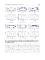
Fig. 7 shows the eye-diagram of electrical current and the corresponding PDF of the EDP at

the decision circuit input when Butterworth electrical filters are considered at the RX side.
This analysis allows assessing the impact of the group delay of electrical filters on the eye-
diagram and PDF of the EDP because the group delay of Butterworth electrical filters is
quite different from the one of Bessel electrical filters. The analysis of Fig. 7 shows that the
PDF of the EDP remains approximately Gaussian-distributed even when Butterworth
electrical filters are considered.

0 0.25 0.5 0.75 1
-0.6
-0.4
-0.2
0
0.2
0.4
0.6
t/T
s
Current [mA]

0 0.2 0.4 0.6 0.8 1
-0.6
-0.4
-0.2
0
0.2
0.4
0.6
t/T
s
Current [mA]

-1.25 -0.75 -0.25 0.25 0.75 1.25
-5
-4
-3
-2
-1
0
1
EDP
(/
π
)
log
10
PDF

-1.25 -0.75 -0.25 0.25 0.75 1.25
-5
-4
-3
-2
-1
0
1
EDP
(/
π
)
log

10
PDF

Fig. 7. Eye-diagram of electrical current and corresponding PDF of the EDP when a three
(left-hand side) or a five (right-hand side) pole Butterworth electrical filter with
GHz18=
e
B is considered at the RX side. An ideal RX is considered. Marks: MC simulation;
lines: GA estimated from the results of MC simulation.
The PDF of the EDP has also been assessed for 67% duty-cycle RZ-DQPSK signals for both
types of electrical filters, leading to similar conclusions to those presented in this section.
4. Gaussian approximation for equivalent differential phase
The GA consists in approximating a given PDF by a Gaussian PDF. In order to do so, the
mean and STD of the Gaussian PDF are set equal to the mean and STD of the PDF it is
approximating. The mean and STD of the EDP are derived in this section as a function of the
received DQPSK signal and PSD of optical noise at the RX input in order to obtain closed-
form expressions for the mean and STD of the EDP. Substituting eq. (2) in eq. (6) and setting
MZDI
Ttd −=
to simplify the expressions, we get:
Optical DQPSK Modulation Performance Evaluation

437

()
[]
{}
{}
(
[

)
]
{}
{}
⎭
⎬
⎫
∗
⎟
⎠
⎞
⎥
⎦
⎤
++++++ℜ+++
⎢
⎣
⎡
⎟
⎠
⎞
⎜
⎝
⎛
++++++ℜ++−
++++++
+++++++++
⎥
⎦
⎤

++ℜ++
⎢
⎣
⎡
⎟
⎠
⎞
⎜
⎝
⎛
++ℜ++
⎩
⎨
⎧
⎜
⎝
⎛
++++=Δ
⊥
⊥
⊥⊥
⊥
⊥
⊥⊥
)()()()()()(
)()()()()(
)()()()(
)()()()()()(
)()()()()(
)()()()()(

)()()()()()()()()()(arg)(
||
*
||
||
*
||
**
||
||
*
||
*
||
*
||
*
||
||
*
||
**
||
||
*
||
*
||
*),(
thtntntntsts

dndndndsds
R
edntndntn
dstndntsdsts
R
tntntntsts
dndndndsds
R
edntndntndstndntsdsts
R
t
e
j
j
QI
e
2
2
2
2
2
2
2
2
2
2
2
2
2
2

2
2
1
1
2
2
4
2
2
2
4
2
τττττ
τττττγ
ττττ
ττττττγ
γ
γφ
θ
θ
(7)
In order to obtain closed-form expressions for the mean and STD of the EDP, the
dependence of the EDP on noise is linearized. This approximation should lead to only very
small discrepancies in the mean and STD of the EDP as the EDP conditioned on the
transmitted symbols is approximately Gaussian-distributed. The linearization of the EDP is
performed expressing the argument of eq. (7) as an arctangent function. Thus, the several
beat terms of eq. (7) are decomposed in their real and imaginary parts. The several beat
terms can be written and defined as shown in eq. (14) and eq. (15) (Appendix 9.1). The time
dependence of the DQPSK signal and noise is omitted in order to simplify the notation. By
substituting the results shown in eqs. (14) and (15) in eq. (7) and by approximating the EDP

by a first order Taylor series we get

[]
(
[]
)
[]
(
[]
)
()
(
)
⎟
⎠
⎞
++++++
+++++−
++++
++++
++++
⎜
⎝
⎛
+++
+
+=Δ
⊥
⊥
⊥

⊥
⊥
⊥
⊥
⊥
,,
,,
||,,
,
||,,
,
,
,
||,
||,
,,||,,,,,,
,,
||,,
,,,,
,||,,
,
,
||,
,
,
),(
)arctan()(
t
d
t

t
d
d
t
d
t
t
dd
iiii
r
r
rr
iii
i
r
r
r
r
QI
e
nnnnnnsnnnsn
B
R
nnnnnnsnnnsn
B
R
nnnnsnsnc
nnnnsnsnc
R
nnnnsnsnc

nnnnsnsnc
R
k
k
kt
τ
τ
τ
τ
τ
τ
ττττ
τ
τ
ττ
γγγ
γγγ
γ
γφ
222
2
222
1
21
1
21
2
2
2
11

2
12
1
2
22
4
22
4
2
2
1
(8)
where

[]
[]
[]
[]
[][]
;)cos()sin(;)sin()cos(;/
;
44
)sin()cos(
2
)sin()cos(
2
;)sin()cos(
2
)sin()cos(
2

21
,
,
2
2
2
1
,,
21
,,
21
BAcBAcBAk
ssss
R
ssss
R
ssss
R
ssss
R
B
ssss
R
ssss
R
A
t
d
t
d

irir
riri
θθθθ
γγ
θθθθγ
θθθθγ
τ
τ
ττ
ττ
−=+==
+−++
⎟
⎠
⎞
⎜
⎝
⎛
−+−=
⎟
⎠
⎞
⎜
⎝
⎛
+++=
(9)
Advances in Lasers and Electro Optics

438

From eq. (8), the mean of the EDP is

{}
{}
(){}
{}
()
[]
{}
{}
(){}
{}
()
[]
{}{}
{}{}
()
{}{}
{}{}
[]
⎟
⎠
⎞
++++
+++−
++++
⎜
⎝
⎛
+++

+
+=
⊥⊥
⊥⊥
⊥⊥
⊥⊥
,,,,||,,||,,
,,||,||,
,,||,,,,||,,
,||,,||,
)arctan()(
tdtd
tdtd
iirr
iirr
nnnnnnnn
B
R
nnnnnnnn
B
R
nnnncnnnnc
R
nnnncnnnnc
R
k
k
kt
ττττ
ττττ

γγ
γγ
γ
γμ
EEEE
4
EEEE
4
EEEE
2
EEEE
2
1
22
2
22
1
12
2
12
1
2
(10)
Assuming uncorrelated noise over both polarization directions, i.e.,
()
()
()
yxyx
nnnnnnnn
,||,,||, ⊥⊥

= EEE , where x and y represent the real or imaginary part of noise-
noise beat terms and, as odd order moments of Gaussian processes with zero mean are null,
the variance of the EDP is given by:

[]
⎟
⎟
⎠
⎞
⎜
⎜
⎝
⎛
+
⎟
⎠
⎞
⎜
⎝
⎛
+
=
∑
=
−−
8
1
22
2
2

2
1
l
lASEASENlASEsN
k
k
t
,,,,
)(
σσσ
(11)
where
2
lASEsN ,, −
σ
and
2
lASEASEN ,, −
σ
are the contributions to the signal and noise-noise beat
variance, respectively, presented in Appendices 9.2 and 9.3. The variance of the EDP (eq.
(11)) is given by a lenghty expression. However, the evaluation of the several terms of eq.

0 5 10 15 20 25
0.13
0.17
0.21
0.25
0.29
Symbol number

STD of EDP
0 5 10 15 20 25
0.13
0.17
0.21
0.25
0.29
Symbol number
STD of EDP
0 5 10 15 20 25
0.13
0.17
0.21
0.25
0.29
Symbol number
STD of EDP

a) Ideal RX
b)
%2=
R
BΔf
c)
%40=
s
TΔ
τ

0 5 10 15 20 25

0.13
0.17
0.21
0.25
0.29
Symbol number
STD of EDP
0 5 10 15 20 25
0.13
0.17
0.21
0.25
0.29
Symbol number
STD of EDP
0 5 10 15 20 25
0.13
0.17
0.21
0.25
0.29
Symbol number
STD of EDP

d) R
1
=0.5 A/W, R
2
=1 A/W e) δT
MZDI

/T
s
=20%
f)
GHz20=
υ
Δ

Fig. 8. Standard deviation of the EDP. Only the STD of the EDP of some symbols transmitted
with two of the four nominal means (circles:
4
π
; squares:
43
π
−
) is shown in order to make
the figures clearer. Filled symbols: estimates from MC simulation results, obtained
considering 15000 noise realizations; empty symbols: estimates from the GA (eq. (11)).
Optical DQPSK Modulation Performance Evaluation

439
(11) is quite simple which makes the evaluation of the variance of the EDP of quite reduced
complexity. Furthermore, if no RX imperfections are considered, eq. (11) is quite simplified,
leading to the result shown in (Costa & Cartaxo, 2009). The derivation of the mean and
variance of EDP as a function of the received DQPSK signal and PSD of optical noise after
optical filtering is shown in (Costa & Cartaxo, 2009b)
Fig. 8 shows the STD of the EDP estimated using the results from MC simulation and the
GA (eq. (11)). Analysis of Fig. 8 shows that the estimates of the STD of the EDP obtained
using eq. (11) are quite accurate in presence of the majority of RX imperfections. The

accuracy of the estimates for the mean of the EDP, estimated using eq. (10), has also been
assessed showing that the mean of the EDP is always quite well estimated by eq. (10). The
quite good accuracy achieved in the estimation of the mean and STD of the EDP using
eqs. (10) and (11) shows that the linearization of the EDP leads only to very small
discrepancies on the evaluation of the mean and STD of the EDP and that the impact of
noise on the mean and STD of the EDP is correctly estimated.
5. Bit error probability computation by semi-analytical simulation method
A SASM for performance evaluation of DQPSK systems is proposed in this section. The
DQPSK signal at the RX input is evaluated by simulation. This permits evaluating the
impact of the transmission path, e.g. the nonlinear fiber transmission, the optical add-drop
multiplexer concatenation filtering, on the waveform of the DQPSK signal. A quaternary
deBruijn sequence with total length N
S
is used in the simulation. DeBruijn sequences include
all possible symbol sequences with a given length using the lower number of symbols
(Jeruchim et al., 2000). This characteristic is important since it assures that all possible cases
of inter-symbol interference (ISI) for a given sequence length occur. On the other hand, as
the EDP is approximately Gaussian–distributed when the optical noise is modelled as
AWGN at the RX input, the impact of noise on the DQPSK system performance is assessed
analytically.
As the precoding performed in the TX allows direct mapping of the bit sequence from the
TX input to the RX output, the overall BEP is given by
(
)
2
)()( QI
BEPBEPBEP += , where
),( QI
BEP is the BEP of each component of the DQPSK signal. In order to take accurately into
account the impact of ISI on the DQPSK system performance, separate Gaussian

distributions with different means and STDs are associated with each one of the transmitted
bits. This approach has already proved to be accurate to estimate the ISI impact on OOK
modulation (Rebola & Cartaxo, 2001). The BEP of each component of the DQPSK signal can
be seen as the mean of four BEPs associated with the four nominal means for the PDF of the
EDP. Thus, defining F as the EDP threshold level, with 0≥F , the BEP of the I and Q
components of the DQPSK signal is given by

⎟
⎟
⎟
⎟
⎠
⎞
⎜
⎜
⎜
⎜
⎝
⎛
⎥
⎥
⎦
⎤
⎢
⎢
⎣
⎡
+−
+
⎥

⎥
⎦
⎤
⎢
⎢
⎣
⎡
−
=
∑∑
±=
=
±=
=
s
n
n
n
s
n
n
n
N
a
n
,na
,na
N
a
n

,na
,na
s
QI
μFμF
N
BEP
43
1
4
1
2
erfc
2
erfc
2
1
ππ
σσ
),(
(12)
where erfc(x) is the complementary error function and
,na
n
μ and
,na
n
σ
are the mean and
STD of the EDP at the sampling time for the

n-th received symbol with nominal mean
n
a .
Advances in Lasers and Electro Optics

440
,na
n
μ and
,na
n
σ
are obtained from eq. (10) and eq. (11), respectively, by evaluating these
expressions at the sampling time and by associating each sampling time with each
transmitted symbol. The optimal threshold level of the EDP,
opt
F , is assessed by setting to
zero the derivative of eq. (12) with respect to
F, leading to the transcendental equation

∑∑
±=
=
±=
=
⎟
⎟
⎟
⎟
⎠

⎞
⎜
⎜
⎜
⎜
⎝
⎛
⎥
⎥
⎦
⎤
⎢
⎢
⎣
⎡
+−
−=
⎟
⎟
⎟
⎟
⎠
⎞
⎜
⎜
⎜
⎜
⎝
⎛
⎥

⎥
⎦
⎤
⎢
⎢
⎣
⎡
−
−
s
n
n
n
n
s
n
n
n
n
N
a
n
,na
,naopt
,na
N
a
n
,na
,naopt

,na
μFμF
43
1
2
4
1
2
2
1
exp
1
2
1
exp
1
ππ
σσσσ
(13)
that can be numerically solved using the Newton-Raphson method.
6. Accuracy of the SASM based on the GA for the EDP
In this section, the accuracy of the SASM for DQPSK system performance evaluation based
on the GA for the EDP is assessed. This analysis is performed comparing the results
obtained using eq. (12) with those obtained using MC simulation. A BEP = 10
-4
is set as the
target BEP mainly because MC simulation is much time consuming for lower BEP and the
use of forward error correction (FEC), such as Reed-Solomon codes, allows to achieve much
lower BEP at the expense of only a slight increase on the bit rate. The accuracy of the SASM
is firstly assessed in presence of RX imperfections. Then, the accuracy of the SASM is

assessed considering nonlinear fiber transmission. The bit error ratio estimates obtained
using MC simulation are only accepted after at least 100 errors occurring in each component
of the DQPSK signal. The threshold level is optimized and the time instant leading to higher
eye-opening in the absence of noise is chosen as sampling time. The TX and RX parameters
are the same as the ones considered in section 3, unless otherwise stated.
6.1 Accuracy of the SASM in presence of RX imperfections
When the ideal RX is considered, the MC simulation estimates that an OSNR of about 14 dB
is required to achieve BEP = 10
-4
. The SASM estimates a required OSNR of only about
13.8 dB. This small difference is attributed mainly to the difference between the GA for the
PDF of the EDP and its actual PDF. This conclusion results from having very good
agreement between the estimates of the mean and STD of the EDP obtained using eq. (10)
and eq. (11) with the corresponding ones obtained using MC simulation. Indeed, the SASM
leads to the correct required OSNR (14 dB) by increasing the STD of the EDP, calculated
using eq. (11), by only about 2.5%.
Fig. 9 shows the impact of several different RX imperfections on the OSNR penalty at
BEP = 10
-4
. The considered RX imperfections cover all expected values for each imperfection.
The impact of the RX imperfections on the DQPSK system performance has been assessed
by MC simulation and by SASM in order to assess the accuracy of the SASM. The analysis of
Fig. 9 shows that the SASM is quite accurate in presence of the majority of the typical RX
imperfections leading usually to a discrepancy on the OSNR penalty not exceeding 0.2 dB.
Among the cases analysed in Fig. 9, the higher discrepancies occur for high time-
misalignment of signals at the balanced detector input
()
%30>Δ T
τ
and for high

frequency detuning of the optical filters
()
GHz15>Δ
ν
. Indeed, the SASM leads to an
underestimation of the OSNR penalty in both cases that may attain about 0.5 dB.
Optical DQPSK Modulation Performance Evaluation

441
10 20 30 40 50
0
1
2
3
4

ε

[dB]
OSNR penalty [dB]
-2 -1 0 1 2
0
1
2
3
4
Δ
f/B
R
[%]

OSNR penalty [dB]
-50 -30 -10 10 30 50
0
1
2
3
4

Δ

τ
/T
s

[%]
OSNR penalty [dB]

a) MZDI extinction ratio
with
k=0.3
b) MZDI detuning
c) Time-misalignment of
signals at balanced
detector input
-0.5 -0.3 -0.1 0.1 0.3 0.5
0
1
2
3
4

k
OSNR penalty [dB]
-40 -20 0 20 40
0
1
2
3

δ
T
MZDI
/T
s

[%]
OSNR penalty [dB]
-20 -10 0 10 20
0
1
2
3
4

Δ

ν

[GHz]
OSNR penalty [dB]

d) Amplitude-imbalance of
balanced detector
e) MZDI delay error f) Optical filter detuning
Fig. 9. OSNR penalty at
4
10
−
=BEP
as a function of several different RX imperfections. Filled
circles: MC simulation; empty circles: SASM.

5 10 15 20 25 30 35 40
13
13.5
14
14.5
15
15.5
16
B
e

[GHz]
Required OSNR [dB
]

Fig. 10. Required OSNR at
4
10
−

=BEP as a function of the electrical filter type and
bandwidth, considering an ideal RX. Empty marks: SASM; filled marks: MC simulation.
Circles: five-pole Bessel electrical filter; squares: five-pole Butterworth electrical filter.
Fig. 10 illustrates the accuracy of the SASM when different bandwidths and types of
electrical filter are considered. Fig. 10 shows that the required OSNR is quite well estimated
independently of the type and bandwidth of the electrical filter. Indeed, the discrepancy of
the required OSNR does not usually exceed 0.2 dB. This small discrepancy is mainly
attributed to the difference between the GA for the PDF of the EDP and its actual PDF.
Fig. 10 shows also that the behavior of the required OSNR as a function of the electrical filter
bandwidth depends on the electrical filter type. The different behaviors illustrated in Fig. 10
for filter bandwidths around 12 GHz can be explained by observing the eye-opening.
Indeed, we find that the eye-opening is more reduced for
B
e
around 12.5 GHz than for B
e

around 11 GHz when the Butterworth electrical filter is used, which does not occur in case
of the Bessel electrical filter.
Advances in Lasers and Electro Optics

442
6.2 Accuracy of the SASM in presence of nonlinear fiber transmission
To reach long-haul cost-efficient transmission, as required in core networks, the fiber spans
should be quite long to reduce the number of required optical amplifiers. The power level at
the input of each span should also be as high as possible to achieve high OSNR. On the
other hand, when high power levels are used, the fiber nonlinearity imposes a severe power
penalty. Thus, a compromise between the optical power level and the power penalty
imposed by the fiber nonlinearity has to be accomplished. Standard single-mode fiber
(SSMF) is the transmission fiber type more commonly used in these networks. Despite its

many advantages, it introduces high distortion in the transmitted signal due to its high
dispersion. Thus, the use of dispersion compensation along the transmission path is
required.
In an ideal single-mode optical fiber, the two orthogonal states of polarization are
degenerated, i. e. they propagate with identical propagation constants (Iannone et al., 1998).
Thus, the input light-polarization would remain constant over the whole propagation
length. In reality, optical fibers may have a slightly elliptical core which leads to
birefringence, i. e. the propagation constants of the two orthogonal states of polarization
differ slightly. External perturbations such as stress, bending and torsion lead also to
birefringence (Hanik, 2002). Thus, the impact of fiber birefringence, group velocity
dispersion (GVD) and self-phase modulation (SPM) are considered to assess the accuracy of
the SASM in presence of nonlinear fiber transmission.
The MC simulation is performed by solving the coupled nonlinear Schrödinger propagation
equation, also known as the vector version of the nonlinear Schrödinger propagation
equation, instead of the scalar version of the nonlinear Schrödinger propagation equation, in
order to take into account the impact of fiber birefringence. However, the solution of the
coupled nonlinear Schrödinger propagation equation is much more complex than the one of
the scalar version (Iannone et al., 1998). Nevertheless, the split-step Fourier method, which
is usually used to solve the scalar version of the nonlinear Schrödinger propagation
equation, can be applied to its vector version when the so-called high-birefringence
condition (Iannone et al., 1998) is verified. In this case, the exponential term in the vector
version of the nonlinear Schrödinger propagation equation that depends on the
birefringence fluctuates rapidly and its effect tends to average out (Iannone et al., 1998). This
approximation is usually verified in single mode optical fibers and has been commonly used
in the literature where negligible loss of accuracy is usually achieved (Marcuse et al., 1997).
Furthermore, by choosing an adequate integration step, the coupling between the
polarization modes can be neglected when solving the propagation within a single step.
After each step, the eigenpolarizations are randomly rotated and a random phase shift is
added. A more detailed explanation of how the simulation of fiber nonlinear transmission is
performed can be found in (Iannone et al., 1998). In our MC simulation, the birefringence is

assumed constant over successive integration steps of 100 meters. The eigenpolarizations are
uniformly distributed over the birefringence axes and the phase shift, which corresponds to
π
2 over the beat length, has a Rician distribution with mean value
1
m210
−
⋅
π
. and variance
1
m2010
−
⋅
π
. (Carena et al., 1998).
The DQPSK system performance evaluation by the SASM requires assessing the DQPSK
noiseless waveform and PSD of optical noise at RX input after nonlinear fiber transmission.
The noiseless waveform of the DQPSK signal is assessed by performing noiseless
Optical DQPSK Modulation Performance Evaluation

443
transmission of the DQPSK signal using the scalar version of the nonlinear Schrödinger
equation, but with the fiber nonlinearity coefficient reduced by a 8/9 factor. Indeed, the
scalar version of the nonlinear Schrödinger propagation equation leads to similar results to
those of its vector version when it is solved with the fiber nonlinearity coefficient set to 8/9
of its real value (Carena et. al., 1998), (Hanik, 2002). The PSD of optical noise depends on the
polarization direction. Indeed, the AWGN approximation for optical noise at the RX input
over the same polarization direction as the DQPSK signal may be quite inaccurate when
nonlinear fiber transmission is considered. Indeed, when a strong signal (the DQPSK signal)

propagates along a transmission fiber, it creates a spectral region around itself where a small
signal (the optical amplifier’s ASE noise) experiences gain. This phenomenon is known as
parametric gain (Carena et al., 1998). Furthermore, the nonlinear phase noise due to the
amplitude-to-phase noise conversion effect arising from the interaction of the optical
amplifier’s ASE noise and the nonlinear Kerr effect must also be taken into account. The
evaluation of the parametric gain and nonlinear phase noise can be performed considering
the nonlinear fiber transmission of only one polarization direction but with the fiber
nonlinearity coefficient reduced by the 8/9 factor. This approximation allows evaluating the
PSD of optical noise after nonlinear fiber transmission over the DQPSK signal polarization
direction using the method proposed in (Demir, 2007). The method proposed in (Demir,
2007) evaluates the PSD of optical noise in a quite time efficient manner by deriving a linear
partial-differential equation for the noise perturbation. In order to do so, the nonlinear
Schrödinger equation is linearized around a continuous-wave signal. The AWGN
approximation for optical noise at RX input over the perpendicular polarization direction is
still quite accurate (Carena et al., 1998). Thus, the PSD of optical noise over the
perpendicular polarization direction is obtained by adding the individual ASE noise
contributions of each optical amplifier, each affected by the total gain from the optical
amplifier till the RX.

Span 1
DQPSK
TX
P
in
P
in
P
in
EDFA
EDFA

DCF
EDFA
EDFA
P
DCF
DCF
DQPSK
RX
SSMF
SSMF
P
DCF
P
RX
=0 dBm
Span N
sp

Fig. 11. Scheme of the DQPSK transmission system.
Fig. 11 shows the schematic configuration of the DQPSK transmission system. The total link
is composed by
N
sp
spans, with N
sp
=20. Each span is composed by 100 km of SSMF followed
by a double-stage erbium-doped fiber amplifier (EDFA). Dispersion compensating fibers
(DCFs) are used for total compensation of the dispersion accumulated in the SSMF of each
span. To assure that all DCFs operate nearly in linear regime, the power level denoted by
P

DCF
is imposed at the DCFs input. The average power level at the input of each SSMF is
denoted by
P
in
. The total gain of both EDFAs’ stages compensates for the power loss in each
span, except in the last span. In this case, the second stage EDFA is used to impose a power
level of 0 dBm at the RX input. The SSMF has an attenuation parameter of 0.21 dB/km, a
dispersion parameter of 17 ps/nm/km, an effective core area of 80 μm
2
and a nonlinear
index-coefficient of 0.025 nm
2
/W. The EDFA’s noise figure is 7 dB. The dispersion
parameter of the DCF is -100 ps/nm/km and its attenuation parameter depends on the
Advances in Lasers and Electro Optics

444
transmission scenario that is being considered. Indeed, in order to keep the BEP high
enough to perform MC simulation in a reasonable amount of time and, as 33% duty-cycle
RZ-DQPSK pulses show better performance than NRZ-DQPSK pulses, the attenuation
parameter of DCF is 0.5 dB/km when NRZ-DQPSK pulses are considered and 0.6 dB/km
when 33% duty-cycle RZ-DQPSK pulses are considered. Furthermore,
dBm8−=
DCF
P
when NRZ-DQPSK pulses are considered and
dBm12−=
DCF
P

when 33% duty-cycle RZ-
DQPSK pulses are considered.

-5 -3 -1 1 3 5
-5
-4.5
-4
-3.5
-3
-2.5
-2
P
in

[dBm]
log
10

BEP

-5 -3 -1 1 3 5
-5
-4.5
-4
-3.5
-3
-2.5
-2
P
in

[dBm]
log
10

BEP

Fig. 12. Performance of NRZ-DQPSK (left) and 33% duty-cycle RZ-DQPSK (right) for the
transmission system of Fig. 11. Filled circles: MC simulation; empty circles: SASM.
Fig. 12 shows the performance of DQPSK modulation in presence of nonlinear fiber
transmission. When NRZ-DQPSK signals are considered (figure on the left), a good accuracy
is achieved both when ASE noise is the main transmission impairment (lower power levels)
and when the transmission is mainly limited by fiber nonlinearity (higher power levels).
This result leads to the conclusion that methods for DQPSK system performance evaluation
based on the GA for the EDP lead to quite good accuracy even in presence of nonlinear fiber
transmission when NRZ-DQPSK signals are considered. The analysis of the figure on the
right-hand side, where the transmission of a 33% duty-cycle RZ-DQPSK signal is
considered, shows that the SASM estimates the performance of the DQPSK system quite
accurately when ASE noise is the main impairment. However, the accuracy of the SASM
tends to decrease with the increase of the impact of the fiber nonlinearity. This loss of
accuracy is not a consequence of the loss of accuracy of the GA for the EDP. Indeed, quite
good accuracy is achieved when the mean and STD of the EDP are estimated from the
results of MC simulation. The decrease of accuracy of the SASM is a consequence of the
inaccuracy in the evaluation of the PSD of optical noise. Indeed, the linearization of the
nonlinear Schrödinger equation around a continuous-wave signal does not provide an
acceptable description of noise statistics when 33% duty-cycle RZ-DQPSK signals are
transmitted and the impact of fiber nonlinearity is important.
Computation time gains of about 15000 times have been achieved by the SASM when
compared with MC simulation for
BEP = 10

-4
.
7. Conclusion and work in progress
The performance evaluation of simulated optical DQPSK modulation has been analysed.
The EDP of DQPSK signals is approximately Gaussian-distributed. Thus, a SASM for
DQPSK systems performance evaluation based on the GA has been proposed. The SASM
relies on the use of the closed-form expressions derived for the mean and STD of the EDP
Optical DQPSK Modulation Performance Evaluation

445
for assessing the performance of the DQPSK system in a time-efficient manner. Quite good
agreement between MC simulation and the results of the SASM is usually achieved, even in
presence of RX imperfections and nonlinear fiber transmission. Indeed, although the SASM
leads usually to an underestimation of the required OSNR of about 0.2 dB, the discrepancy
of the OSNR penalty at
BEP = 10
-4
is usually below 0.2 dB for the majority of the typical RX
imperfections.
Several subjects on the performance evaluation of DQPSK signals using the GA for the EDP
are still to be addressed. Indeed, the evaluation of the PSD of optical noise at RX input, after
nonlinear transmission, admitting a modulated signal and the accuracy improvement of the
SASM achieved by using the more accurate description for the PSD of optical noise is still to
be performed. The validation of the SASM for
BEP around 10
-12
and the proposal of a
scheme for evaluating the EDP experimentally are also still to be addressed.
8. Acknowledgments
This work was supported in part by Fundação para a Ciência e a Tecnologia from Portugal

under Ph.D. contract SFRH/BD/42287/2007.
9. Appendix
9.1 List of beat terms at decision circuit Input
The current and the EDP at the decision circuit input are given as a function of the following
beat terms:

(
)
[]
()
()
[]
()
()
[]
()
()
[]
()
()
[]
()
()
{}
()
()
()
{}
()
()

()
()
⊥⊥⊥⊥
⊥⊥⊥⊥
⊥⊥
⊥⊥⊥⊥⊥⊥⊥⊥⊥⊥
≡∗+=∗
≡∗+=∗
≡∗+=∗
≡∗+=∗ℜ
≡∗+=∗
≡∗+=∗
≡∗+=∗ℜ
≡∗+=∗
+≡
∗−++=∗
+≡
∗−++=∗
+≡∗−++=∗
+≡∗−++=∗
+≡∗−++=∗
,,,
,,,
||,||,||,||
||,||,
*
||
||,||,||,||
||,||,
*

||
,,
,,,,,,,,
*
||,||,
||,||,||,||,||,||,||,||,
*
||||
,,||,||,||,||,
*
||
,,||,||,||,||,
*
||
*
)()()()(|)(|
)()()()(|)(|
)()()()(|)(|
)()()()()()()()(
)()()()(|)(|
)()()()(|)(|
)()()()()()()()(
)()()()(|
)(|
)()()()()()()()()()()()(
)()()()()()()()()()()()(
)()()()()()()()()()()()(
)()()()()()()()()()()()(
)(
)()()()()()()()()()()(

teire
deire
teire
teiirre
deire
teire
deiirre
deire
ir
eirriiirre
ir
eirriiirre
ireirriiirre
ireirriiirre
ireirriii
rre
nnthtntnthtn
nnthdndnthdn
nnthtntnthtn
snthtntstntsthtnts
nnthdndnthdn
ssthtststhts
snthdndsdndsthdnds
ssthdsdsthds
jnn
nn
thdntndntnjdntndntnthdntn
jnnnn
thdntndntnjdntndntnthdntn
jsnsnthdstndstnjdstndstnthdstn

jsnsnthdntsdntsjdntsdnts
thdnts
jssssthdstsdstsjdstsdststhdsts
222
222
222
222
222
222
22
11
(14)
Advances in Lasers and Electro Optics

446
and, similarly:


(
)
(
)
() ( )
()
{}
{}
⊥⊥
⊥⊥
⊥⊥⊥⊥
≡∗+

≡∗+≡∗+
≡∗++ℜ≡∗+
≡∗+≡∗++ℜ
≡∗++≡∗++
+≡∗+++≡∗++
+≡∗+++≡∗++
,,
,,,||,||
,
*
||,||,||
,,
*
||
,,,,,
*
,||,,||,
*
||||,,,,
*
||
,,,,
*
||,,
*
)(|)(|
)(|)(|;)(|)(|
)()()(;)(|)(|
)(|)(|;)()()(
)(|)(|;)()()(

)()()(;)()()(
)()()(;)()()(
te
dete
tede
tede
deire
ireire
ireire
nnthtn
nnthdnnnthtn
snthtntsnnthdn
ssthtssnthdnds
ssthdsjnnnnthdntn
jnnnnthdntnjsnsnthdstn
jsnsnthdntsjssssthdsts
τ
ττ
ττ
ττ
τττ
ττττ
ττττ
τ
ττ
τττ
τττ
τττ
ττττ
ττττ

2
22
2
2
2
22
11
(15)
9.2 Contributions to the signal-noise beat variance
The variance of the signal-noise beat may be separated in several contributions. To illustrate
the impact of RX imperfections, the contributions to the signal-noise beat variance of ideal
RX, shown in (Costa & Cartaxo, 2009b), are used as reference. Thus, we find that the
()
{
}
{
}
()
{
}
(
)
2
2
21
2
1
2
2
EE2E

r
rr
r
snsnsnsnc
,
,,
,
++ contribution to the signal-noise beat variance
results from


()
{}
{}
()
{}
(
)
()
{}
{}()
{}()
{}{}{}{}()
rrrrrrrr
rrrr
r
rr
rASEsN
snsnsnsnsnsnsnsnc
RR

snsnsnsnc
R
snsnsnsnc
R
,,,,,,,,,,,,
,,,,,,,,
,
,,
,,,
22122111
2
2
21
2
2
221
2
1
2
2
2
2
2
2
2
21
2
1
2
2

2
1
22
1
EEEE
2
EE2E
4
EE2E
4
ττττ
ττττ
γ
γ
γσ
++++
+++
++=
−
(16)

by considering an ideal RX. Similarly, the
()
{
}
{
}
()
{
}

(
)
2
2
21
2
1
2
1
EE2E
i
ii
i
snsnsnsnc
,
,,
,
++ and
{
}
{
}
{
}
{
}
(
)
iriririr
snsnsnsnsnsnsnsncc

,,,,,,,, 2221121121
EEEE2 +++ contributions to the signal-noise
beat variance result from


()
{}
{}
()
{}
(
)
()
{}
{}()
{}()
{}{}{}{}()
iiiiiiii
iiii
i
ii
iASEsN
snsnsnsnsnsnsnsnc
RR
snsnsnsnc
R
snsnsnsnc
R
,,,,,,,,,,,,
,,,,,,,,

,
,,
,,,
22122111
2
1
21
2
2
221
2
1
2
1
2
2
2
2
2
21
2
1
2
1
2
1
22
2
EEEE
2

EE2E
4
EE2E
4
ττττ
ττττ
γ
γ
γσ
++++
+++
++=
−
(17)

and
Optical DQPSK Modulation Performance Evaluation

447

{}{}{}{}()
{}{}{}{}()
{}{}{}{}()
{}{}{}{}()
iriririr
iriririr
iriririr
iriririrASEsN
snsnsnsnsnsnsnsncc
R

snsnsnsnsnsnsnsncc
RR
snsnsnsnsnsnsnsncc
RR
snsnsnsnsnsnsnsncc
R
,,,,,,,,,,,,,,,,
,,,,,,,,,,,,
,,,,,,,,,,,,
,,,,,,,,,,
2221121121
2
2
2
2212211121
21
2
2221121121
21
2
2221121121
2
1
22
3
EEEE
2
EEEE
2
EEEE

2
EEEE
2
ττττττττ
ττττ
ττττ
γ
γ
γ
γσ
++++
++++
++++
+++=
−
(18)
respectively, when the ideal RX is considered. Other contributions to the signal-noise beat
variance arise from the imperfections of the RX and are cancelled when the ideal RX is
considered. These contributions are:

{}{}{}{}
()
{}{}{}{}
()
trdrtrdr
trdrtrdrASEsN
snsnsnsnsnsnsnsnc
B
R
snsnsnsnsnsnsnsnc

B
RR
,,,,
,,,,,,,,,,
22
2
11
2
2
2
1
22
2
11
2
2
21
2
4
EEEE
2
EEEE
2
+++−
+++=
−
γγγ
γγγσ
ττττ
(19)

{}{}{}{}
()
{}{}{}{}
()
tiditidi
tiditidiASEsN
snsnsnsnsnsnsnsnc
B
R
snsnsnsnsnsnsnsnc
B
RR
,,,,
,,,,,,,,,,
22
2
11
2
1
2
1
22
2
11
2
1
21
2

5
EEEE
2
EEEE
2
+++−
+++=
−
γγγ
γγγσ
ττττ
(20)


{}{}{}{}
()
{}{}{}{}
()
trdrtrdr
trdrtrdrASEsN
snsnsnsnsnsnsnsnc
B
RR
snsnsnsnsnsnsnsnc
B
R
,,,,,,,,
,,,,,,,,,,,,,,
22
2

11
2
2
21
22
2
11
2
2
2
2
2
6
EEEE
2
EEEE
2
ττττ
ττττττττ
γγγ
γγγσ
+++−
+++=
−
(21)


{}{}{}{}
()
{}{}{}{}

()
tiditidi
tiditidiASEsN
snsnsnsnsnsnsnsnc
B
RR
snsnsnsnsnsnsnsnc
B
R
,,,,,,,,
,,,,,,,,,,,,,,
22
2
11
2
1
21
22
2
11
2
1
2
2
2
7
EEEE
2
EEEE
2

ττττ
ττττττττ
γγγ
γγγσ
+++−
+++=
−
(22)


()
{}
{}()
{}
(
)
()
{}
{}()
{}
(
)
{ }{}{}{}
()
.
,,,,
,,,,
,,
ttdttddd
ttdd

ttddASEsN
snsnsnsnsnsnsnsn
B
RR
snsnsnsn
B
R
snsnsnsn
B
R
ττττ
ττττ
γγγ
γγ
γγσ
EEEE
2
EE2E
4
EE2E
4
224
2
21
2
2
2
4
2
2

2
2
2
2
4
2
2
1
2
8
+++−
+++
++=
−
(23)
Advances in Lasers and Electro Optics

448
9.3 Contributions to the noise-noise beat variance
The variance of the noise-noise beat may be separated in several contributions. To illustrate
the impact of RX imperfections, the contributions to the noise-noise beat variance of ideal
RX, shown in (Costa & Cartaxo, 2009b), are used as reference. Thus, we find that the
()
{
}
{}
()
{
}
{}

(
)
rrrr
nnnnnnnnc
,,||,||, ⊥⊥
−+−
2
2
2
2
2
2
EEEE contribution to the noise-noise beat variance
results from


()
{}
{}
()
{}
{}
(
)
()
{}
{}
()
{}
{}

(
)
{}{}{}
{}{}{}
()
rrrrrrrr
rrrr
rrrrASEASEN
nnnnnnnnnnnnnnnnc
RR
nnnnnnnnc
R
nnnnnnnnc
R
,,,,,,||,,||,||,,||,
,,,,||,,||,,
,,||,||,,,
⊥⊥⊥⊥
⊥⊥
⊥⊥−
−+−+
−+−+
−+−=
ττττ
ττττ
γ
γ
γσ
EEEEEE
2

EEEE
4
EEEE
4
2
2
21
2
2
2
2
2
2
2
2
2
2
2
2
2
2
2
2
2
1
22
1
(24)

by considering an ideal RX. Similarly, the

()
{
}
{}
()
{
}
{}
(
)
iiii
nnnnnnnnc
,,||,||, ⊥⊥
−+−
2
2
2
2
2
1
EEEE
and
{
}
{
}
{
}
{
}

{
}
{
}
(
)
iriririr
nnnnnnnnnnnnnnnncc
,,,,||,||,||,||, ⊥⊥⊥⊥
−+− EEEEEE2
21
contributions to the
noise-noise beat variance result from


()
{}
{}
()
{}
{}
(
)
()
{}
{}
()
{}
{}
()

{}{}{}
{}{}{}
()
iiiiiiii
iiii
iiiiASEASEN
nnnnnnnnnnnnnnnnc
RR
nnnnnnnnc
R
nnnnnnnnc
R
,,,,,,,||,||,,||,||,
,,,,,||,,||,
,,||,||,,,
⊥⊥⊥⊥
⊥⊥
⊥⊥−
−+−+
−+−+
−+−=
ττττ
ττττ
γ
γ
γσ
EEEEEE
2
EEEE
4

EEEE
4
2
1
21
2
2
2
2
2
2
1
2
2
2
2
2
2
2
2
1
2
1
22
2
(25)

and

{}{}{}
{}{}{}
()
{}{}{}
{}{}{}
()
{}{}{}
{}{}{}
()
{}{}{}
{}{}{}
()
iriririr
iriririr
iriririr
iriririrASEASEN
nnnnnnnnnnnnnnnncc
R
nnnnnnnnnnnnnnnncc
RR
nnnnnnnnnnnnnnnncc
RR
nnnnnnnnnnnnnnnncc
R
,,,,,,,,||,,||,,||,,||,,
,,,,,,||,,||,||,,||,
,,,,,,||,||,,||,||,,
,,,,||,||,||,||,,,
⊥⊥⊥⊥
⊥⊥⊥⊥

⊥⊥⊥⊥
⊥⊥⊥⊥−
−+−+
−+−+
−+−+
−+−=
ττττττττ
ττττ
ττττ
γ
γ
γ
γσ
EEEEEE
2
EEEEEE
2
EEEEEE
2
EEEEEE
2
21
2
2
2
21
21
2
21
21

2
21
2
1
22
3
(26)

respectively, when the ideal RX is considered. Other contributions to the noise-noise beat
variance arise from the imperfections of the RX and are cancelled when the ideal RX is
considered. These contributions are:
Optical DQPSK Modulation Performance Evaluation

449

{}{}{}
{}{}{}
[]
(
{}{}{}
{}{}{}
)
{}{}{}
{}{}{}
[]
(
{}{}{}
{}{}{}
)
⊥⊥⊥⊥

⊥⊥⊥⊥
⊥⊥⊥⊥
⊥⊥⊥⊥−
−+−+
−+−−
−+−+
−+−=
,,,,||,||,||,||,
,,,,||,||,||,||,
,,,,,,||,,||,||,,||,
,,,,,,||,,||,||,,||,,,
trtrtrtr
drdrdrdr
trtrtrtr
drdrdrdrASEASEN
nnnnnnnnnnnnnnnn
nnnnnnnnnnnnnnnnc
B
R
nnnnnnnnnnnnnnnn
nnnnnnnnnnnnnnnnc
B
RR
EEEEEE
EEEEEE
4
EEEEEE
EEEEEE
4
2

2
2
1
2
2
21
2
4
γγ
γγσ
ττττ
ττττ
(27)



{}{}{}
{}{}{}
[]
(
{}{}{}
{}{}{}
)
{}{}{}
{}{}{}
[]
(
{}{}{}
{}{}{}
)

⊥⊥⊥⊥
⊥⊥⊥⊥
⊥⊥⊥⊥
⊥⊥⊥⊥−
−+−+
−+−−
−+−+
−+−=
,,,,||,||,||,||,
,,,,||,||,||,||,
,,,,,,||,,||,||,,||,
,,,,,,||,,||,||,,||,,,
titititi
didididi
titititi
didididiASEASEN
nnnnnnnnnnnnnnnn
nnnnnnnnnnnnnnnnc
B
R
nnnnnnnnnnnnnnnn
nnnnnnnnnnnnnnnnc
B
RR
EEEEEE
EEEEEE
4
EEEEEE
EEEEEE
4

2
1
2
1
2
1
21
2
5
γγ
γγσ
ττττ
ττττ
(28)



{}{}{}
{}{}{}
[ ]
(
{}{}{}
{}{}{}
)
{}{}{}
{}{}{}
[]
(
{}{}{}
{}{}{}

)
⊥⊥⊥⊥
⊥⊥⊥⊥
⊥⊥⊥⊥
⊥⊥⊥⊥−
−+−+
−+−−
−+−+
−+−=
,,,,,,||,||,,||,||,,
,,,,,,||,||,,||,||,,
,,,,,,,,||,,||,,||,,||,,
,,,,,,,,||,,||,,||,,||,,,,
trtrtrtr
drdrdrdr
trtrtrtr
drdrdrdrASEASEN
nnnnnnnnnnnnnnnn
nnnnnnnnnnnnnnnnc
B
RR
nnnnnnnnnnnnnnnn
nnnnnnnnnnnnnnnnc
B
R
EEEEEE
EEEEEE
4
EEEEEE
EEEEEE

4
2
2
21
2
2
2
2
2
6
ττττ
ττττ
ττττττττ
ττττττττ
γγ
γγσ
(29)



()
{}
{}
()
{}
{}
[]
(
{}{}{}
{}{}

{}
[]
()
{}
{}
()
{}
{}
)
()
{}
{}
()
{}
{}
[]
(
{}{}{}
{}{}
{}
[ ]
()
{}
{}
()
{}
{}
)
{}{}{}
{}{}{}

[]
(
{}{}{}
{}{}
{}
[]
{}{}{}
{}
{}
{}
[]
{}{}{}
{}{}{}
)
⊥⊥⊥⊥
⊥
⊥
⊥
⊥
⊥
⊥
⊥
⊥
⊥⊥⊥⊥
⊥⊥
⊥
⊥
⊥
⊥
⊥⊥

⊥⊥
⊥
⊥
⊥
⊥
⊥⊥
−
−+−+
−+−+
−+−+
−+−−
−+−+
−+−+
−+−+
−+−+
−+−+
−+−=
,,,,,,
||,,||,||,,||,
,,
,
,,
,
||,,||,||,,||,
2
,,
,
,,
,||,,||,||,,||,
2

,,,,,,||,,||,||,,||,
4
2
21
,,
2
2
,,
||,,
2
2
||,,
,,
,,
,,
,,||,,||,,||,,
||,,
2
,,
2
2
,,||,,
2
2
||,,
4
2
2
2
,

2
2
,
||,
2
2
||,
,
,
,
,||,||,||,||,
2
,
2
2
,||,
2
2
||,
4
2
2
1
2
7,,
EEEEEE
EEEEEE
EEEEEE
EEEEEE
8

EEEE
EEEEEE2
EEEE
16
EEEE
EEEEEE2
EEEE
16
tttt
tttt
d
t
d
t
dtdt
t
d
t
dtdtd
dddddddd
tt
tt
t
d
t
dtdtd
dddd
tt
tt
t

d
t
dtdtd
dddd
ASEASEN
nnnnnnnnnnnnnnnn
nnnnnnnnnnnnnnnn
nnnnnnnnnnnnnnnn
nnnnnnnnnnnnnnnn
B
RR
nnnnnnnn
nnnnnnnnnnnnnnnn
nnnnnnnn
B
R
nnnnnnnn
nnnnnnnnnnnnnnnn
nnnnnnnn
B
R
ττ
ττ
ττττ
ττ
ττ
ττττ
ττ
ττ
τ

τ
τ
τττττ
ττττ
γ
γ
γ
γ
γ
γ
γσ
(30)
Advances in Lasers and Electro Optics

450

{}{}{}
{}
{}
{}
[ ]
(
{}{}{}
{}{}{}
)
{}{}{}
{}
{}
{}
[]

(
{}{}{}
{}{}{}
)
⊥⊥⊥⊥
⊥
⊥
⊥
⊥
⊥⊥⊥⊥
⊥
⊥
⊥
⊥−
−+−+
−+−−
−+−+
−+−=
,,,,,,
||,||,,||,||,,
,
,,
,
,,
||,||,,||,||,,
2
1
21
,,,,,,,,
||,,||,,||,,||,,

,,
,,
,,
,,
||,,||,,||,,||,,
2
1
2
2
2
8,,
EEEEEE
EEEEEE
4
EEEEEE
EEEEEE
4
titi
titi
d
i
d
i
didi
titi
titi
d
i
d
i

didi
ASEASEN
nnnnnnnnnnnnnnnn
nnnnnnnnnnnnnnnnc
B
RR
nnnnnnnnnnnnnnnn
nnnnnnnnnnnnnnnnc
B
R
ττ
ττ
ττ
ττ
ττττ
ττττ
τ
τ
τ
τ
ττττ
γγ
γγσ
(31)

9.4 List of acronyms
AWGN – Additive white Gaussian noise
BEP – Bit error probability
DCF – Dispersion compensating fiber
DPSK – Differential phase-shift-keying

DQPSK – Differential quadrature phase-shift-keying
EDFA – Erbium doped fiber amplifier
EDP- Equivalent differential phase
GA- Gaussian approximation
GVD – Group velocity dispersion
I – In-phase
MC - Monte-Carlo
MZDI – Mach-Zehnder delay interferometer
NRZ – Non-return-to-zero
OOK – On-off keying
OSNR - Optical signal-to-noise ratio
PDF – Probability density function
PIN - Positive-intrinsic-negative photodetector
PSD – Power spectral density
Q – Quadrature
RX – Receiver
RZ – Return-to-zero
SASM - Semi-analytical simulation method
SPM – Self-phase modulation
SSMF - Standard single-mode fiber
STD – Standard deviation
TX - Transmitter
Optical DQPSK Modulation Performance Evaluation

451
10. References
Bosco, G. & Poggiolini, P. (2006). On the joint effect of receiver impairments on direct-
detection DQPSK systems, IEEE/OSA J. Lightwave Technol., vol. 24, no. 3, Mar. 2006,
pp. 1323-1333.
Carena, C., Curri, V. et al. (1998). On the joint effects of fiber parametric gain and

birefringence and their influence on ASE noise, IEEE/OSA J. Lightwave Technol., vol.
16, no. 7, Jul. 1998, pp. 1149-1157.
Costa, N. & Cartaxo, A. (2007). BER estimation in DPSK systems using the differential phase
Q taking into account the electrical filtering influence, IEEE Proc. Intern. Microwave
and Optoelectron. Conf., Salvador, Brazil, Oct. 2007, pp. 337-340.
Costa, N. & Cartaxo, A. (2009). Novel semi-analytical method for BER evaluation in
simulated optical DQPSK systems, IEEE Photon. Technol. Lett., vol. 21, no. 7, Apr.
2009, pp. 447-449.
Costa, N. & Cartaxo, A. (2009b). Optical DQPSK system performance evaluation using
equivalent differential phase in presence of receiver imperfections, IEEE/OSA J.
Lightwave Technol., submitted paper.
Demir, A. (2007). Nonlinear phase noise in optical-fiber-communication systems, J.
Lightwave Technol., vol. 25, no. 8, Aug. 2007, pp. 2002-2032.
Hanik, N. (2002). Modelling of nonlinear optical wave propagation including linear mode-
coupling and birefringence, Optics Communications, vol. 214, Dec. 2002, pp. 207-230.
Ho, K P. (2005). Phase-Modulated Optical Communication Systems, Springer, ISBN-13: 978-0-
387-24392-4, United States of America, 2005.
Ip, E. & Kahn, J. (2006). Power spectra of return-to-zero optical signals, IEEE/OSA J.
Lightwave Technol., vol. 24, no. 3, Mar. 2006, pp. 1610-1618.
Iannone, E., Matera, F. et al. (1998). Nonlinear Optical Communication Networks, John Wiley &
Sons, ISBN: 0-471-15270-6, United States of America, 1998.
Jeruchim, M., Balaban, P. & Shanmugan, K. (2000). Simulation of Communication Systems -
Modelling, Methodology and Techniques, Kluwer Academic/Plenum Publishers, ISBN:
0-306-46267-2, United States of America, 2000.
Marcuse, D., Menyuk, C. R. & Way, P. K. (1997). Application of the Manakov-PMD equation
to studies of signal propagation in optical fibers with randomly varying
birefringence, IEEE/OSA J. Lightwave Technol., vol. 15, no. 9, Sept. 1997, pp. 1735-
1746.
Morita, I. & Yoshikane, N. (2005). Merits of DQPSK for ultrahigh capacity transmission,
Proc. IEEE LEOS Annual Meeting, Sydney, Australia, Oct. 2005, paper We5.

Rebola, J. L. & Cartaxo, A. (2001). Gaussian approach for performance evaluation of
optically preamplified receivers with arbitrary optical and electrical filters, IEE
Proc. Optoelectron., vol. 148, no. 3, Jun. 2001, pp. 135-142.
Winzer, P. J. & Essiambre, R J. (2006). Advanced modulation formats for high-capacity
optical transport networks, IEEE/OSA J. Lightwave Technol., vol. 24, no. 12, Dec.
2006, pp. 4711-4728.
Winzer, P. J., Raybon, G. et al. (2008). 100-Gb/s DQPSK transmission: from laboratory
experiments to field trials, IEEE/OSA J. Lightwave Technol., vol. 26, no. 20, Oct. 2008,
pp. 3388-3402.
Advances in Lasers and Electro Optics

452
Xu, C., Liu, X. & Wei, X. (2004). Differential phase-shift keying for high spectral efficiency
optical transmissions, IEEE J. Select. Topics in Quantum Electron., vol. 10, no. 2,
Mar./Apr. 2004, pp. 281-293.
20
Fiber-to-the-Home System
with Remote Repeater
An Vu Tran, Nishaanthan Nadarajah and Chang-Joon Chae
Victoria Research Laboratory, NICTA Ltd.
Level 2, Building 193, Electrical & Electronic Engineering
University of Melbourne, VIC. 3010,
Australia
1. Introduction
In the last few years, there has been rapid deployment of fixed wireline access networks
around the world based on fiber-to-the-home (FTTH) architecture. Passive optical network
(PON) is emerging as the most promising FTTH technology due to the minimal use of
optical transceivers and fiber deployment, and the use of passive outside plant (OSP) (Dixit,
2003; Kettler et al., 2000; Kramer et al., 2002). However, large scale PON deployment is to
some degree still limited by the high cost of the customer’s optical network unit (ONU),

which contains a costly laser transmitter. The active optical network (AON) architecture is
one potential solution that can reduce the ONU cost by utilizing low-cost vertical cavity
surface emitting laser (VCSEL) based transmitters. However, this system requires an
Ethernet switch at the remote node, which is expensive in terms of cost and maintenance,
and needs additional transceiver per customer. Another drawback of traditional PON
systems is that it has a split ratio limitation of 1:32, which makes it harder and much more
expensive to upgrade the network once more customers are connected.
In this book chapter, a FTTH system to reduce the ONU transmitter cost based on the use of
an upstream repeater at the remote node is reported. The repeater consists of standard PON
transmitter and receiver and therefore, does not significantly increase the overall system
cost. Moreover, by utilizing bidirectional Ethernet PON (EPON) transceiver modules to
regenerate the downstream signals as well as the upstream signals, we are able to extend the
feeder fiber reach to 60 km and split ratio of the FTTH system to 1:256. The repeater-based
system is demonstrated for both standard EPON-based FTTH and extended FTTH systems
and shows insignificant performance penalty.
In order to achieve higher user count and longer range coverage in the access network, the
repeater-based FTTH system can be cascaded in series. This will result in a lower network
installation cost per customer, especially when FTTH take-up rate is low. In this chapter, we
also investigate the jitter performance of cascaded repeater-based FTTH architectures via a
recirculating loop. Our demonstration shows that we can achieve up to 4 regeneration loops
with insignificant penalty and the total timing jitter is within the IEEE EPON standard
requirement.
With the presence of the active repeater at the remote node of a FTTH system, we can
provide additional functionalities for the network including video service delivery and local
Advances in Lasers and Electro Optics

454
internetworking. These systems will be investigated and presented in this chapter together
with an economic study of the repeater-based FTTH system compared with other
technologies.

2. FTTH system with remote repeater
A schematic of the proposed FTTH architecture with an upstream repeater is shown in Fig. 1
(Tran et al., 2006b). In this architecture, a conventional 1×N star coupler (SC) is replaced by a
2×N SC. One arm of the SC on the optical line terminal (OLT) side is connected to the
remote repeater, which could be at the same location as the SC or at a different location for
access to commercial power lines with a battery back-up. The other arm of the SC is to
transmit downstream signals through the SC and bypass the remote repeater. An isolator is
installed on this downstream path to prevent upstream signals from entering. The
downstream and upstream signals are separated/combined using a coarse wavelength
division multiplexer (CWDM). The upstream signals can be 2R or 3R regenerated at the
remote repeater using a burst-mode receiver (BMR), a burst-mode transmitter (BMT) and/or
a clock-data recovery (CDR) module. The BMR and BMT can have the same specification as
the OLT-receiver and ONU-transmitter, respectively. The CDR should be able to recover the
clock and data at a rate of the PON system.

SMF
2xN
SC
OLT
BMT
λ
d
λ
u
CWDM
BMR
ONU
ONU
λ
u

λ
d
λ
u
Remote Repeater
CDR
Passive OSP

Fig. 1. FTTH system with upstream repeater.
The use of an upstream repeater provides the opportunity for much lower cost
implementation of ONU using low power and low cost optical transmitters, such as
0.8/1.3/1.55 μm VCSEL-based transmitters. The ONU transmitters will now need much less
output power (up to 10 dB lower) than standard PON system due to feeder fiber and OLT
coupling losses. The use of simple and standard PON transceivers at the repeater
significantly saves cost, maintenance expenses and power compared to an Ethernet switch
as in the case of the AON architecture. Our proposed technique uses the conventional PON
fiber plant for both downstream and upstream transmissions. Moreover, it is compatible
with any existing media access control (MAC) protocols in the conventional PON systems as
the repeater simply regenerates the upstream signals without any modification to the
internal frame structure. Another advantage of our proposed FTTH system is that the
downstream signals need not to be regenerated at the remote repeater and as a result,
Fiber-to-the-Home System with Remote Repeater

455
downstream channel can be upgraded without any change in the repeater allowing
broadcast services to be transmitted transparently through the 1.55 μm wavelength window.
PON transmitter and receiver are usually commercially available as a single bidirectional
transceiver (TRX) unit. By utilizing the bidirectional property of the transceiver, we can
achieve regeneration on the downstream path as well as the upstream path. This
downstream regeneration enables the feeder fiber length and the split ratio at the SC to be

increased, which in turn extends the coverage area of the PON system. This can offer cost
effective broadband service delivery by removing the need for a separate metro network
and connecting users directly to core nodes, similar to the long-reach PON structure
reported in (Nesset et al., 2005). Our proposed concept is illustrated in Fig. 2. By using
standard EPON OLT and ONU transceivers, we can increase the feeder fiber reach from 20
km to approximately 60 km (due to 15 dB loss saving on the SC) and the split ratio from 1:32
to 1:256 (due to 10 dB loss saving on the feeder fiber). This increase in reach and split ratio
provides an attractive upgradeability solution for the existing PON deployment using very
low cost components. The remote node, which houses the repeater in this FTTH system, can
be placed at a location close to the community in the proposed broadband-to-the-
community architecture (Jayasinghe et al., 2005a; Jayasinghe et al., 2005b). At this repeater
station, digital satellite TV signals and local area network (LAN) interconnection are re-
distributed to the PON system. This architecture is useful in situations, where the
conventional service provider has restricted right for TV signal broadcasting and the
community will have control over the TV signals that they receive. We will be discussing
these features with experimental demonstrations in Section 4.

Extended
Feeder
1xN
SC
OLT
ONU
TRX
OLT
TRX
ONU
ONU
λ
d

λ
u
Remote Repeater
CDR
CDR
Increased
Split Ratio

Fig. 2. FTTH system with bidirectional repeater.
2.1 Experiments and results for the upstream repeater
The first experimental setup to demonstrate the proposed FTTH system with upstream
repeater is similar to that shown in Fig. 1. In this setup, we used commercially available 1.25
Gb/s EPON OLT and ONU TRXs. The feeder fiber is 20 km long using standard single-
mode fiber (SMF) and we only used upstream regeneration. A 1.25 Gb/s BMR at 1310 nm
was used at the repeater to receive the bursty signals from two ONUs. The electrical outputs
from this BMR were used to drive a BMT at 1490 nm directly without retiming (i.e. no CDR
was used in this experiment). The ONU signals were generated using user-defined patterns
at 1.25 Gb/s to simulate bursty signals and the OLT signals were generated using
continuous pseudo-random binary sequence (PRBS) 2
23
– 1.
Advances in Lasers and Electro Optics

456
Fig. 3(a) shows the upstream signals from ONU
1
and ONU
2
received at the OLT when the
upstream repeater was used. Fig. 3(b) shows the measured eye diagrams for the upstream

signals received at the OLT with and without the upstream repeater. Fig. 3(c) shows the
zoomed-in beginning of the upstream burst signals from ONU
1
. The waveform clearly
shows that the OLT can quickly recover the first few bits from the bursty regenerated
upstream signals. As shown in the table, the average total timing jitter from the upstream
repeater was measured to be 90 ps and is smaller than 599 ps, which is specified by the IEEE
802.3ah EPON standard (IEEE, 2004). The rise time and fall time of the pulses were
measured to be 118 ps and 115 ps, respectively, which are well within the 512 ns rise time
and fall time specification of the IEEE 802.3ah standard.

40 mV/div
200 ns/div
ONU2ONU2
ONU2
ONU1 ONU1
40 mV/div
5 ns/div
Received upstream signals with
repeater
Beginning of burst with repeater
20 mV/div
200 ps/div
Upstream
without repeater
Upstream
with repeater
20 mV/div
200 ps/div
Upstream

without repeater
Upstream
with repeater
512 ps115 psFall-time
512 ps118 psRise-time
599 ps90 ps
Average total
timing jitter
IEEE 802.3
EPON
Measured
512 ps115 psFall-time
512 ps118 psRise-time
599 ps90 ps
Average total
timing jitter
IEEE 802.3
EPON
Measured
(a) (b)
(c) (d)

Fig. 3. Measured eye diagrams and waveforms with and without upstream repeater.

log(BER)
Received Optical Power (dBm)
Up, w/o repeater
Up, w/ repeater
Down, w/o repeater
Down, w/ repeater

-3
-4
-5
-6
-7
-8
-9
-10
-36 -34 -32 -30 -28 -26 -24
Up
stream
Down
stream

Fig. 4. Measured BERs for upstream and downstream signals with and without upstream
repeater.
Fiber-to-the-Home System with Remote Repeater

457
Fig. 4 shows the measured bit-error-rates (BERs) for downstream and upstream signals with
and without the upstream repeater. No power penalty due to the upstream repeater was
observed. The measured waveforms and BER results confirm that the upstream repeater can
be used to reduce the requirement on the ONU transmit power without introducing penalty
to the existing PON system and still conforming to the IEEE EPON standard requirements.
2.2 Experiments for video transmission
We also used this upstream repeater in a commercial EPON evaluation system from
Teknovus to test its performance. The Teknovus system implements the IEEE 802.3ah EPON
standard for delivery of triple-play services. Fig. 5 shows the experimental setup along with
the measured upstream spectrum and captured video when video signals were streamed
from the ONU to the OLT through the upstream repeater. No degradation in received

upstream video quality was observed in the experiment.

-10
-40
-70
Power (dBm)
1310nm 1490nm
Wavelength (30 nm/div)
Upstream
video signals
Reflected
downstream
signals
Transmitted video stream
Measured upstream spectrum
20 km
SMF
2xN
SC
Teknovus
OLT
BMT
λ
d
λ
u
BMR
Teknovus
ONU
λ

u
Remote Repeater
Video
Stream
Video
Display
1 km
SMF
Captured video after upstream
transmission
Experimental setup

Fig. 5. Experimental setup and observed upstream spectrum and captured video after
transmission through Teknovus system with upstream repeater.
2.3 Experiments and results for the bidirectional repeater
An experimental setup to demonstrate the reach extension and split ratio increase of the
PON system was constructed and is similar to that shown in Fig. 2. In this case, a pair of
bidirectional OLT and ONU TRXs were used at the remote node to provide both upstream
and downstream regeneration. The feeder fiber is 50 km long. No CDR modules were used
at the repeater. Fig. 6 shows the measured eye diagrams. The total timing jitter due to the
repeater for downstream and upstream signals was measured to be 30 ps and 210 ps,
respectively, which are still within the jitter specification of 599 ps of the IEEE 802.3ah
standard. The rise time and fall time for downstream and upstream signals are 93 ps, 85 ps,
120 ps, and 140 ps, respectively, which are also well within the limit of the IEEE 802.3ah
standard. It is expected that by using CDR modules at the remote repeater these jitter values
would be further improved.
Advances in Lasers and Electro Optics

458
B2b downstream

B2b upstream
Upstream with repeater and
50 km feeder
512 ps140 ps120 psFall-time
512 ps85 ps93 psRise-time
599 ps210 ps30 psJitter
IEEE 802.3
EPON
UpstreamDownstream
512 ps140 ps120 psFall-time
512 ps85 ps93 psRise-time
599 ps210 ps30 psJitter
IEEE 802.3
EPON
UpstreamDownstream

Fig. 6. Measured eye diagrams and waveform with and without bidirectional repeater.
Fig. 7 shows the measured BERs for the upstream and downstream signals. No power
penalty was observed for downstream signals when the signals were transmitted through
the repeater compared to the results when the signals were transmitted without the
repeater. A small penalty < 0.2 dB was found for upstream signals, which could be
attributed to non-perfect clock synchronization between the BER test-set and the pattern
generator as no CDRs were used in the experiments. These results confirm that
commercially available EPON transceivers can be used as bidirectional repeater to increase
EPON reach and split ratio without introducing significant penalty to the existing system
and without violating the IEEE 802.3ah standard. This is a very important feature of the
proposed remote repeater-based optical access network scheme as it can certainly support
existing interfaces at the OLT and ONU terminals.

log(BER)

Received Optical Power (dBm)
Up, w/o repeater
Up, w/ repeater
Down, w/o repeater
Down, w/ repeater
-3
-4
-5
-6
-7
-8
-9
-10
-36 -34 -32 -30 -28 -26 -24
Up
stream
Down
stream

Fig. 7. Measured BERs for upstream and downstream signals with and without bidirectional
repeater.
Fiber-to-the-Home System with Remote Repeater

459
3. Jitter analysis of cascaded repeater-based FTTH system
The use of the remote repeater allows much lower cost implementation of ONU using low
power and low cost optical transmitters, such as 0.8/1.3/1.55 μm VCSEL-based transmitters.
If standard EPON components are used, the repeater can help increase the feeder fiber reach
from 20 km to 50 km (due to 15 dB loss saving on the star coupler (SC)) and the split ratio
from 1:32 to 1:256 (due to 10 dB loss saving on the feeder fiber). We can achieve higher user

count and longer range coverage in the access network by cascading repeater-based FTTH
systems as shown in Fig. 8 (Tran et al., 2006c). This will result in a lower network
installation cost per customer and provide more effective broadband service delivery.

OLT REG REG
ONU
ONU
REG

Fig. 8. Cascaded repeater-based FTTH system.
When the FTTH systems are cascaded, there are issues affecting the performance such as
media access control (MAC) protocol designs, bandwidth allocation algorithms, jitter and
delay parameters, etc. In this section, we investigate the jitter performance of cascaded
repeater-based FTTH architectures via a recirculating loop. Other issues are beyond the
scope of this work. Fig. 9 shows the experimental setup to investigate the jitter performance
of cascaded FTTH systems with remote repeater. We used a 1.25 Gb/s EPON transmitter at
1490 nm with a PRBS of 2
23
– 1 to feed signals into the recirculating loop. The two acousto-
optic switches and a 2x2 coupler control the signals coming in and out of the loop. Inside the
loop, there is 20 km of standard single-mode fiber (SMF) to simulate the feeder fiber in a
standard PON. Followed the SMF are the EPON receiver (RX) and transmitter (TX)
connected directly to each other without any CDR modules. An attenuator is used inside the
loop to simulate the star coupler loss. At the output of the loop, an EPON RX is used to
detect the signals after recirculation.

EPON
RX
20 km
SMF

1.25 Gb/s BERT
Switch
3 dB
coupler
ATT
EPON
TX
EPON
RX
EPON
TX

Fig. 9. Experimental setup to demonstrate cascaded remote-repeater-based FTTP systems.